A Novel Squeeze-and-Excitation W-Net for 2D and 3D Building Change Detection with Multi-Source and Multi-Feature Remote Sensing Data

Abstract

Building Change Detection (BCD) is one of the core issues in earth observation and has received extensive attention in recent years. With the rapid development of earth observation technology, the data source of remote sensing change detection is continuously enriched, which provides the possibility to describe the spatial details of the ground objects more finely and to characterize the ground objects with multiple perspectives and levels. However, due to the different physical mechanisms of multi-source remote sensing data, BCD based on heterogeneous data is a challenge. Previous studies mostly focused on the BCD of homogeneous remote sensing data, while the use of multi-source remote sensing data and considering multiple features to conduct 2D and 3D BCD research is sporadic. In this article, we propose a novel and general squeeze-and-excitation W-Net, which is developed from U-Net and SE-Net. Its unique advantage is that it can not only be used for BCD of homogeneous and heterogeneous remote sensing data respectively but also can input both homogeneous and heterogeneous remote sensing data for 2D or 3D BCD by relying on its bidirectional symmetric end-to-end network architecture. Moreover, from a unique perspective, we use image features that are stable in performance and less affected by radiation differences and temporal changes. We innovatively introduced the squeeze-and-excitation module to explicitly model the interdependence between feature channels so that the response between the feature channels is adaptively recalibrated to improve the information mining ability and detection accuracy of the model. As far as we know, this is the first proposed network architecture that can simultaneously use multi-source and multi-feature remote sensing data for 2D and 3D BCD. The experimental results in two 2D data sets and two challenging 3D data sets demonstrate that the promising performances of the squeeze-and-excitation W-Net outperform several traditional and state-of-the-art approaches. Moreover, both visual and quantitative analyses of the experimental results demonstrate competitive performance in the proposed network. This demonstrates that the proposed network and method are practical, physically justified, and have great potential application value in large-scale 2D and 3D BCD and qualitative and quantitative research.

1. Introduction

Change detection is a process of qualitatively and quantitatively analyzing and determining changes on the earth’s surface in different time dimensions. It is one of the essential technologies in the field of remote sensing applications, and it has been widely and deeply applied in the fields of land planning, urban changes, disaster monitoring, military, agriculture, and forestry [1,2]. Buildings are one of the most dynamic structures in cities, and their changes can reflect the process of urbanization to a large extent. Accurate and effective evaluation of building changes is a powerful means to obtain reliable urban change information, and it is also an urgent need in some fields such as government management, economic construction, and sociological research [3,4].

With the continuous development of remote sensing technology and computer technology, more and more satellite-borne and airborne sensors such as QuickBird, Worldview, GaoFen, Sentinel, ZY, Pléiades, et al. are designed, manufactured, and put into operation. In this case, massive and diverse remote sensing data are produced, which also enriches the data sources of change detection [5]. The available data types for change detection have expanded from the medium- and low-resolution optical remote sensing images to high resolution or very high resolution (HR/VHR) optical remote sensing images, light detection and ranging (LiDAR), or synthetic aperture radar (SAR) data. HR/VHR remote sensing images contain richer spectral, texture, and shape features of ground objects, allowing a detailed comparison of geographic objects in different periods. Furthermore, non-optical image data such as LiDAR or SAR can provide observation information with different ground physical mechanisms and solve the technical problem of optical sensors being affected by weather conditions. It can also make up for the shortcoming, that is, HR/VHR remote sensing images can provide a macro view of the earth observation, but it is difficult to fully reflect the types and attributes of objects in the observation area [6]. Multi-source remote sensing data such as HR/VHR remote sensing images, LiDAR, or SAR data can provide rich information for the observed landscape through various physical and material perspectives. If these data are used comprehensively and collaboratively, the data sources of change detection will be significantly enriched, and the detection results can describe the change information more accurately and comprehensively [7]. However, due to the diverse sources of multi-source remote sensing data, it is difficult to compare and analyze these heterogeneous data based on one method. Most of the current related research focuses on the use of homogeneous remote sensing data for change detection [8,9,10,11,12]. Therefore, in order to use remote sensing data for change detection more fully and effectively, it is exigent to develop a change detection method that can comprehensively use multi-source remote sensing data.

Some traditional change detection methods, such as image difference [13], image ratio [14], change vector analysis (CVA) [15], compressed CVA (C²VA) [16], robust CVA (RCVA) [17], principal component analysis (PCA) [18], slow feature analysis (SFA) [19], multivariate alteration detection (MAD) [20], depth belief network [21], etc.; almost all rely solely on medium- and low-resolution remote sensing images or HR/VHR remote sensing images, and analyze image change information through image algebra or image space transformation to obtain change areas. Another important branch of change detection, the classification-based change detection method, is to determine the change state and change attributes of the research object by comparing the category labels of the object to be detected after the image is independently classified [6,22]. In this kind of method, analysis methods such as compound classification rule for minimum error [23], an ensemble of nonparametric multitemporal classifiers [24], minimum error Bayes rule [25], and pattern measurement [26], etc., are referenced and applied. Although they have achieved good detection results, these methods only consider the non-linear correlation of the image data level and need to weigh the association of complex training data. In general, the traditional change detection methods: image algebra, image transformation, and classification-based methods have failed to solve the technical difficulties of multi-source remote sensing data fusion, parallelism, and complementarity. However, with the continuous improvement of the spectral, spatial, and temporal resolution of remote sensing images, and the advantage that SAR data is not affected by weather and other conditions, more and more research is devoted to more refined and higher-dimensional change detection [7]. Furthermore, traditional change detection methods generally only consider 2D image information, and are powerless when faced with a change detection task with a finer scale and higher dimensional requirements (3D).

Buildings have unique geographic attributes and play an essential role in the process of urbanization. The accurate depiction of their temporal and spatial dynamics is an effective way to strengthen land resource management and ensure sustainable urban development [27]. Therefore, BCD has always been a research hotspot in the field of change detection. At present, the application of HR/VHR remote sensing images has been popularized, which provides a reliable data source for change detection tasks, especially for identifying detailed structures (buildings, etc.) on the ground. In addition, LiDAR and SAR data have also received extensive attention in urban change detection. Related researches have appeared one after another, such as extracting linear features from bitemporal SAR images to detect changing pixels [28], using time series SAR images and combining likelihood ratio testing and clustering identification methods to identify objects in urban areas [29], fusing aerial imagery and LiDAR point cloud data, using height difference and gray-scale similarity as change indicators, and integrating spectral and geometric features to identify building targets [30]. However, most of these studies are only based on SAR images, and some use optical remote sensing images as their auxiliary data, so the degree of data fusion is low, and some methods cannot even be directly applied to optical images. In addition, the degree of 3D change detection is relatively low, and there is almost no suitable method capable of simultaneously performing 2D and 3D change detection.

In recent years, with the deepening of deep learning research, deep learning methods have proven to be quite successful in various pattern recognition and remote sensing image processing tasks [31,32,33]. As far as the processing of remote sensing images (HR/VHR remote sensing images, SAR images) is concerned, the deep learning method is more capable of capturing various spectral, spatial, and temporal features in the images, deeply mining high-level semantic features and understanding abstract expressions in high-dimensional features [6,11,34]. In the field of change detection research, various task-driven deep neural networks and methods have been designed. In [35], a structured deep neural network (DNN) was used to design a change detection method for multi-temporal SAR images. In [36], a deep siamese convolutional network was designed, which can extract features based on weight sharing convolution branches for change detection of aerial images. In [37], the researchers considered the advantages of long-short-term memory (LSTM) networks that are good at processing sequence data, and designed an end-to-end recurrent neural network (RNN) to perform multispectral/hyperspectral image change detection tasks. In addition, various combinations and variants of deep networks have also been proposed to perform specific tasks. For example, a novel and universal deep siamese convolutional multiple-layers recurrent neural network (SiamCRNN) was proposed in [5], which combines the advantages of convolutional neural network (CNN) and RNN. The three sub-networks of its overall structure have clear division of labor and are well connected, which can achieve the purpose of extracting image features, mining change information, and predicting change probability. In [6], a novel recurrent convolutional neural network (ReCNN) structure was proposed, which combines CNN and RNN into an end-to-end network for extracting rich spectral-spatial features and effectively analyzes temporal dependence in bi-temporal images. In this network, it is possible to learn the joint spectral-spatial-temporal feature representation in a unified framework to detect changes in multispectral images. Although these new networks have shown excellent performance according to their specific tasks, they use data in a single form or are not highly transferable. They can only be used for one data source and cannot use multiple sources as input at the same time. Moreover, few studies consider the internal relationship of input data, that is, the interdependence between bands or characteristic channels.

A fully convolutional network (FCN) has been successfully applied to the end-to-end semantic segmentation of optical remote sensing images [38], showing the flexibility of its structure and the superiority of feature combination strategy. Moreover, with the unique advantages of taking into account local and global information, segmenting images of any size, and achieving pixel-level labeling, it has achieved better results than traditional CNN in remote sensing image classification [39,40] and change detection [41,42,43,44]. U-Net [45,46], developed from FCN, has proved to have better performance than FCN. It is used in many tasks in the field of remote sensing, such as image classification, change detection, and object extraction (buildings, water bodies, roads, etc.). In many studies, various network variants based on FCN or U-Net have been proposed. These networks have achieved corresponding functions according to specific research content and have received certain results. For example, the authors in [47] used a region-based FCN (R-FCN), which was combined with the ResNet-101 network to try to determine the center pixel of the object before segmenting the image. Related research in [48,49], the introduction of the residual module into U-Net brought about an improvement in model performance and efficient information dissemination. Although these types of networks overcome the shortcomings of single segmentation scale and low information dissemination that exist in FCN or U-Net to a certain extent, they have not considered combining multiple data as input. 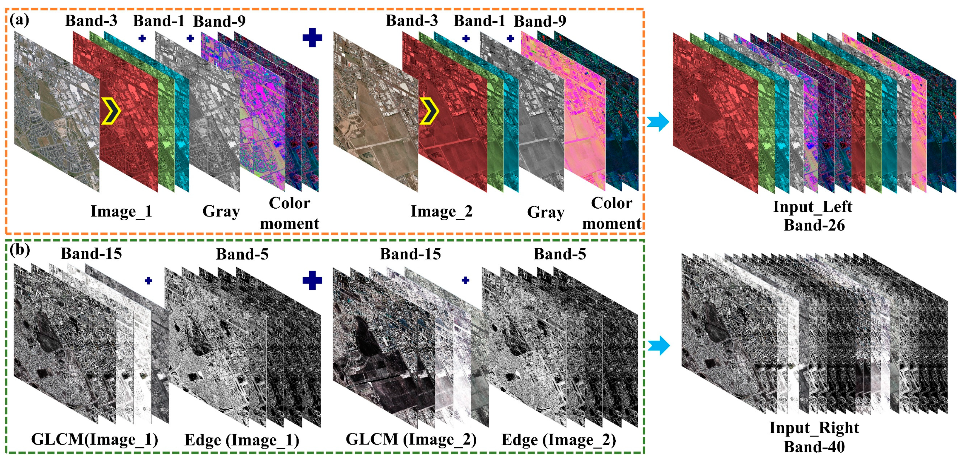A variety of features derived from remote sensing data tend to show characteristics such as stable nature, little impact by radiation differences, and not easily affected by remote sensing image time phase changes [3]. Using spatial or spectral features to detect changes in the state of objects or regions has become a hot spot for researchers. In addition, the phenomenon of “the same object with the different spectrum, the same spectrum of different matter” appears in large numbers in HR/VHR remote sensing images, making it more difficult to detect small and complex objects such as buildings or roads in cities. Emerging deep learning methods have the potential to extract features of individual buildings in complex scenes. However, the feature extraction method of deep learning represented by convolution operation only extracts the abstract features of the original image through the continuous deepening of the number of convolution layers and do not consider the use of useful derivative features of the ground objects [3,27]. Various feature information derived from the original image, such as color, texture, shape, et al., can also be used as input to the network to participate in the process of information mining and abstraction. As far as we know, many existing networks fail to take multiple features as input to participate in task execution.

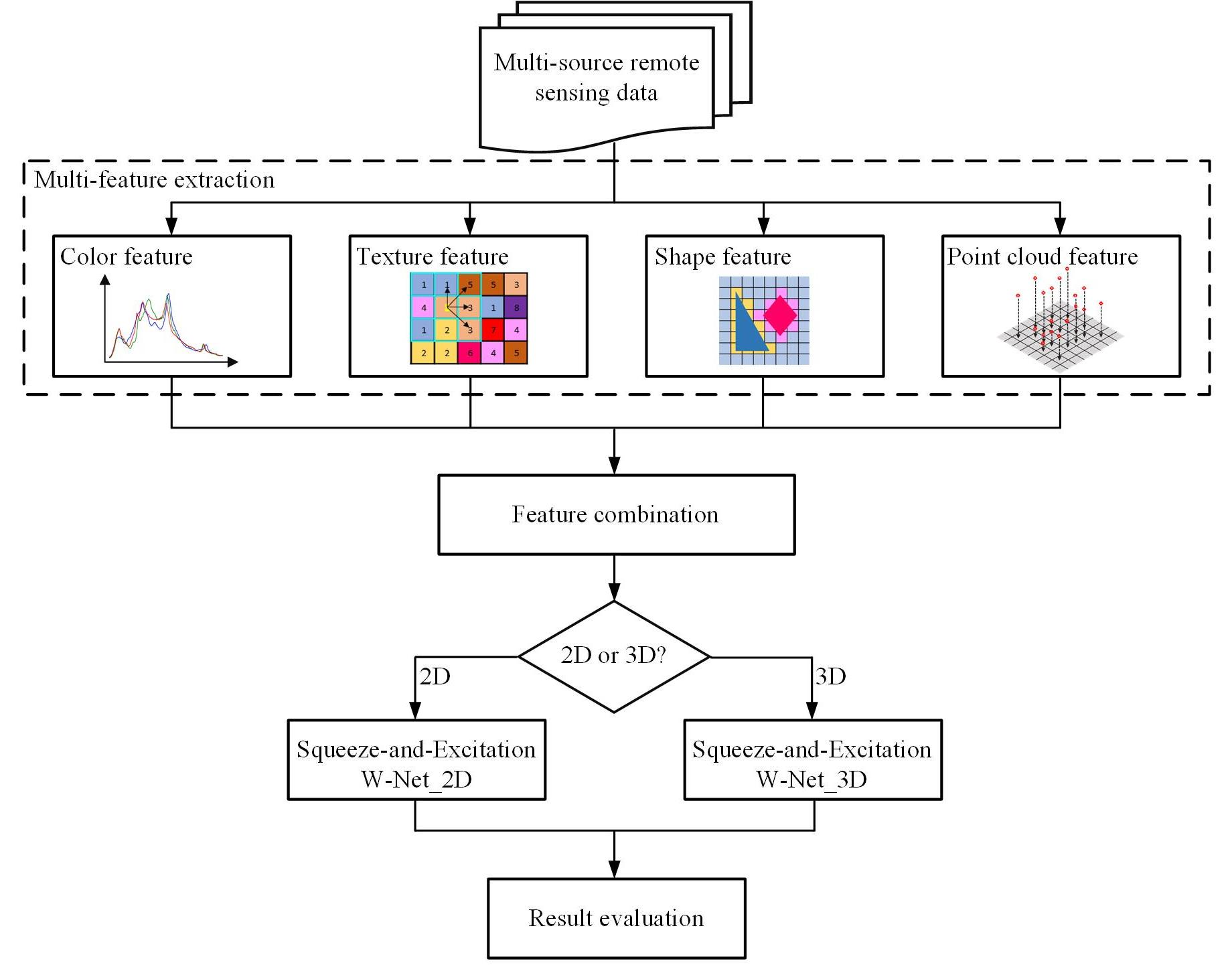
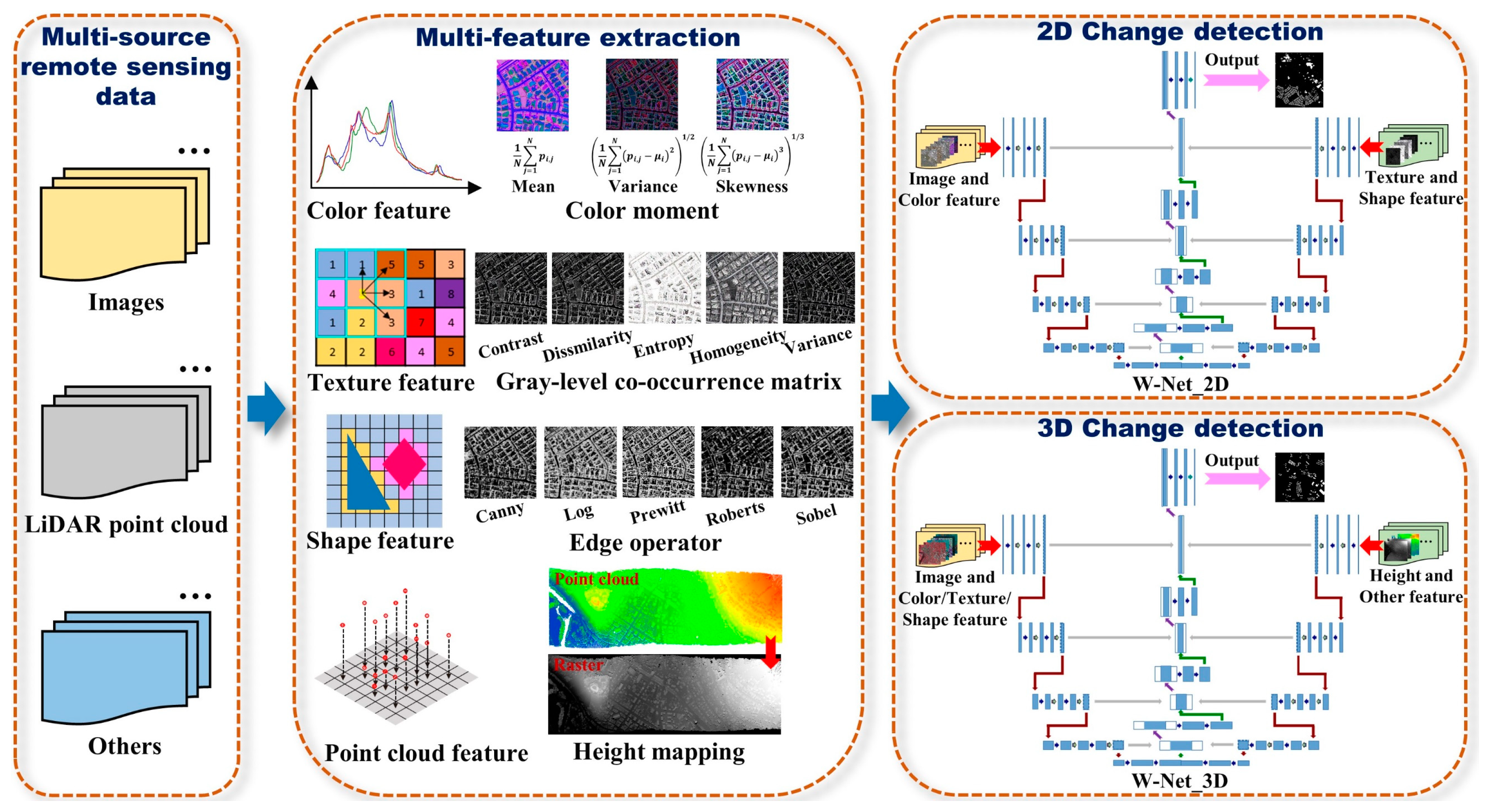
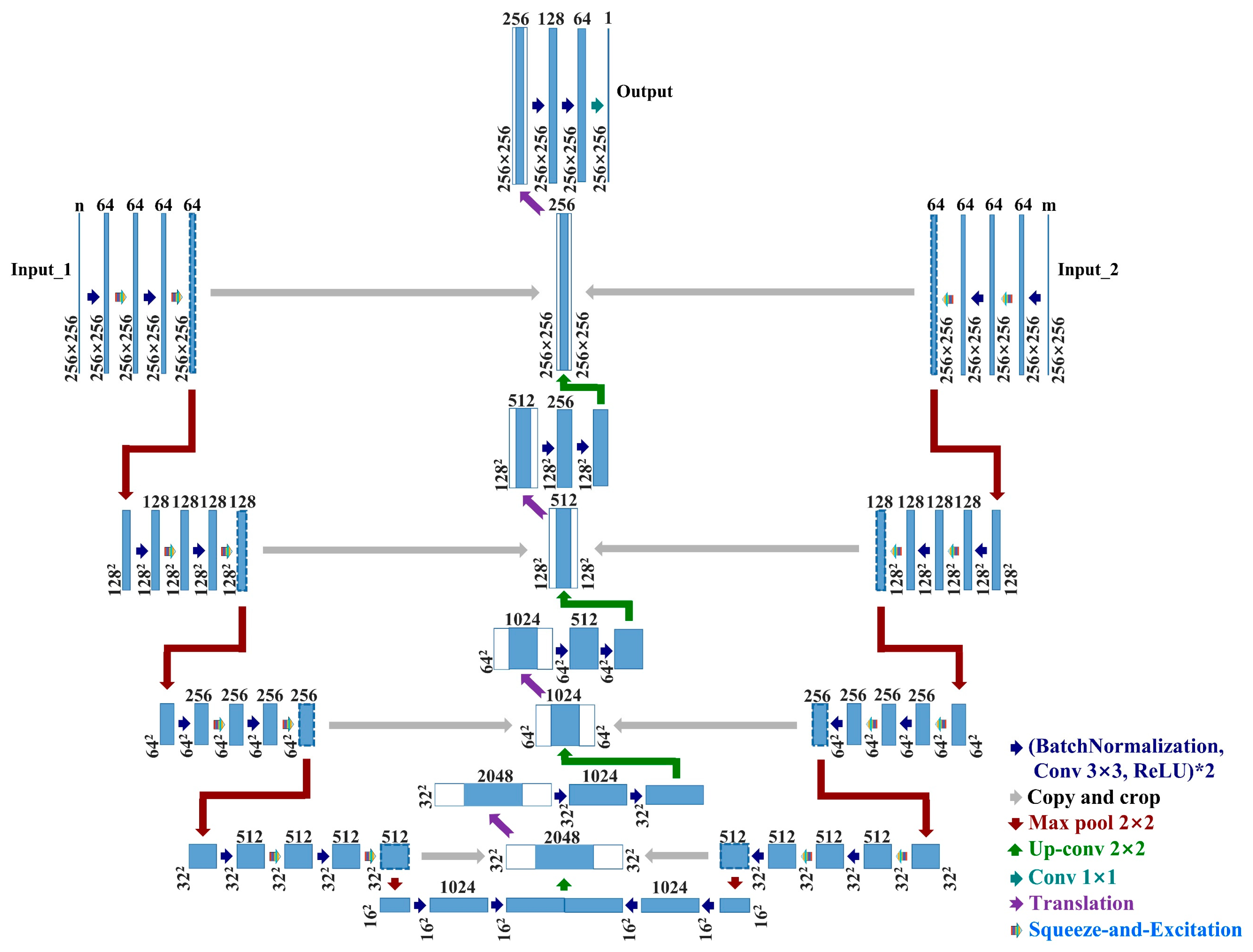
In this article, based on U-Net, we designed a new type of bilateral end-to-end W network. It can simultaneously input multi-source/multi-feature homogeneous and heterogeneous data and consider the internal relationship of input data through the squeeze-and-excitation strategy. We named it squeeze-and-excitation W-Net. Although there have been related studies on network transformation based on U-Net [50,51], as far as we know, we are the first to transform U-Net into a more valuable network. It has two-sided input and single-output, independent weights on both sides can take into account the data on both sides (homogeneous and heterogeneous data) and can be used for change detection tasks in the field of remote sensing. The main contributions of this article are concluded as follows:

(1)

The proposed squeeze-and-excitation W-Net is a powerful and universal network structure, which can learn the abstract features contained in homogeneous and heterogeneous data through a structured symmetric system.

(2)

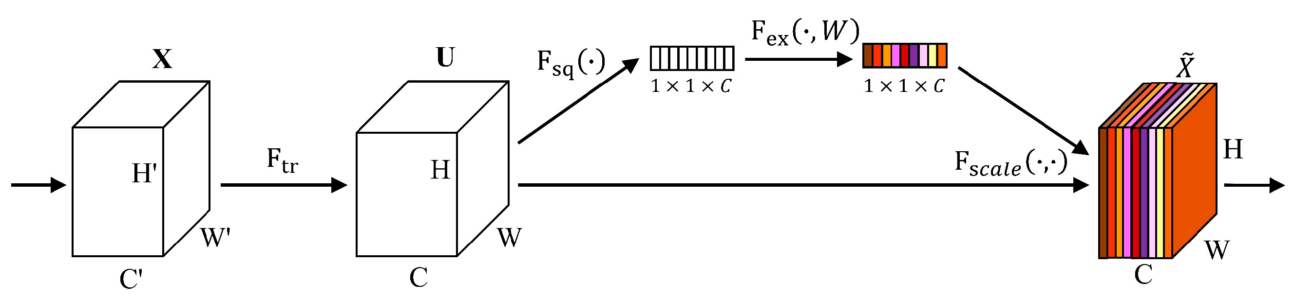
The form of two-sided input not only satisfies the input of multi-source data but also is suitable for multiple features derived from multi-source data. We innovatively introduced the squeeze-and-excitation module as a strategy for explicit modeling of the interdependence between channels, which makes the network more directional and can recalibrate the feature channels, emphasize essential features, and suppress secondary features. Moreover, the squeeze-and-excitation module is embedded between each convolution operation, which can overcome the insufficiency of the convolution operation that can only take into account the features information in the local receptive field and improve the global reception ability of the network.

(3)

The idea of multi-source and multi-feature combination as model input integrates information advantages such as spectrum, texture, and structure, which can significantly improve the robustness of the model. For buildings, which present complex spatial patterns, have multi-scale features, and have large differences between individuals, they are more targeted, and the detection accuracy of the model is significantly higher.

The rest of the article is organized as follows. The second section introduces in detail the construction process of squeeze-and-excitation W-Net, the production details of multi-feature input, and the evaluation method of the network. The third section is the data set information, network settings, experiments, and results. The fourth section is the discussion part. And the fifth section summarizes the article.

2. Methodology

The proposed 2D and 3D change detection method for buildings based on squeeze-and-excitation W-Net includes three parts: (1) Construct the squeeze-and-excitation W-Net to satisfy the input of homogeneous data, heterogeneous data, and multi-feature combined images. When performing 2D change detection, the left and right sides of the network, accept the original image and the characteristic image, respectively. When performing 3D change detection, the left and right sides of the network accept the original image and its feature image and height data and its feature image, respectively. (2) Use color moment, gray level co-occurrence matrix (GLCM), and edge operator to extract the color feature, texture feature, and shape feature of the image, respectively, and merge the extracted features with the original image as network input. (3) Train the squeeze-and-excitation W-Net, save the model with higher validation accuracy and lower validation loss, and perform change detection in the experimental area. The workflow of the proposed change detection method is shown in Figure 1.

2.1. The Proposed Novel Squeeze-and-Excitation W-Net

2.1.1. Bilaterally Symmetrical End-to-End Network Architecture

Although the convolutional layer of CNN is a structure suitable for extracting spatial context features and spectral features simultaneously, its receptive field is limited, and the output is a category label corresponding to a fixed-size image. It cannot achieve the pixel-level positioning of category labels in visual tasks [45]. However, the image processing form of semantic segmentation can classify each pixel on the image to obtain the image classification result of the located pixel.

U-Net is an extension of FCN and is currently a widely used semantic segmentation network with good scalability [52]. The excellent characteristics of U-Net make it widely used in remote sensing image classification and change detection and have achieved good results [50,52]. However, the number of convolutional layers is small, and the Batch Normalization layer is lacking, which causes problems such as low learning efficiency, learning effect greatly affected by the initial data distribution, and gradient explosion in the backpropagation process [3,47,52]. In addition, the U-Net single-side input and single-side output network structure also limits the comprehensive use of multi-source remote sensing data, making the data input single, and the feature extraction of the data limited to a small number of convolution operations. Although its skip connection strategy can merge low-dimensional features and high-dimensional features, it is challenging to balance the effective extraction of features and the comprehensive use of data in the face of complex data types and diversified data features.

In order to make up for these shortcomings of U-Net, we designed a two-sided input W-shaped network, which contains a contracting path on both sides and an expansive path in the middle. The contraction path on both sides contains four sets of encoding modules, but the encoding module deepens the number of layers of convolution and introduces the Batch Normalization layer. The expansion path contains four sets of decoding modules and also adds the Batch Normalization layer. Among them, the Batch Normalization layer can normalize the input data of each batch with the mean and variance so that the input of each layer maintains the same distribution, which can speed up the speed of model training. In addition, the Batch Normalization layer can increase noise through the idea of updating the mean and variance of each layer, thereby increasing the robustness of the model and effectively reducing overfitting. The calculation of the Batch Normalization layer is performed as in Equation (1)

$${\widehat{x}}^{\left(k\right)}=\frac{x^{\left(k\right)}-E\left[x^{\left(k\right)}\right]}{\sqrt{Var\left[x^{\left(k\right)}\right]}}$$

(1)

where, ${\widehat{x}}^{\left(k\right)}$ is the activation value of the $k$-th neuron after transformation; $x^{\left(k\right)}$ is the neuron of each batch of training data; $E\left[x^{\left(k\right)}\right]$ is the average value of each batch of training data neurons; $\sqrt{Var\left[x^{\left(k\right)}\right]}$ is the standard deviation of the activation of each batch of training data neurons.

In addition, in order to meet the needs of change detection tasks, we use a binary cross-entropy function as the loss function of the W-shaped network in the network. The formula is performed as in Equation (2)

$$Loss=-\frac{1}{N}{\displaystyle \sum }_{n=1}^N{y}_n·log\left({\widehat{y}}_n\right)+\left(1-{\widehat{y}}_n\right)·log\left(1-{\widehat{y}}_n\right)$$

(2)

where, $N$ represents the number of predicted values output by the model; $y_n$ is the sample label; ${\widehat{y}}_n$ is the predicted label of the sample by the model; the optimizer used by the network is Adam.

The skip connection strategy of the W-shaped network is extended to two sides. That is, the low-dimensional features of symmetrical positions on both sides are copied to the expansive path, combined with the high-dimensional features, and convolution is performed. This strategy can divide different data sources into two inputs, avoid the mutual exclusion of data, better retain the original characteristics of the data, and give play to the most significant advantage between different data. In addition, the network weights of the contracting paths on both sides are independent of each other. During the back propagation of the network, the loss values obtained from the loss function are transmitted to both sides at the lowest end of the contracting path, and the network weights on both sides are updated at the same time. In this way, it can achieve the purpose of non-linear simulation of multi-source data at the same time.

2.1.2. Squeeze-and-Excitation W-Net

The W-shaped network is improved on the basis of U-Net, expanding the path of data input, deepening the convolution operation, accelerating the training speed of the model, improving the robustness of the model, and effectively preventing overfitting. However, the convolution operation can only be along the data input channel, fusing the spatial and channel information in the local receptive field [53]. In addition, when comprehensively considering the multi-source data and the multiple features derived from it, it is difficult to model the spatial dependence of the data based on the information feature construction method of the local receptive field. Moreover, the repeated convolution operation without considering the spatial attention is not conducive to the extraction of useful features.

We introduced the attention mechanism [54,55,56] strategy, using global information to explicitly model the dynamic non-linear relationship between channels, which can simplify the learning process and enhance the network representation ability. The main function of the attention mechanism is to assign weights to each channel to enhance important information and suppress secondary information. The main operation can be divided into three parts: squeeze operation $F_{sq}\left(·\right)$, excitation operation $F_{ex}\left(·,W\right)$, and fusion operation $F_{scale}\left(·,·\right)$. Its operation flow chart is shown in Figure 2.

The squeeze operation uses a global average pooling method to compress features along the spatial dimension and scale each two-dimensional feature map to a real number, which has a global receptive field and can represent global information. When the input is $X\in R^{H^{\prime }\times W^{\prime }\times C^{\prime }}$, the output after the regular convolution operation is $U\in R^{H\times W\times C}$. The squeeze operation is based on $U$, and the input of size $H\times W\times C$ can be compressed into $1\times 1\times C$ feature description. For a particular feature map, the squeeze calculation is performed as in Equation (3)

$$z_c=F_{sq}\left(u_c\right)=\frac{1}{H\times W}{\displaystyle \sum }_{i=1}^H{\displaystyle \sum }_{j=1}^W{u}_c\left(i,j\right)$$

(3)

where, $u_c$ is the c-th feature map; $i,j$ represent the pixel positions in the feature map.

The squeeze operation only obtains a 1 × 1 global descriptor, which cannot be used as the weight of each feature map. However, the excitation operation using two fully connected layers and the Sigmoid function can more comprehensively capture the interdependence between channels. Its calculation formula is performed as in Equation (4)

$$s=F_{ex}\left(z,W\right)=\sigma \left(g\left(z,W\right)\right)=\sigma \left(W_2\delta \left(W_{1}z\right)\right)$$

(4)

where, $z$ is global description; $\delta$ is the ReLu activation function; $W_1$,$W_2$ represents the weight matrix of two fully connected layers; $\sigma$ represents the Sigmoid function.

The last step is the fusion operation. That is, the channel weight calculated by the excitation operation is fused with the original feature map, and the calculation is as shown in Equation (5)

$${\stackrel{\sim }{x}}_c=F_{scale}(u_c,s_c)=s_c*u_c$$

(5)

where, $s_c$ is the c-th global description; $u_c$ is the c-th original feature map.

We innovatively embed the squeeze-and-excitation module into the left and right contracting paths of the W-shaped network and add a squeeze-excitation layer after each convolution to learn the dependency of feature channels to improve the learning ability of the network. This can better deal with the complexity of multi-source and multi-feature data, and obtain a network that is more robust and more sensitive to specific features. The structure of squeeze-and-excitation W-Net is shown in Figure 3.

2.2. Multi-Feature Mapping and Information Mining

In this article, we are in order to provide more detailed and comprehensive, reliable data for the network. In terms of color, texture, and shape, a variety of features are extracted from the original image, and these features are combined with the original image as the input of the network.

2.2.1. Color Moment for Color Features Extraction

The color feature is the most widely used visual feature in color images, and it is widely used in image retrieval and video retrieval [57]. In addition, it has a small dependence on the size, direction, and angle of the image, stable performance, and strong robustness to image degradation and resolution changes [58]. Since the color information in the image is mostly distributed in the low-order moments of the image, we extract the color features of the image by calculating the first-order moment (mean), second-order moment (variance), and third-order moment (skewness) of the image. The color feature map of the entire image is extracted with a fixed-size sliding window. The calculation equations are shown in Equations (6)–(8)

$$Mean={\mu }_k=\frac{1}{N}{\displaystyle \sum }_{\left(i,j\right)=1}^N{p}_{i,j}^k$$

(6)

$$Variance={\sigma }_k={\left(\frac{1}{N}{\displaystyle \sum }_{\left(i,j\right)=1}^N{\left(p_{i,j}^k-{\mu }_k\right)}^2\right)}^{1/2}$$

(7)

$$Skewness=s_k={\left(\frac{1}{N}{\displaystyle \sum }_{\left(i,j\right)=1}^N{\left(p_{i,j}^k-{\mu }_k\right)}^3\right)}^{1/3}$$

(8)

where, $p_{i,j}^k$ is the k-th color component of the (i,j)-th pixel in the image; N is the number of pixels in the image.

2.2.2. GLCM for Texture Features Extraction

The texture feature is a visual feature that reflects the homogeneity phenomenon in the image, and it can reflect the periodically changing structural organization and arrangement properties of the surface of the ground object [59]. It can be obtained according to the change rule of the gray value of the image pixel within a specific range and is used to analyze better and understand the original image. The local texture feature is represented by the gray distribution of the pixel and its neighborhood, and the global texture feature is the repetition of local features. Therefore, there is a certain gray-scale relationship between two non-adjacent pixels in the image, that is, gray-scale spatial correlation characteristics. Capturing and quantitatively describing this spatial correlation characteristic helps to analyze the original image from the texture level. GLCM can quantitatively describe the texture characteristics of the image with the gray-scale spatial correlation characteristics in the image [59,60]. GLCM mainly extracts texture through the conditional probability density between gray levels of the image, which is a unique matrix. It describes a specific relationship between the gray values of adjacent pixels or adjacent pixels whose distance is a specific value. Usually, some scalars are used to characterize GLCM. In this paper, five scalars, including variance, homogeneity, contrast, dissimilarity, and entropy, were used to describe image texture characteristics. The equations used are shown in Equations (9)–(13)

$$GLC{M}_{Variance}={\displaystyle \sum }_i{\displaystyle \sum }_{j}p\left(i,j\right){\left(i-\mu \right)}^2$$

(9)

$$GLC{M}_{Homogeneity}={\displaystyle \sum }_i{\displaystyle \sum }_j\frac{p\left(i,j\right)}{1+{\left(i-j\right)}^2}$$

(10)

$$GLC{M}_{Contrast}={\displaystyle \sum }_i{\displaystyle \sum }_j{\left(i-j\right)}^2{p}^2\left(i,j\right)$$

(11)

$$GLC{M}_{Dissimilarity}={\displaystyle \sum }_i{\displaystyle \sum }_j\left(i-j\right)p\left(i,j\right)$$

(12)

$$GLC{M}_{Entropy}=-{\displaystyle \sum }_i{\displaystyle \sum }_{j}p\left(i,j\right)lo{g}_{2}p\left(i,j\right)$$

(13)

where,$p\left(i,j\right)=p\left(i,j,\delta ,\theta \right)=\left\{\left(x,y\right),\left(x+dx,y+dy\right)ϵN\times N|f\left(x,y\right)=i,f\left(x+dx,y+dy\right)=j\right\}$; $\left(x,y\right)$ is the reference pixel; $\left(x+dx,y+dy\right)$ is the shifting pixel; $f\left(x,y\right)=i$ represents that the gray value of the reference point is $i$; $f\left(x+dx,y+dy\right)=j$ represents the gray value of the shifting pixel is $j$; the step is fixed at a certain angle, $\delta$ is the shifting step size, and $\theta$ is the shifting angle.

2.2.3. Edge Detection Operator for Shape Features Extraction

Shape features are important information describing target objects, and they play an important role in the identification and detection of target objects [58]. It can provide clear edge information of objects and retain important structural attributes in the image. When detecting small and complex objects such as buildings, it can make up for the deficiencies of the spectrum and texture features that are easily confused and difficult to detect. In this paper, five edge detection operators, Canny, Log, Prewitt, Roberts, and Sobel, were used to extract the shape features of the objects in the image.

2.2.4. Combine Multiple Features

There are considerable differences between buildings, and conventional remote sensing methods are difficult to comprehensively describe their spectrum, texture, shape, and other features [61,62]. We extracted the color, texture, and shape features contained in the original data and combined the original data with these derived features to form an “artificial high-dimensional image” that contained rich image information. “Artificial high-dimensional image” was used as the input of the squeeze-and-excitation W-Net network, that is, using the means of deep learning to perform abstract learning and deep feature extraction of the original remote sensing data and features to achieve a detailed, comprehensive, and accurate description of the object to be detected.

The form of feature combination adopts staggered arrangement and grouping. Taking a 2D experiment as an example, the input on the left of the network is a combination of the original image, grayscale image, and color features, and the input on the right is a combination of texture features and shape features. The number of bands (Band-number) corresponding to each is shown in

Table 1. The number of bands for each feature.

Date	Image	Gray	Color_moment	GLCM	Edge
Band number	3 × 2	1 × 2	9 × 2	3 × 5 × 2	1 × 5 × 2

, and the combination is shown in Figure 4.

2.3. Accuracy Assessment

To validate the effectiveness of the proposed squeeze-and-excitation W-Net. This paper evaluated it from two perspectives: (1) calculate the overall accuracy (OA), F_1 value, missing alarm (MA), and false alarm (FA) based on reference data to evaluate the network’s ability to detect buildings; (2) compared with some widely used change detection methods, including RCVA, support vector machine (SVM), random forest (RF), deep belief network (DBN), U-Net, SegNet, and DeepLabv3+.

2.3.1. Comparison with Ground Truth Data

The overall accuracy represents the ratio of the number of pixels correctly recognized by the model to the number of all samples, and it represents the ability of the model to classify positive or negative samples correctly. The calculation is as in Equation (14)

$$OA=\frac{TP+TN}{TP+FP+TN+FN}$$

(14)

where, TP is the number of positive samples classified by the model correctly; FN is the number of positive samples classified by the model incorrectly; TN is the number of negative samples classified by the model correctly; FP is the number of negative samples classified by the model incorrectly.

The $F_1$ value is a comprehensive index that reflects precision and recall. The precision is the proportion of correctly classified positive samples in all positive samples classified, and the recall is the proportion of correctly classified positive samples in all positive samples. For calculation, Equations (15) and (16) are used:

$$Precision=\frac{TP}{TP+FP},Recall=\frac{TP}{TP+FN}$$

(15)

$$F_1=\frac{2*Precision*Recall}{Precision+Recall}$$

(16)

The missing alarm is the proportion of positive samples that are mistakenly classified as negative samples to all positive samples, and the false alarm is the proportion of negative samples that are mistakenly classified as positive samples to all negative samples. They reflect the degree of misjudgment of the sample by the model. For calculation the Equations (17) and (18) are used:

$$MA=\frac{FN}{TP+FN}$$

(17)

$$FA=\frac{FP}{TN+FP}$$

(18)

2.3.2. Comparison with Other Methods

We adopted seven widely used change detection methods and classified them into traditional methods (RCVA), machine learning methods (SVM and RF), transition methods (DBN) from machine learning to deep learning (hereinafter referred to as transition methods), and deep learning methods (U-Net, SegNet, and DeepLabv3+). We evaluated the performance of squeeze-and-excitation W-Net from these four aspects. Compared with traditional methods, machine learning methods, and transition methods, the evaluation index was mainly used as a reference basis. Compared with the deep learning method, in addition to the evaluation index, the model was evaluated in terms of running time and convergence rate. The description of each method is as follows:

(1)

RCVA [17] is an effective unsupervised multispectral image change detection method. Based on the RCVA principle, this paper traverses all the pixels of the two images to obtain the changing area.

(2)

SVM [63] is a machine learning algorithm based on the small sample statistics theory. It aims to find the optimal decision hyperplane to separate the sample data when the data points cannot be separated linearly. We used manually selected sample points to extract training feature values and train the SVM classifier.

(3)

RF [64] is a machine learning algorithm that combines ensemble learning theory and the random subspace method. Since it uses the bootstrap resampling technique to select training samples, we only provided training data and labels for RF.

(4)

DBN [65,66] is developed from the biological neural networks and shallow neural networks. It is a probabilistic generative model, which is composed of multi-layer restricted Boltzmann machine (RBM) and BP network. It uses the joint probability distribution to infer the sample data distribution. In this paper, a vector of gray values of pixels arranged in a fixed window is used as input to train multi-layer RBM, and a small number of labels are used to optimize the model.

(5)

U-Net is a classic semantic segmentation network, developed from FCN. We used the most primitive U-Net model for image segmentation experiments.

(6)

SegNet [67] is a semantic segmentation network based on deep convolution and fusion encoding-decoding structure. This article used the original network architecture developed from FCN and VGG16.

(7)

DeepLabv3+ [68] is considered one of the most advanced algorithms for semantic segmentation. It uses the encoding-decoding structure for multi-scale information fusion while retaining the original dilated convolution and ASSP layer. Its backbone network uses the Xception model, which improves the robustness and operating rate of semantic segmentation.

3. Experiments

To validate the effectiveness of the proposed method, we conducted 2D and 3D BCD experiments, respectively, and both experiments contain two sets of sub-experiments. The original remote sensing data for 2D experiments are VHR remote sensing images, and the 3D experiments were VHR remote sensing images and airborne LiDAR point cloud data.

3.1. Datasets

3.1.1. Datasets for 2D Experiments

The data for the first set of sub-experiments came from the Building change detection dataset of the WHU Building Dataset [69]. The data are aerial images, acquired in April 2011 and April 2016, with a resolution of 0.075 m, including red, green, and blue bands. In the area covered by the image, a magnitude 6.3 earthquake occurred in February 2011, and the buildings were seriously damaged. When the image of the area was reacquired in 2016, the number of buildings increased significantly, and the types and shapes of the buildings were rich, so It is a high-quality data set for BCD. In this experiment, an area (red rectangle) with a size of 11,654 × 10,065 pixels and more building changes was selected from the data set as the experimental area. The image of the experimental area and the reference change map are shown in Figure 5. Among them, the reference change map is provided by the data publisher.

The data of the second group of sub-experiments was the Multi-temporal Scene WuHan (MtS-WH) Dataset, which includes two large-size 7200 × 6000 HR remote sensing images obtained by IKONOS sensors, covering the area of Wuhan, China Hanyang District. The images were obtained in February 2002 and June 2009, respectively, and fused by the GS algorithm, with a resolution of 1 m and four bands (blue, green, red, and near-infrared). Since the MtS-WH data set is mainly used for theoretical research and validation of scene change detection methods, and the original data only provides the category label of the scene, to obtain the changing scene, we obtained the reference change map of the building area by comparing the scene categories. The image and label are shown in Figure 6.

3.1.2. Datasets for 3D Experiment

The data of the first set of 3D sub-experiments was the Vaihingen data set provided by ISPRS-Commision II Working Group II/4. The data set was obtained by the German Association of Photogrammetry and Remote Sensing in the Vaihingen area of Stuttgart, Germany. In addition to VHR remote sensing images (near-infrared, red, green) and reference data, DSM and LiDAR data are also provided. The spatial resolution of the VHR remote sensing image and DSM was 0.09 m. LiDAR data was acquired by an ALS50 sensor on 21 August 2008.

Since the Vaihingen data set contains only one period of data, we selected a certain number of buildings as the assumed change area in order to verify the effectiveness of the method in this paper. In addition, we used the CSF Plugin Instruction [70] tool to isolate the ground points in the LiDAR point cloud, generated a DEM based on the point cloud data, and resampled it to a spatial resolution of 0.09 m. We used the difference between DSM and DEM to obtain the nDSM data model that eliminated the influence of terrain and records the height information of all ground objects relative to the ground. The Vaihingen data set, simulation data, and reference data are shown in Figure 7.

The data of the second set of 3D sub-experiments were historical Google Earth images and UAV LiDAR point cloud data we independently obtained. The data covers an area in Changchun City, Jilin Province, China, with an image resolution of 0.13 m and a size of 4332 × 5267 pixels. The two phases of HR images were obtained in May 2009 and May 2019, including three bands of red, green, and blue. UAV LiDAR point cloud data were obtained in May 2019. Due to the lack of point cloud data corresponding to May 2009, we still assumed the point cloud data of 2009 by means of simulation. HR remote sensing image, point cloud, and its simulation data, reference data are shown in Figure 8.

3.2. Network Training and Change Detection

3.2.1. Network Training and Parameter Selection

We constructed the squeeze-and-excitation W-Net based on the TensorFlow framework. For the operating environment we used an Intel(R) Core(TM) i9-990KF CPU, and a NVIDIA GeForce RTX 2080 SUPER GPU (8 GB). In the four sub-experiments, the input image size at the left and right ends of the network was 128 × 128 pixels, and the amount of training data in each batch was 16. In order to facilitate comparison with other methods and minimize the time expenditure, the epoch of each experiment was set to 100, the training images used in the experiment were 1000, and the reduction ratio set in the network was 16, as provided in the original article [53].

For the traditional method, we obtained the binary change map by setting the threshold. For the machine learning method, we used the manually selected sample points to train the classifier to get the detection result. For the transition method, we used the reference change map to select the appropriate number of samples to train the network to get the detection results. For the deep learning method, we choose 1000 training images, set the epoch to 100, used the recommended hyperparameters, and trained the network to get the detection results.

3.2.2. 2D Change Detection

The original data in 2D experiments (experiment 1 and experiment 2) only contained remote sensing images. The input of the first, second, and third methods was the original remote sensing image. The input of the fourth method is the original image and the feature image. The experimental details of each method are shown in

Table 2. Details of experiment 1.

Classes	Methods	Details	Time
Traditional	RCVA	Window size: 3 × 3, Threshold: 100	213.28 min
Machine-learning	SVM	Number of sample points: building 233, others 266	99.54 min
	RF	Number of trees: 108, Maximum depth of the tree: 8	15.69 min
Transitional	DBN	Window size: 2 × 2, Number of samples: 5000	9.44 min
Deep-learning	U-Net	Minimum loss: 0.62, Maximum accuracy: 97.44%	16.38 min
	SegNet	Minimum loss: 0.11, Maximum accuracy: 96.30%	36.35 min
	DeepLabv3+	Minimum loss: 0.12, Maximum accuracy: 96.76%	9.34 min
	Proposed	Minimum loss: 0.27, Maximum accuracy: 97.68%	34.06 min

RCVA: robust change vector analysis; SVM: support vector machine; RF: random forest; DBN: deep belief network.

and

Table 3. Details of experiment 2.

Classes	Methods	Details	Time
Traditional	RCVA	Window size: 3 × 3, Threshold: 80	76.22 min
Machine-learning	SVM	Number of sample points: building 200, others 230	241.91 min
	RF	Number of trees: 108, Maximum depth of the tree: 8	4.32 min
Transitional	DBN	Window size: 2 × 2, Number of samples: 5000	5.32 min
Deep-learning	U-Net	Minimum loss: 0.56, Maximum accuracy: 78.18%	25.48 min
	SegNet	Minimum loss: 0.51, Maximum accuracy: 81.55%	35.59 min
	DeepLabv3+	Minimum loss: 0.42, Maximum accuracy: 83.42%	3.58 min
	Proposed	Minimum loss: 0.24, Maximum accuracy: 83.76%	33.05 min

, and the detection results are shown in Figure 9 and Figure 10.

3.2.3. 3D Change Detection

3D change detection also included two sets of sub-experiments (experiment 3 and experiment 4). Although DSM data was added to the 3D experiment, the image of the first group of sub-experiment was simulated data, so the comparative experiments of the first, second, and third methods were not performed. The experimental details of each method are shown in

Table 4. Details of experiment 3.

Classes	Methods	Details	Time
Deep-learning	U-Net	Minimum loss: 0.30, Maximum accuracy: 99.50%	34.72 min
	SegNet	Minimum loss: 0.04, Maximum accuracy: 99.02%	36.62 min
	DeepLabv3+	Minimum loss: 0.02, Maximum accuracy: 99.57%	15.01 min
	Proposed	Minimum loss: 0.06, Maximum accuracy: 99.26%	34.42 min

and

Table 5. Details of experiment 4.

Classes	Methods	Details	Time
Traditional	RCVA	Window size: 3 × 3, Threshold: 120	35.15 min
Machine-learning	SVM	Number of sample points: building 558, others 1360	335.07 min
	RF	Number of trees: 108, Maximum depth of the tree: 8	2.05 min
Transitional	DBN	Window size: 2 × 2, Number of samples: 5000	9.68 min
Deep-learning	U-Net	Minimum loss: 0.19, Maximum accuracy: 99.61%	33.81 min
	SegNet	Minimum loss: 0.03, Maximum accuracy: 99.02%	37.46 min
	DeepLabv3+	Minimum loss: 0.07, Maximum accuracy: 99.19%	1.45 min
	Proposed	Minimum loss: 0.009, Maximum accuracy: 99.40%	34.40 min

, and the detection results are shown in Figure 11 and Figure 12.

According to the formula in Section 2.3.1, the evaluation index corresponding to the four groups of detect results were calculated, as shown in

Table 6. Accuracy assessment on 2D change detection results.

Methods	Experiment 1				Experiment 2
	OA	F1	MA	FA	OA	F1	MA	FA
RCVA	0.8097	0.2821	0.6211	0.1431	0.6233	0.3087	0.7916	0.0958
SVM	0.8411	0.4860	0.2385	0.1502	0.7008	0.6215	0.3915	0.2366
RF	0.7093	0.3624	0.1628	0.3047	0.6590	0.5698	0.4405	0.2736
DBN	0.9020	0.6539	0.0620	0.1019	0.7210	0.6953	0.2114	0.3247
U-Net	0.9646	0.8014	0.2771	0.0089	0.7742	0.7387	0.2091	0.2372
SegNet	0.9578	0.7985	0.1520	0.0302	0.7669	0.6597	0.4403	0.0928
DeepLabv3+	0.9546	0.7654	0.2494	0.0231	0.7682	0.7359	0.1998	0.2534
Proposed	0.9722	0.8569	0.1564	0.0137	0.7699	0.7409	0.1849	0.2608

OA: overall accuracy; F1: F1 value; MA: missing alarm; FA: false alarm.

and

Table 7. Accuracy assessment on 3D change detection results.

Methods	Experiment 1				Experiment 2
	OA	F1	MA	FA	OA	F1	MA	FA
RCVA	/	/	/	/	0.7647	0.2442	0.6271	0.1908
SVM	/	/	/	/	0.8865	0.5164	0.4059	0.0803
RF	/	/	/	/	0.8953	0.5438	0.3878	0.0726
DBN	/	/	/	/	0.8940	0.6387	0.0815	0.1087
U-Net	0.9940	0.9523	0.0609	0.0023	0.9956	0.9784	0.0278	0.0017
SegNet	0.9901	0.9208	0.0919	0.0044	0.9906	0.9552	0.0183	0.0084
DeepLabv3+	0.9896	0.9138	0.1370	0.0018	0.9916	0.9585	0.0481	0.0039
Proposed	0.9946	0.9571	0.0532	0.0022	0.9956	0.9784	0.0288	0.0016

.

It can be seen from Table 6 and Table 7 that, except for individual cases, the detection results obtained by the proposed method, OA and F1 were both the maximum, and MA and FA are both the minimum. Moreover, except for the generally low detection accuracy of experiment 2, the OA values of the proposed methods were all greater than 0.97, and the F1 values were all greater than 0.86. This shows that the squeeze-and-excitation W-Net proposed in this paper with multi-source and multi-feature data as input could obtain higher quality detection results than other methods. Furthermore, our proposed network not only surpassed traditional methods, machine learning methods, and transition methods but also performed better than the typical semantic segmentation network of deep learning methods. It can also be seen Figure 9, Figure 10, Figure 11 and Figure 12 that the detection results obtained by the method in this paper could accurately and clearly reflect the changing buildings. This proves that the squeeze-and-excitation W-Net we designed can be successfully applied to the 2D and 3D change detection of buildings.

4. Discussion

To evaluate the proposed method fully. Section 4.1 provides an intuitive evaluation of the methods from the aspect of comparison methods. Section 4.2 analyzes the performance of the squeeze-and-excitation network. The influence of multi-feature input on the model is discussed in Section 4.3.

4.1. Comparison with Previous Studies

The seven previous research methods used in this article were all representative and could fully illustrate the advantages of our method. RCVA eliminates the influence of image registration errors by considering neighborhood information [17]. It divides the spectral change intensity value of the pixel by the threshold and then obtains the changing area, which limits the detection accuracy to the quality of the threshold selection. However, the linear threshold does not have much physical meaning and is highly subjective. Besides, the degree of confusion of pixel spectral values in HR remote sensing images is so great that RCVA, which simply takes pixel spectral values as the research object, appears powerless when processing HR remote sensing images. SVM generates the optimal classification hyperplane by solving a convex quadratic programming problem [63]. It can perform non-linear classification tasks. However, the training of the classifier requires enough training samples. We manually select a limited amount of training samples, and the detection results obtained after training the SVM are not ideal. The indexes in Table 6 and Table 7 also show that the hand-selected training sample points of experiment 4 are several times more than experiment 1 and experiment 2. Compared with experiment 1, the OA and F1 of experiment 4 were increased by more than 5% and 3%, respectively, and the FA value was reduced by more than 7%. This shows that the number of training sample points directly affects the detection performance of SVM. Similarly, this situation is the same for RF. Because compared with experiment 1, the OA and F1 of experiment 4 were increased by more than 18%, and the FA was reduced by more than 23%. However, hyperparameters such as the number of decision trees and the maximum depth of the decision tree would affect the classification effect of RF [64]. However, under the premise of a fixed number of samples, we found that by adjusting the hyperparameters, the influence of the hyperparameters is much smaller than the training samples. It can also be observed Figure 9, Figure 10, Figure 11 and Figure 12 that although the detection results of SVM and RF have a certain degree of error, they can reflect the main change areas of the building. This shows that compared to traditional methods, machine learning methods have certain advantages. The DBN network belonging to the transition method has higher OA and F1 and relatively lower MA and FA. However, the price of this improvement is the need to feed a larger number of training samples. We automatically selected 5000 training samples by reference map, avoiding the time-consuming way of manually selecting samples. This method of automatically selecting training samples can provide sufficient training samples for DBN. The trained model has a better detection effect, which may be related to this.

On the whole, the detection results of deep learning methods are of higher quality than the other three types of methods. Figure 9 and Figure 12e–h show that the building areas were relatively straightforward and accurate, and there was almost no large-scale false detection. The indexes in Table 6 and Table 7 also show that the detection results of the deep learning method had a higher level of accuracy, and the values of OA, F1, MA, and FA were all significantly improved compared to the other three methods. Among them, the maximum increase of OA was 26.29%, the maximum increase of F1 was 73.42%, the maximum decrease of MA was 60.88%, and the maximum decrease of FA was 18.92%. It is worth mentioning that in the longitudinal comparison with other methods, the squeeze-and-excitation W-Net achieved the largest increase and decrease of the three indexes of OA, F1, and FA. This fully demonstrates that the squeeze-and-excitation W-Net we designed has powerful feature extraction, synthesis, and analysis capabilities and can correctly classify buildings and non-buildings. In the four groups of experiments, U-Net has shown relatively good performance, and the best indexes appear in almost every group of experiments. And in experiment 4, its OA and F1 are the same as the maximum value corresponding to the squeeze-and-excitation W-Net, which reflects the advantages of U-Net because this reflects the ability of the network to quickly complete network convergence and achieve higher validation accuracy under the premise of 100 training times. In contrast, the detection results of SegNet and DeepLabv3+ were relatively low. SegNet will calculate the category probability of each pixel at the end of the network and then obtain the category probability of the pixel through the Softmax function [67]. The premise to ensure that the model can correctly infer the pixel category is that the model is fully trained. This increases the time cost and makes the execution of the model inefficient. Therefore, under 100 limited training times, SegNet may not be well trained, which makes the detection result unsatisfactory. Since DeepLabv3+ was proposed, some people considered it to be one of the most advanced algorithms for semantic segmentation. Its encoder-decoder structure can fuse multi-scale information, and its dilated convolution and ASSP layer and backbone network Xception can improve the robustness and operating rate of semantic segmentation. However, the network did not seem to have strong robustness when dealing with complex multi-source data. After performing small-scale training, the detection results were not ideal, and even the highest MA appeared among the four deep learning methods. This also shows that although an optimized network structure can improve network performance, a lightweight and fast convergence network model should also be the focus of future research.

4.2. Analysis of Network Models

Although the squeeze-and-excitation W-Net has obtained good detection results, its network convergence rate, operating speed, and the ability to feature learning of the network have not been fully discussed. In Table 2, Table 3, Table 4 and Table 5, we counted the time consumption of various methods when performing detection or training. The implementation of non-deep learning methods was different, and there was no unified standard for data usage and calculation methods, so their time consumption was not comparable. In addition, the implementation of DeepLabv3+ was not a TensorFlow framework, and it was not a Python platform, so its time consumption was not explained. U-Net, SegNet, and squeeze-and-excitation W-Net are all constructed through the TensorFlow framework and were similar in terms of data input, network construction methods, and hyperparameter settings. Therefore, the three networks can be compared in terms of time consumption, convergence rate, and feature learning ability. From Table 2, Table 3, Table 4 and Table 5, it can be seen that the training time of squeeze-and-excitation W-Net in the four sets of experiments is not the largest, which shows that the network we designed obtains higher quality detection results while adding less time cost. To analyze the execution performance of the network, we analyzed the training details of the three networks in 4 sets of experiments and visualized the validation loss and validation accuracy during the network training process, as shown in Figure 13.

Figure 13a,c,e,g shows the validation loss values of the three models. It can be seen from the curve that the squeeze-and-excitation W-Net had a faster convergence rate, and the loss value decreases rapidly as the number of training increased and approached 0. The other two networks performed poorly, the loss value failed to drop to near 0 within a fixed number of training times, and even the loss value increased. This shows that the network model we propose has a strong ability to extract features of data and can mine deep features of data. The loss value has been declining, which may be attributed to the non-linear modeling effect of the squeeze-and-excitation module. Figure 13b,d,f,h show the validation accuracy curve. It can also be seen that the squeeze-and-excitation W-Net had high validation accuracy in the four sets of experiments and maintained a good upward trend. It is worth mentioning that the reference change map in experiment 2 did not clearly label the objects, and there was a slight confusion among the objects. The training accuracy of the other two models was obviously affected by this, and the accuracy curve fluctuated greatly or climbed slowly. The squeeze-and-excitation W-Net still maintained a high accuracy, and the accuracy value had an obvious upward trend. We believe that this relies on the independent data input form of the squeeze-and-excitation W-Net at the left and right ends and the form of network training. Both the left and right ends are down-sampled at the same time, and the advantages of low-dimensional features are copied at the same time in the corresponding layer so that the network has stronger robustness when dealing with the confusion of positive and negative samples.

4.3. The Effect of Multi-Feature

The way we propose using multi-source and multi-feature data as the network input has played a non-negligible role in improving the detection accuracy of the deep learning network. Especially, it is difficult to accurately separate objects such as buildings with a high degree of diversity and complexity from a highly confusing background using a single feature. To verify the impact of multi-source and multi-feature data on the deep learning network, we conducted comparative experiments on the three networks with multi-feature and original image data as input. In the experiment with multiple features as input, we combined the original image and its features in the manner shown in Table 1 and Figure 4, and used this as the input to train the network. In the experiment where a single feature was the input, we only used the original image as the input to train the network. Taking Experiment 2 and Experiment 4 as examples, we visualized the comparison results, as shown in Figure 14 and Figure 15. At the same time, we counted the changes in OA, F1, MA, and FA values. As shown in Figure 16, the histogram is an index value with a single feature as the input, and the range of change represents the increase or decrease in the accuracy index of a single feature relative to the accuracy index with multiple features as the input.

The results in Figure 14 and Figure 15 are shown that the detection results of the models obtained by the two data input methods were clearly different. The detection result corresponding to the multi-feature input method had less misjudgment of the building, and the obtained building area was further complete and had clear boundaries. This reflects the way that multi-feature data is used as the model input can make the deep learning model have strong robustness for detecting complex objects. In addition, the increase in OA and F1 and the decrease in MA and FA shown in Figure 16 were relatively significant. That is, when the input was converted from original image data to multi-feature data, the values of OA and F1 were increased except for individual cases, and the values of MA and FA were decreased. This can be further proved from the data level that the multi-feature input method can better train the model than the single-feature input method. This method also contributes more to the improvement of model performance and can play a role in improving the robustness of the model.

5. Conclusions

In this article, we proposed a new bilaterally symmetrical end-to-end network architecture called squeeze-and-excitation W-Net, which can perform 2D and 3D building change detection. The two-sided network input end can meet the comprehensive application of homogeneous and heterogeneous data. The deepened convolutional layer and the introduced Batch Normalization layer make the network feature extraction ability stronger, faster training rate, and more robust. The W-shaped network structure has two-sided skip connections, which can extend the low-dimensional features on both sides to the upsampling of high-dimensional features, and significantly improve the network’s image restoration capability and detection accuracy. Furthermore, we innovatively carried out sufficient feature mining and information extraction on the original data. We obtained the spectrum, texture, shape, and other features in the original image and used these features together with the original image as input to train the network. Experiments showed that this idea effectively improved the network’s detection ability and the ability to extract information from complex features. To make effective use of multiple features, we uniquely embed the squeeze-and-excitation module after each convolution in W-Net. The squeeze-and-excitation layer can learn the dependency relationship between feature channels, making the network more sensitive to essential features, and has a stronger ability to process complex multi-source and multi-feature data.

We applied our method to four challenging data sets. We selected four classic and commonly used methods of traditional methods, machine learning methods, transition methods, and deep learning methods for comparative experiments. The qualitative and quantitative analysis of the experimental results showed that, in most cases, our method obtained higher OA and F1 values and lowered MA and FA values. And while improving the detection accuracy, the time cost of the squeeze-and-excitation W-Net we designed is lower. This shows that the network is highly scalable and can be applied to large-scale change detection tasks. It is worth mentioning that both experiment 3 and experiment 4 used homogeneous and heterogeneous data simultaneously. This is a challenge to the performance of the network. Moreover, our network can use these two kinds of data together and achieve good detection results, and the network convergence and execution efficiency are high. In summary, this paper proposes a change detection method based on a new squeeze-and-excitation W-Net deep learning network. It can effectively perform building 2D and 3D change detection and has strong data mining capabilities and adaptability. It is a change detection method with strong practical value and promotion significance.

References

1. Huang, X.; Zhang, L.P.; Zhu, T.T. Building Change Detection From Multitemporal High-Resolution Remotely Sensed Images Based on a Morphological Building Index. IEEE J. Stars 2014, 7, 105–115. [Google Scholar] [CrossRef]
2. Ji, S.P.; Shen, Y.Y.; Lu, M.; Zhang, Y.J. Building Instance Change Detection from Large-Scale Aerial Images using Convolutional Neural Networks and Simulated Samples. Remote Sens. 2019, 11, 1343. [Google Scholar] [CrossRef] [Green Version]
3. Li, L.; Wang, C.; Zhang, H.; Zhang, B.; Wu, F. Urban Building Change Detection in SAR Images Using Combined Differential Image and Residual U-Net Network. Remote Sens. 2019, 11, 1091. [Google Scholar] [CrossRef] [Green Version]
4. Shirowzhan, S.; Sepasgozar, S.M.E.; Li, H.; Trinder, J.; Tang, P.B. Comparative analysis of machine learning and point-based algorithms for detecting 3D changes in buildings over time using bi-temporal lidar data. Automat. Constr. 2019, 105. [Google Scholar] [CrossRef]
5. Chen, H.R.X.; Wu, C.; Du, B.; Zhang, L.P.; Wang, L. Change Detection in Multisource VHR Images via Deep Siamese Convolutional Multiple-Layers Recurrent Neural Network. IEEE T Geosci. Remote 2020, 58, 2848–2864. [Google Scholar] [CrossRef]
6. Mou, L.C.; Bruzzone, L.; Zhu, X.X. Learning Spectral-Spatial-Temporal Features via a Recurrent Convolutional Neural Network for Change Detection in Multispectral Imagery. IEEE T Geosci. Remote 2019, 57, 924–935. [Google Scholar] [CrossRef] [Green Version]
7. Huang, X.; Cao, Y.X.; Li, J.Y. An automatic change detection method for monitoring newly constructed building areas using time-series multi-view high-resolution optical satellite images. Remote Sens. Environ. 2020, 244. [Google Scholar] [CrossRef]
8. Du, S.J.; Zhang, Y.S.; Qin, R.J.; Yang, Z.H.; Zou, Z.R.; Tang, Y.Q.; Fan, C. Building Change Detection Using Old Aerial Images and New LiDAR Data. Remote Sens. 2016, 8, 1030. [Google Scholar] [CrossRef] [Green Version]
9. Qin, R.; Tian, J.; Reinartz, P. 3D change detection—Approaches and applications. ISPRS J. Photogramm. 2016, 122, 41–56. [Google Scholar] [CrossRef] [Green Version]
10. Xiao, P.F.; Yuan, M.; Zhang, X.L.; Feng, X.Z.; Guo, Y.W. Cosegmentation for Object-Based Building Change Detection From High-Resolution Remotely Sensed Images. IEEE T Geosci. Remote 2017, 55, 1587–1603. [Google Scholar] [CrossRef]
11. Shi, W.Z.; Zhang, M.; Zhang, R.; Chen, S.X.; Zhan, Z. Change Detection Based on Artificial Intelligence: State-of-the-Art and Challenges. Remote Sens. 2020, 12, 1688. [Google Scholar] [CrossRef]
12. Seydi, S.T.; Hasanlou, M.; Amani, M. A New End-to-End Multi-Dimensional CNN Framework for Land Cover/Land Use Change Detection in Multi-Source Remote Sensing Datasets. Remote Sens. 2020, 12, 2010. [Google Scholar] [CrossRef]
13. Lu, D.; Mausel, P.; Brondizio, E.; Moran, E. Change detection techniques. Int. J. Remote Sens. 2004, 25, 2365–2407. [Google Scholar] [CrossRef]
14. Gong, M.G.; Zhou, Z.Q.; Ma, J.J. Change Detection in Synthetic Aperture Radar Images based on Image Fusion and Fuzzy Clustering. IEEE T Image Process. 2012, 21, 2141–2151. [Google Scholar] [CrossRef] [PubMed]
15. Bovolo, F.; Bruzzone, L. A theoretical framework for unsupervised change detection based on change vector analysis in the polar domain. IEEE T Geosci. Remote 2007, 45, 218–236. [Google Scholar] [CrossRef] [Green Version]
16. Bovolo, F.; Marchesi, S.; Bruzzone, L. A Framework for Automatic and Unsupervised Detection of Multiple Changes in Multitemporal Images. IEEE T Geosci. Remote 2012, 50, 2196–2212. [Google Scholar] [CrossRef]
17. Thonfeld, F.; Feilhauer, H.; Braun, M.; Menz, G. Robust Change Vector Analysis (RCVA) for multi-sensor very high resolution optical satellite data. Int. J. Appl. Earth Obs. 2016, 50, 131–140. [Google Scholar] [CrossRef]
18. Jia, M.; Wang, L. Novel class-relativity non-local means with principal component analysis for multitemporal SAR image change detection. Int. J. Remote Sens. 2018, 39, 1068–1091. [Google Scholar] [CrossRef]
19. Wu, C.; Du, B.; Zhang, L.P. Slow Feature Analysis for Change Detection in Multispectral Imagery. IEEE T Geosci. Remote 2014, 52, 2858–2874. [Google Scholar] [CrossRef]
20. Du, B.; Wang, Y.; Wu, C.; Zhang, L.P. Unsupervised Scene Change Detection via Latent Dirichlet Allocation and Multivariate Alteration Detection. IEEE J. Stars 2018, 11, 4676–4689. [Google Scholar] [CrossRef]
21. Gong, M.G.; Zhan, T.; Zhang, P.Z.; Miao, Q.G. Superpixel-Based Difference Representation Learning for Change Detection in Multispectral Remote Sensing Images. IEEE T Geosci. Remote 2017, 55, 2658–2673. [Google Scholar] [CrossRef]
22. Demir, B.; Bovolo, F.; Bruzzone, L. Detection of Land-Cover Transitions in Multitemporal Remote Sensing Images with Active-Learning-Based Compound Classification. IEEE T Geosci. Remote 2012, 50, 1930–1941. [Google Scholar] [CrossRef]
23. Bruzzone, L.; Serpico, S.B. An iterative technique for the detection of land-cover transitions in multitemporal remote-sensing images. IEEE T Geosci. Remote 1997, 35, 858–867. [Google Scholar] [CrossRef] [Green Version]
24. Bruzzone, L.; Cossu, R.; Vernazza, G. Detection of land-cover transitions by combining multidate classifiers. Pattern Recogn. Lett. 2004, 25, 1491–1500. [Google Scholar] [CrossRef]
25. Bruzzone, L.; Prieto, D.F.; Serpico, S.B. A neural-statistical approach to multitemporal and multisource remote-sensing image classification. IEEE T Geosci. Remote 1999, 37, 1350–1359. [Google Scholar] [CrossRef] [Green Version]
26. Sinha, P.; Kumar, L.; Reid, N. Rank-Based Methods for Selection of Landscape Metrics for Land Cover Pattern Change Detection. Remote Sens. 2016, 8, 107. [Google Scholar] [CrossRef] [Green Version]
27. Pang, S.Y.; Hu, X.Y.; Cai, Z.L.; Gong, J.Q.; Zhang, M. Building Change Detection from Bi-Temporal Dense-Matching Point Clouds and Aerial Images. Sensors 2018, 18, 966. [Google Scholar] [CrossRef] [Green Version]
28. Gamba, P.; Dell’Acqua, F.; Lisini, G. Change detection of multitemporal SAR data in urban areas combining feature-based and pixel-based techniques. IEEE T Geosci. Remote 2006, 44, 2820–2827. [Google Scholar] [CrossRef]
29. Marin, C.; Bovolo, F.; Bruzzone, L. Building Change Detection in Multitemporal Very High Resolution SAR Images. IEEE T Geosci. Remote 2015, 53, 2664–2682. [Google Scholar] [CrossRef]
30. Du, S.J.; Zou, Z.R.; Zhang, Y.S.; He, X.; Wang, J.X. A Building Extraction Method via Graph Cuts Algorithm by Fusion of LiDAR Point Cloud and Orthoimage. Acta Geodaetica et Cartographica Sinica 2018, 47, 519–527. [Google Scholar] [CrossRef]
31. Ball, J.E.; Anderson, D.T.; Chan, C.S. Comprehensive survey of deep learning in remote sensing: Theories, tools, and challenges for the community. J. Appl. Remote Sens. 2017, 11. [Google Scholar] [CrossRef] [Green Version]
32. Perconti, P.; Plebe, A. Deep learning and cognitive science. Cognition 2020, 203. [Google Scholar] [CrossRef] [PubMed]
33. Zhang, L.P.; Zhang, L.F.; Du, B. Deep Learning for Remote Sensing Data A technical tutorial on the state of the art. IEEE Geosci. Remote Sens. Mag. 2016, 4, 22–40. [Google Scholar] [CrossRef]
34. Li, S.T.; Song, W.W.; Fang, L.Y.; Chen, Y.S.; Ghamisi, P.; Benediktsson, J.A. Deep Learning for Hyperspectral Image Classification: An Overview. IEEE T Geosci. Remote 2019, 57, 6690–6709. [Google Scholar] [CrossRef] [Green Version]
35. Gong, M.G.; Zhao, J.J.; Liu, J.; Miao, Q.G.; Jiao, L.C. Change Detection in Synthetic Aperture Radar Images Based on Deep Neural Networks. IEEE Trans. Neural Netw. Learn. 2016, 27, 125–138. [Google Scholar] [CrossRef] [PubMed]
36. Zhan, Y.; Fu, K.; Yan, M.L.; Sun, X.; Wang, H.Q.; Qiu, X.S. Change Detection Based on Deep Siamese Convolutional Network for Optical Aerial Images. IEEE Geosci. Remote Sens. Lett. 2017, 14, 1845–1849. [Google Scholar] [CrossRef]
37. Lyu, H.B.; Lu, H.; Mou, L.C. Learning a Transferable Change Rule from a Recurrent Neural Network for Land Cover Change Detection. Remote Sens. 2016, 8, 506. [Google Scholar] [CrossRef] [Green Version]
38. Shelhamer, E.; Long, J.; Darrell, T. Fully Convolutional Networks for Semantic Segmentation. IEEE Trans. Pattern Anal. 2017, 39, 640–651. [Google Scholar] [CrossRef]
39. Wang, Y.; He, C.; Liu, X.L.; Liao, M.S. A Hierarchical Fully Convolutional Network Integrated with Sparse and Low-Rank Subspace Representations for PolSAR Imagery Classification. Remote Sens. 2018, 10, 342. [Google Scholar] [CrossRef] [Green Version]
40. Wang, Y.Y.; Wang, C.; Zhang, H. Integrating H-A-alpha with Fully Convolutional Networks for Fully PolSAR Classification. In Proceedings of the 2017 International Workshop on Remote Sensing with Intelligent Processing (Rsip 2017), Shanghai, China, 19–21 May 2017. [Google Scholar]
41. Song, A.; Choi, J.; Han, Y.; Kim, Y. Change Detection in Hyperspectral Images Using Recurrent 3D Fully Convolutional Networks. Remote Sens. 2018, 10, 1827. [Google Scholar] [CrossRef] [Green Version]
42. Xu, Z.; Wang, R.; Li, N.; Zhang, H.; Zhang, L. A novel approach to change detection in SAR images with CNN classification(Article). J. Radars 2017, 6, 483–491. [Google Scholar] [CrossRef]
43. Wang, M.C.; Zhang, H.M.; Sun, W.W.; Li, S.; Wang, F.Y.; Yang, G.D. A Coarse-to-Fine Deep Learning Based Land Use Change Detection Method for High-Resolution Remote Sensing Images. Remote Sens. 2020, 12, 1933. [Google Scholar] [CrossRef]
44. Chen, L.; Zhang, D.Z.; Li, P.; Lv, P. Change Detection of Remote Sensing Images Based on Attention Mechanism. Comput. Intel. Neurosci. 2020, 2020. [Google Scholar] [CrossRef]
45. Ronneberger, O.; Fischer, P.; Brox, T. U-Net: Convolutional Networks for Biomedical Image Segmentation. Lect. Notes Comput. Sci. 2015, 9351, 234–241. [Google Scholar] [CrossRef] [Green Version]
46. Falk, T.; Mai, D.; Bensch, R.; Cicek, O.; Abdulkadir, A.; Marrakchi, Y.; Bohm, A.; Deubner, J.; Jackel, Z.; Seiwald, K.; et al. U-Net: Deep learning for cell counting, detection, and morphometry. Nat. Methods 2019, 16, 67–70. [Google Scholar] [CrossRef]
47. Zhang, Z.X.; Liu, Q.J.; Wang, Y.H. Road Extraction by Deep Residual U-Net. IEEE Geosci. Remote Sens. Lett. 2018, 15, 749–753. [Google Scholar] [CrossRef] [Green Version]
48. Liu, P.; Wei, Y.M.; Wang, Q.J.; Chen, Y.; Xie, J.J. Research on Post-Earthquake Landslide Extraction Algorithm Based on Improved U-Net Model. Remote Sens. 2020, 12, 894. [Google Scholar] [CrossRef] [Green Version]
49. Das, S.; Deka, A.; Iwahori, Y.; Bhuyan, M.K.; Iwamoto, T.; Ueda, J. Contour-Aware Residual W-Net for Nuclei Segmentation. Procedia Comput. Sci. 2019, 159, 1479–1488. [Google Scholar] [CrossRef]
50. Gargiulo, M.; Dell’Aglio, D.A.G.; Iodice, A.; Riccio, D.; Ruello, G. Integration of Sentinel-1 and Sentinel-2 Data for Land Cover Mapping Using W-Net. Sensors 2020, 20, 2969. [Google Scholar] [CrossRef]
51. Hou, B.; Liu, Q.J.; Wang, H.; Wang, Y.H. From W-Net to CDGAN: Bitemporal Change Detection via Deep Learning Techniques. IEEE T Geosci. Remote 2020, 58, 1790–1802. [Google Scholar] [CrossRef] [Green Version]
52. Xu, L.; Jing, W.P.; Song, H.B.; Chen, G.S. High-Resolution Remote Sensing Image Change Detection Combined With Pixel-Level and Object-Level. IEEE Access 2019, 7, 78909–78918. [Google Scholar] [CrossRef]
53. Hu, J.; Shen, L.; Albanie, S.; Sun, G.; Wu, E.H. Squeeze-and-Excitation Networks. IEEE Trans. Pattern Anal. 2020, 42, 2011–2023. [Google Scholar] [CrossRef] [PubMed] [Green Version]
54. Itti, L.; Koch, C.; Niebur, E. A model of saliency-based visual attention for rapid scene analysis. IEEE Trans. Pattern Anal. 1998, 20, 1254–1259. [Google Scholar] [CrossRef] [Green Version]
55. Cao, C.; Liu, X.; Yang, Y.; Yu, Y.; Wang, J.; Wang, Z.; Huang, Y.; Wang, L.; Huang, C.; Xu, W.; et al. Look and think twice: Capturing top-down visual attention with feedback convolutional neural networks(Conference Paper). In Proceedings of the IEEE International Conference on Computer Vision 2015, Santiago, Chile, 11–18 December 2015; Volume 2015, pp. 2956–2964. [Google Scholar] [CrossRef]
56. Mnih, V.; Heess, N.; Graves, A.; Kavukcuoglu, K. Recurrent Models of Visual Attention. Adv. Neural Inf. Process. Syst. 2014, 27, 2204–2212. [Google Scholar]
57. Wang, M.; Zhang, X.; Niu, X.; Wang, F.; Zhang, X. Scene Classification of High-Resolution Remotely Sensed Image Based on ResNet. J. Geovis. Spatial Anal. 2019, 3. [Google Scholar] [CrossRef]
58. Zhao, J. Image Feature Extraction and Semantic Analysis; Chongqing University Press: Chongqing, China, 2015; pp. 59–61. [Google Scholar]
59. Solorzano, J.V.; Gallardo-Cruz, J.A.; Gonzalez, E.J.; Peralta-Carreta, C.; Hernandez-Gomez, M.; de Oca, A.F.; Cervantes-Jimenez, L.G. Contrasting the potential of Fourier transformed ordination and gray level co-occurrence matrix textures to model a tropical swamp forest’s structural and diversity attributes. J. Appl. Remote Sens. 2018, 12. [Google Scholar] [CrossRef]
60. Huang, X.; Liu, X.B.; Zhang, L.P. A Multichannel Gray Level Co-Occurrence Matrix for Multi/Hyperspectral Image Texture Representation. Remote Sens. 2014, 6, 8424–8445. [Google Scholar] [CrossRef] [Green Version]
61. Chen, R.X.; Li, X.H.; Li, J. Object-Based Features for House Detection from RGB High-Resolution Images. Remote Sens. 2018, 10, 451. [Google Scholar] [CrossRef] [Green Version]
62. Yi, Y.N.; Zhang, Z.J.; Zhang, W.C.; Zhang, C.R.; Li, W.D.; Zhao, T. Semantic Segmentation of Urban Buildings from VHR Remote Sensing Imagery Using a Deep Convolutional Neural Network. Remote Sens. 2019, 11, 1774. [Google Scholar] [CrossRef] [Green Version]
63. Salcedo-Sanz, S.; Rojo-Alvarez, J.L.; Martinez-Ramon, M.; Camps-Valls, G. Support vector machines in engineering: An overview. Wiley Interdiscip. Rev. Data Min. Knowl. Discov. 2014, 4, 234–267. [Google Scholar] [CrossRef]
64. Dong, L.F.; Du, H.Q.; Mao, F.J.; Han, N.; Li, X.J.; Zhou, G.M.; Zhu, D.; Zheng, J.L.; Zhang, M.; Xing, L.Q.; et al. Very High Resolution Remote Sensing Imagery Classification Using a Fusion of Random Forest and Deep Learning Technique-Subtropical Area for Example. IEEE J. Stars 2020, 13, 113–128. [Google Scholar] [CrossRef]
65. Zhang, C.; Tan, K.C.; Li, H.Z.; Hong, G.S. A Cost-Sensitive Deep Belief Network for Imbalanced Classification. IEEE Trans. Neural Netw. Learn. 2019, 30, 109–122. [Google Scholar] [CrossRef] [PubMed] [Green Version]
66. Zhang, N.; Ding, S.F.; Liao, H.M.; Jia, W.K. Multimodal correlation deep belief networks for multi-view classification. Appl. Intell. 2019, 49, 1925–1936. [Google Scholar] [CrossRef]
67. Badrinarayanan, V.; Kendall, A.; Cipolla, R. SegNet: A Deep Convolutional Encoder-Decoder Architecture for Image Segmentation. IEEE Trans. Pattern Anal. 2017, 39, 2481–2495. [Google Scholar] [CrossRef] [PubMed]
68. Ren, F.; He, X.; Wei, Z.; Lv, Y.; Li, M. Semantic segmentation based on DeepLabV3+ and superpixel optimization. Opt. Precis. Eng. 2019, 27, 2722–2729. [Google Scholar] [CrossRef]
69. Ji, S.; Wei, S.; Lu, M. Fully Convolutional Networks for Multisource Building Extraction From an Open Aerial and Satellite Imagery Data Set. IEEE Trans. Geosci. Remote 2019, 57, 574–586. [Google Scholar] [CrossRef]
70. Zhang, W.M.; Qi, J.B.; Wan, P.; Wang, H.T.; Xie, D.H.; Wang, X.Y.; Yan, G.J. An Easy-to-Use Airborne LiDAR Data Filtering Method Based on Cloth Simulation. Remote Sens. 2016, 8, 501. [Google Scholar] [CrossRef]
Figure 1. Overview of the 2D/3D building change detection (BCD) architecture based on the Squeeze-and-Excitation W-Net.
Remotesensing 13 00440 g001
Figure 2. Squeeze-and-excitation operation process.
Remotesensing 13 00440 g002
Figure 3. Schematic diagram of the squeeze-and-excitation W-Net structure.
Remotesensing 13 00440 g003
Figure 4. Schematic diagram of feature combinations. (a) Input on the left side of the network. (b) Input on the right side of the network.
Remotesensing 13 00440 g004
Figure 5. Building change detection dataset, obtained in (a) 2012 and (b) 2016; (c) Study area-2012; (d) Study area-2016; (e) Ground truth, where white indicates changed region and black indicates the unchanged region.
Remotesensing 13 00440 g005
Figure 6. Multi-temporal Scene WuHan Dataset, obtained in (a) 2002 and (c) 2009; (b) Scene category label-2002; (d) Scene category label-2009; (e) Ground truth, where white indicates changed region and black indicates the unchanged region.
Remotesensing 13 00440 g006
Figure 7. Vaihingen Dataset of (a) Image, (b) DSM and (c) Point cloud; (d) Study area-original; (e) Study area-assumed; (f) nDSM-original; (g) nDSM-assumed; (h) Ground truth, where white indicates changed region and black indicates unchanged region.
Remotesensing 13 00440 g007
Figure 8. Google Earth image of (a) 2009 and (b) 2019; (c) Point cloud; (d) DSM-assumed; (e) DSM-original; (f) Ground truth, where white indicates changed region and black indicates an unchanged region.
Remotesensing 13 00440 g008
Figure 9. Binary change maps (Experiment 1) obtained by the (a) RCVA, (b) SVM, (c) RF, (d) DBN, (e) U-Net, (f) SegNet, (g) DeepLabv3+, and (h) Proposed method.
Remotesensing 13 00440 g009
Figure 10. Binary change maps (Experiment 2) obtained by the (a) RCVA, (b) SVM, (c) RF, (d) DBN, (e)U-Net, (f) SegNet, (g) DeepLabv3+, (h) Proposed method.
Remotesensing 13 00440 g010
Figure 11. Binary change maps (Experiment 3) obtained by the (a) U-Net, (b) SegNet, (c) DeepLabv3+, and (d) Proposed method.
Remotesensing 13 00440 g011
Figure 12. Binary change maps (Experiment 4) obtained by the (a) RCVA, (b) SVM, (c) RF, (d) DBN, (e) U-Net, (f) SegNet, (g) DeepLabv3+, and (h) Proposed method.
Remotesensing 13 00440 g012
Figure 13. Validation accuracy and loss curve of U-Net, SegNet, and squeeze-and-excitation W-Net, for experiment 1 (a,b), experiment 2 (c,d), experiment 3 (e,f), and experiment 4 (g,h).
Remotesensing 13 00440 g013
Figure 14. Binary change maps (Experiment 1) obtained by the (a) U-Net_Multi-feature, (b) SegNet_Multi-feature, (c) DeepLabv3+_Multi-feature, (d) squeeze-and-excitation W-Net_Multi-feature, (e) U-Net_only-image, (f) SegNet_only-image, (g) DeepLabv3+_only-image, and (h) squeeze-and-excitation W-Net_only-image.
Remotesensing 13 00440 g014
Figure 15. Binary change maps (Experiment 4) obtained by the (a) U-Net_Multi-feature, (b) SegNet_Multi-feature, (c) DeepLabv3+_Multi-feature, (d) squeeze-and-excitation W-Net_Multi-feature, (e) U-Net_only-image, (f) SegNet_only-image, (g) DeepLabv3+_only-image, and (h) squeeze-and-excitation W-Net_only-image.
Remotesensing 13 00440 g015
Figure 16. Histograms of the difference between the input of multi-feature and the input of only-image, for (a) experiment 1, (b) experiment 2, (c) experiment 3, and (d) experiment 4.
Remotesensing 13 00440 g016