On the Potential of Improving WRF Model Forecasts by Assimilation of High-Resolution GPS-Derived Water-Vapor Maps Augmented with METEOSAT-11 Data


Abstract

1. Introduction
2. Measurements and Techniques
2.1. 2D IWV Distribution Maps Derived from GPS Tropospheric Path Delays
2.2. Augmented 2D IWV Distribution Maps Using Gps-Iwv Estimations and Spatio-Temporal Cloud Distribution Extracted from Meteosat Satellite Data
3. WRF Model Setup and Data Assimilation
3.1. WRF Setup
3.2. WRF Data Assimilation Technique and Implementation
4. Results and Verification
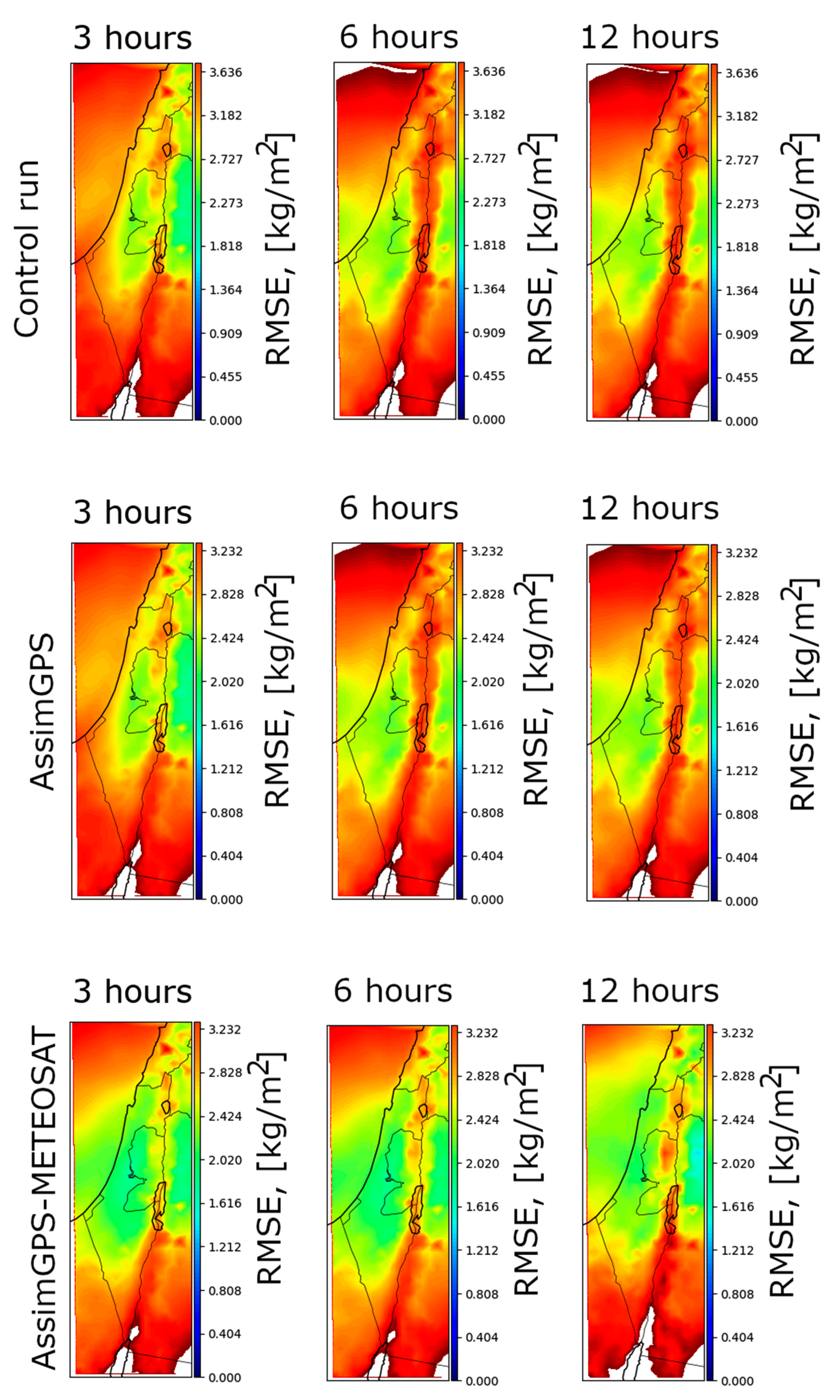
4.1. Verification of Control WRF Forecasts
4.2. Verification of AssimGPS Forecasts
4.3. Verification of AssimGPS-METEOSAT Forecasts
4.4. Verification of AssimGPS and AssimGPS-METEOSAT by Using 2D GPS IWV Maps
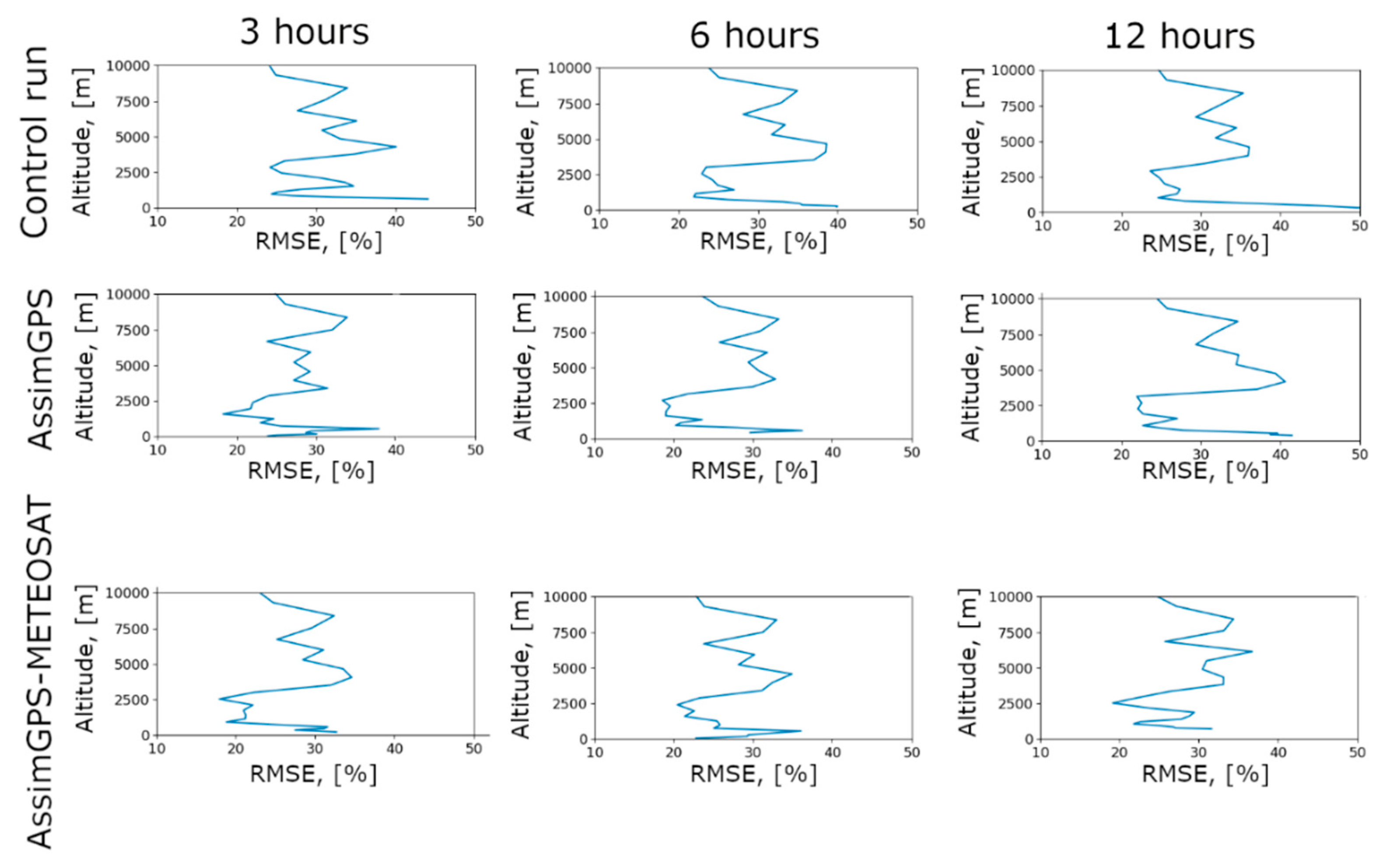
4.5. Verification of AssimGPS and AssimGPS-Meteosat versus Vertical Profile of Relative Humidity
5. Discussion and Conclusions
Author Contributions
Funding
Institutional Review Board Statement
Informed Consent Statement
Data Availability Statement
Conflicts of Interest
References
- Ehhalt, D.; Prather, M.; Dentener, F.; Derwent, R.; Dlugokencky, E.J.; Holland, E.; Isaksen, I.; Katima, J.; Kirchhoff, V.; Matson, P.; et al. Atmospheric chemistry and greenhouse gases. In Climate Change 2001: Impacts, Adaptation and Vulnerability; Maccarthy, J.J., Canziani, O.F., Leary, N.A., Eds.; Cambridge University Press: New York, NY, USA, 2001; pp. 241–287. [Google Scholar]
- Bevis, M.; Businger, S.; Chiswell, S.; Herring, T.A.; Anthes, R.A.; Rocken, C.; Ware, R.H. GPS Meteorology: Mapping Zenith Wet Delays onto Precipitable Water. J. Appl. Meteorol. 1994, 33, 379–386. [Google Scholar] [CrossRef]
- Bevis, M.; Businger, S.; Herring, T.A.; Rocken, C.; Anthes, R.A.; Ware, R.H. GPS meteorology: Remote sensing of atmospheric water vapor using the global positioning system. J. Geophys. Res. 1992, 97, 15787–15801. [Google Scholar] [CrossRef]
- Bosilovich, M.G.; Schubert, S.D. Water Vapor Tracers as Diagnostics of the Regional Hydrologic Cycle. J. Hydrometeor. 2002, 3, 149–165. [Google Scholar] [CrossRef]
- Yan, X.; Ducrocq, V.; Poli, P.; Hakam, M.; Jaubert, G.; Walpersdorf, A. Impact of GPS zenith delay assimilation on convective-scale prediction of Mediterranean heavy rainfall. J. Geophys. Res. Space Phys. 2009, 114, 3104. [Google Scholar] [CrossRef]
- Skamarock, W.C.; Klemp, B.J.; Dudhia, J.; Gill, D.O.; Barker, D.M.; Duda, M.G.; Huang, X.-Y.; Wang, W.; Powers, J.G. A Description of the Advanced Research WRF Version 3; NCAR Tech. Note, NCAR/TN-468+STR; National Center for Atmospheric Research: Boulder, CO, USA, 2008. [Google Scholar] [CrossRef]
- Skamarock, W.C.; Klemp, J.B.; Dudhia, J.; Gill, D.O.; Liu, Z.; Berner, J.; Wang, W.; Powers, J.G.; Duda, M.G.; Barker, D.M.; et al. A Description of the Advanced Research WRF Version 4; No. NCAR/TN-556+STR, NCAR Technical Note; National Center for Atmospheric Research: Boulder, CO, USA, 2019; 145p. [Google Scholar] [CrossRef]
- Kley, D.; Stone, E.; Henderson, W. SPARC Assessment of Upper Tropospheric and Stratospheric Water Vapor; WCRP 113, WMO/TD-1043, SPARC Rep. 2; World Clim. Res. Program: Geneva, Switzerland, 2000; p. 312. [Google Scholar]
- Miloshevich, L.M.; Vömel, H.; Whiteman, D.N.; Lesht, B.M.; Schmidlin, F.J.; Russo, F. Absolute accuracy of water vapor measurements from six operational radiosonde types launched during AWEX-G and implications for AIRS validation. J. Geophys. Res. 2006, 111, D09S10. [Google Scholar] [CrossRef]
- Soden, B.; Turner, D.D.; Lesht, B.M.; Miloshevich, L.M. An analysis of satellite, radiosonde, and lidar observations of upper tropospheric water vapor from the Atmospheric Radiation Measurement Program. J. Geophys. Res. Space Phys. 2004, 109. [Google Scholar] [CrossRef]
- Seidel, D.J.; Ross, R.J.; Angell, J.K.; Reid, G.C. Climatological characteristics of the tropical tropopause as revealed by radiosondes. J. Geophys. Res. 2001, 106, 7857–7878. [Google Scholar] [CrossRef]
- Wdowinski, S.; Eriksson, S. Geodesy in the 21st Century. Eos 2009, 90, 153–155. [Google Scholar] [CrossRef]
- Duan, J.; Bevis, M.; Fang, P.; Bock, Y.; Chiswell, S.; Businger, S.; Rocken, C.; Solheim, F.; van Hove, T.; Ware, R.; et al. GPS Meteorology: Direct Estimation of the Absolute Value of Precipitable Water. J. Appl. Meteorol. 1996, 35, 830–838. [Google Scholar] [CrossRef]
- Thayer, G.D. An improved equation for the radio refractive index of air. Radio Sci. 1974, 9, 803–807. [Google Scholar] [CrossRef]
- Moore, A.W.; Small, I.J.; Gutman, S.I.; Bock, Y.; Dumas, J.L.; Fang, P.; Haase, J.S.; Jackson, M.E.; Laber, J.L. National Weather Service Forecasters Use GPS Precipitable Water Vapor for Enhanced Situational Awareness during the Southern California Summer Monsoon. Bull. Am. Meteorol. Soc. 2015, 96, 1867–1877. [Google Scholar] [CrossRef]
- Shangguan, M.; Heise, S.; Bender, M.; Dick, G. Validation of GPS Atmospheric Water Vapor with WVR Data in Satellite Tracking Mode, 2015. Available online: http://eprints.uni-kiel.de/26354/ (accessed on 6 January 2020).
- Heise, S.; Dick, G.; Gendt, G.; Schmidt, T. Integrated Water Vapor from IGS Ground-Based GPS Observations: Initial Results from a Global 5-min Data Set. 2009. Available online: http://gfzpublic.gfz-potsdam.de/pubman/item/escidoc:239433:1/component/escidoc:239432/13798.pdf (accessed on 15 September 2020).
- Dai, A.; Wang, J.; Ware, R.H.; Van Hove, T. Diurnal variation in water vapor over North America and its implications for sampling errors in radiosonde humidity. J. Geophys. Res. 2002, 107, 4090. [Google Scholar] [CrossRef]
- Ohtani, R.; Naito, I. Comparisons of GPS-derived precipitable water vapors with radiosonde observations in Japan. J. Geophys. Res. Space Phys. 2000, 105, 26917–26929. [Google Scholar] [CrossRef]
- Liou, Y.A.; Teng, Y.T.; Hove, T.V.; Liljegren, J.C. Comparison of precipitable water observations in the near tropics by GPS, microwave radiometer, and radiosondes. J. Appl. Meteorol. 2001, 40, 5–15. [Google Scholar] [CrossRef]
- Vaquero-Martínez, J.; Antón, M.; Ortiz de Galisteo, J.P.; Cachorro, V.E.; Costa, M.J.; Román, R.; Bennouna, Y.S. Validation of MODIS integrated water vapor product against reference GPS data at the Iberian Peninsula. Int. J. Appl. Earth Obs. Geoinf. 2017, 63, 214–221. [Google Scholar] [CrossRef][Green Version]
- Bock, O.; Bouin, M.N.; Walpersdorf, A.; Lafore, J.P.; Janicot, S.; Guichard, F.; Agusti-Panareda, A. Comparison of ground-based GPS precipitable water vapour to independent observations and NWP model reanalyses over Africa. Q. J. R. Meteorol. Soc. 2007, 133, 2011–2027. [Google Scholar] [CrossRef]
- Song, S.; Zhu, W.; Ding, J.; Peng, J. 3D water-vapor tomography with Shanghai GPS network to improve forecasted moisture field. Chin. Sci. Bull. 2006, 51, 607–614. [Google Scholar] [CrossRef]
- Gendt, G.; Dick, G.; Reigber, C.; Tomassini, M.; Liu, Y.; Ramatschi, M. Near Real Time GPS Water Vapor Monitoring for Numerical Weather Prediction in Germany. J. Meteorol. Soc. Jpn. 2004, 82, 361–370. [Google Scholar] [CrossRef]
- Stone Smith, T.L.; Benjamin, S.G.; Gutman, S.I.; Sahm, S. Short-Range Forecast Impact from Assimilation of GPS-IPW Observations into the Rapid Update Cycle. Mon. Weather Rev. 2007, 135, 2914–2930. [Google Scholar] [CrossRef]
- Kumar, P.; Gopalan, K.; Shukla, B.P.; Shyam, A. Impact of single-point GPS integrated water vapor estimates on short-range WRF model forecasts over southern India. Theor. Appl. Clim. 2016, 130, 755–760. [Google Scholar] [CrossRef]
- Lagasio, M.; Pulvirenti, L.; Parodi, A.; Boni, G.; Pierdicca, N.; Venuti, G.; Realini, E.; Tagliaferro, G.; Barindelli, S.; Rommen, B. Effect of the ingestion in the WRF model of different Sentinel-derived and GNSS-derived products: Analysis of the forecasts of a high impact weather event. Eur. J. Remote Sens. 2019, 52, 16–33. [Google Scholar] [CrossRef]
- Velden, C.S.; Hayden, C.M.; Nieman, S.J.; Menzel, W.P.; Wanzong, S.; Goerss, J.S. Upper-Tropospheric Winds Derived from Geostationary Satellite Water Vapor Observations. 1997. Available online: http://ntrs.nasa.gov/search.jsp?R=19980018993 (accessed on 20 June 2020).
- Cresswell, M.; Morse, A.; Thomson, M. Estimating surface air temperatures, from Meteosat land surface temperatures, using an empirical solar zenith angle model. Int. J. Remote. Sens. 1999, 20, 1125–1132. [Google Scholar] [CrossRef]
- Jiang, J.H.; Su, H.; Zhai, C.; Perun, V.S.; Del Genio, A.; Nazarenko, L.S.; Donner, L.J.; Horowitz, L.; Seman, C.; Cole, J.; et al. Evaluation of cloud and water vapor simulations in CMIP5 climate models using NASA “A-Train” satellite observations. J. Geophys. Res. Atmos. 2012, 117, D14105. [Google Scholar] [CrossRef]
- Leontiev, A.; Reuveni, Y. Combining Meteosat-10 satellite image data with GPS tropospheric path delays to estimate regional integrated water vapor (IWV) distribution. Atmos. Meas. Tech. 2017, 10, 537–548. [Google Scholar] [CrossRef]
- Leontiev, A.; Reuveni, Y. Augmenting GPS IWV estimations using spatio-temporal cloud distribution extracted from satellite data. Sci. Rep. 2018, 8, 14785. [Google Scholar] [CrossRef] [PubMed]
- Boehm, J.; Werl, B.; Schuh, H. Troposphere mapping functions for GPS and very long baseline interferometry from European Centre for Medium-Range Weather Forecasts operational analysis data. J. Geophys. Res. Solid Earth 2006, 111, B02406. [Google Scholar] [CrossRef]
- Reuveni, Y.; Bock, Y.; Tong, X.; Moore, A.W. Calibrating interferometric synthetic aperture radar (InSAR) images with regional GPS network atmosphere models. Geophys. J. Int. 2015, 202, 2106–2119. [Google Scholar] [CrossRef]
- Reuveni, Y.; Kedar, S.; Moore, A.; Webb, F. Analyzing slip events along the Cascadia margin using an improved subdaily GPS analysis strategy. Geophys. J. Int. 2014, 198, 1269–1278. [Google Scholar] [CrossRef]
- Reuveni, Y.; Kedar, S.; Owen, S.E.; Moore, A.W.; Webb, F.H. Improving sub-daily strain estimates using GPS measurements. Geophys. Res. Lett. 2012, 39. [Google Scholar] [CrossRef]
- Gaete, K.; Carrasco, J.; Jaña, R.; Sepúlveda, H. A Sensitivity Analysis of the WRF Model in Climate Simulation for an Area in Fuego-Patagonia. 2019. Available online: https://www.researchgate.net/publication/335172852_A_sensitivity_analysis_of_the_WRF_model_in_climate_simulation_for_an_area_in_Fuego-Patagonia (accessed on 6 July 2020).
- Khain, A.; Pinsky, M. Physical Processes in Clouds and Cloud Modeling; Cambridge University Press: Cambridge, UK, 2018. [Google Scholar] [CrossRef]
- Lynn, B.H.; Khain, A.; Dudhia, J.; Rosenfeld, D.; Pokrovsky, A.; Seifert, A. Spectral (Bin) Microphysics Coupled with a Mesoscale Model (MM5). Part I: Model Description and First Results. Mon. Weather Rev. 2005, 133, 44–58. [Google Scholar] [CrossRef]
- Roh, W.; Satoh, M. Evaluation of Precipitating Hydrometeor Parameterizations in a Single-Moment Bulk Microphysics Scheme for Deep Convective Systems over the Tropical Central Pacific. J. Atmos. Sci. 2014, 71, 2654–2673. [Google Scholar] [CrossRef]
- Dudhia, J. Numerical Study of Convection Observed during the Winter Monsoon Experiment Using a Mesoscale Two-Dimensional Model. J. Atmos. Sci. 1989, 46, 3077–3107. [Google Scholar] [CrossRef]
- Mlawer, E.J.; Taubman, S.J.; Brown, P.D.; Iacono, M.J.; Clough, S.A. Radiative transfer for inhomogeneous atmospheres: RRTM, a validated correlated-k model for the longwave. J. Geophys. Res. Space Phys. 1997, 102, 16663–16682. [Google Scholar] [CrossRef]
- Hong, S.; Noh, Y.; Dudhia, J. A New Vertical Diffusion Package with an Explicit Treatment of Entrainment Processes. Mon. Weather Rev. 2006, 134, 2318–2341. [Google Scholar] [CrossRef]
- Zhao, J.; Guo, Z.-H.; Su, Z.-Y.; Zhao, Z.-Y.; Xiao, X.; Liu, F. An improved multi-step forecasting model based on WRF ensembles and creative fuzzy systems for wind speed. Appl. Energy 2016, 162, 808–826. [Google Scholar] [CrossRef]
- Fisher, M. Background error covariance modelling. In Proceedings of the ECMWF Seminar on Recent Development in Data Assimilation for Atmosphere and Ocean, Reading, UK, 8–12 September 2003; pp. 45–63. [Google Scholar]
- Sun, Q.; Vihma, T.; Jonassen, M.O.; Zhang, Z. Impact of Assimilation of Radiosonde and UAV Observations from the Southern Ocean in the Polar WRF Model. Adv. Atmos. Sci. 2020, 37, 441–454. [Google Scholar] [CrossRef]
- Yang, J.; Duan, K.; Wu, J.; Qin, X.; Shi, P.; Liu, H.; Xie, X.; Zhang, X.; Sun, J. Effect of Data Assimilation Using WRF-3DVAR for Heavy Rain Prediction on the Northeastern Edge of the Tibetan Plateau. Adv. Meteorol. 2015, 294589. [Google Scholar] [CrossRef]
- Hacker, J.; Draper, C.; Madaus, L. Challenges and Opportunities for Data Assimilation in Mountainous Environments. Atmosphere 2018, 9, 127. [Google Scholar] [CrossRef]
- Hanna, N.; Trzcina, E.; Moeller, G.; Rohm, W.; Weber, R. Assimilation of GNSS tomography products into WRF using radio occultation data assimilation operator. Atmos. Meas. Tech. Discuss. 2019, 1–32. [Google Scholar] [CrossRef]
- Rohm, W.; Guzikowski, J.; Wilgan, K.; Kryza, M. 4DVAR assimilation of GNSS zenith path delays and precipitable water into a numerical weather prediction model WRF. Atmos. Meas. Tech. 2019, 12, 345–361. [Google Scholar] [CrossRef]
- Colle, B.; Westrick, K.J.; Mass, C. Evaluation of MM5 and Eta-10 precipitation forecasts over the Pacific Northwest during the cool season. Weather Forecast. 1999, 14, 137–153. [Google Scholar] [CrossRef]
- Zhong, S.; Fast, J.D. An Evaluation of the MM5, RAMS, and Meso-Eta Models at Subkilometer Resolution Using VTMX Field Campaign Data in the Salt Lake Valley. Mon. Weather Rev. 2003, 131, 1301–1322. [Google Scholar] [CrossRef]
- Zhong, S.; In, H.-J.; Bian, X.; Charney, J.; Heilman, W.; Potter, B. Evaluation of Real-Time High-Resolution MM5 Predictions over the Great Lakes Region. Weather Forecast. 2005, 20, 63–81. [Google Scholar] [CrossRef]
- Ziskin, S.; Yair, Y.; Alpert, P.; Uzan, L.; Reuveni, Y. The diurnal variability of precipitable water vapor derived from GPS tropospheric path delays over the Eastern Mediterranean. Atmos. Res. 2021, 249, 105307. [Google Scholar] [CrossRef]
- Kunin, P.; Alpert, P.; Rostkier-Edelstein, D. Investigation of sea-breeze/foehn in the Dead Sea valley employing high resolution WRF and observations. Atmos. Res. 2019, 229, 240–254. [Google Scholar] [CrossRef]


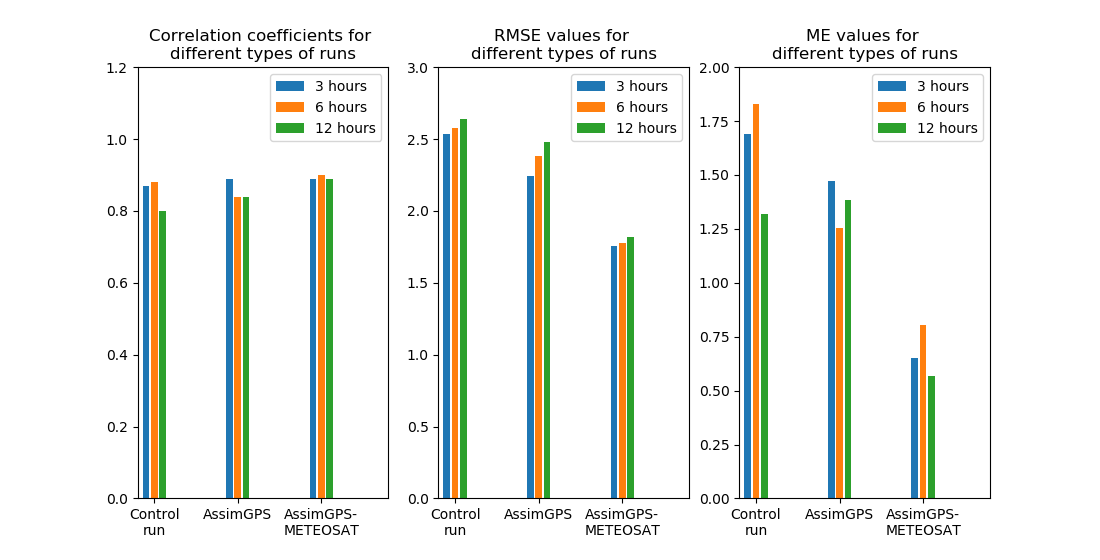
| 3 h | 6 h | 12 h | |
|---|---|---|---|
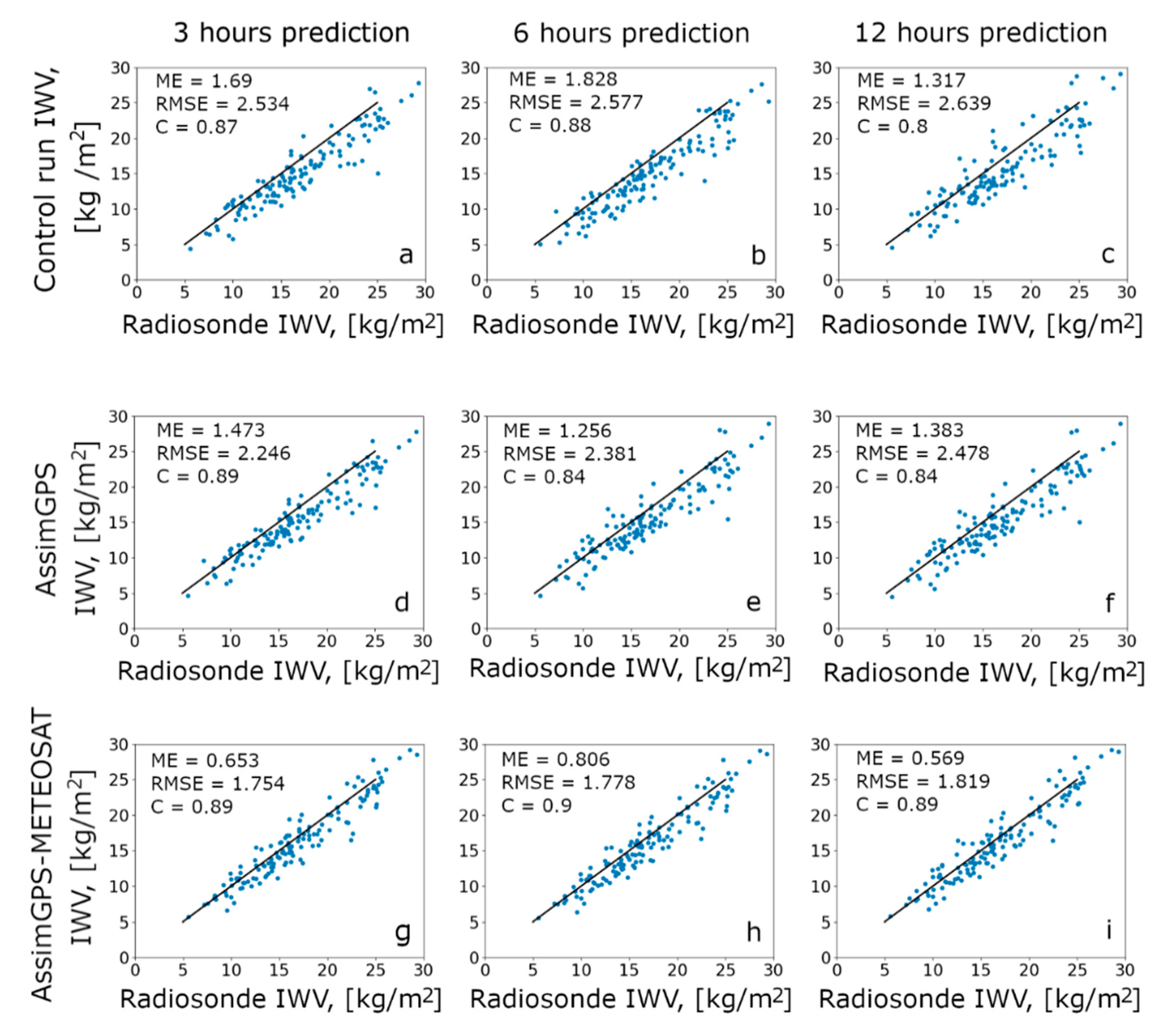
| 1. Control | |||
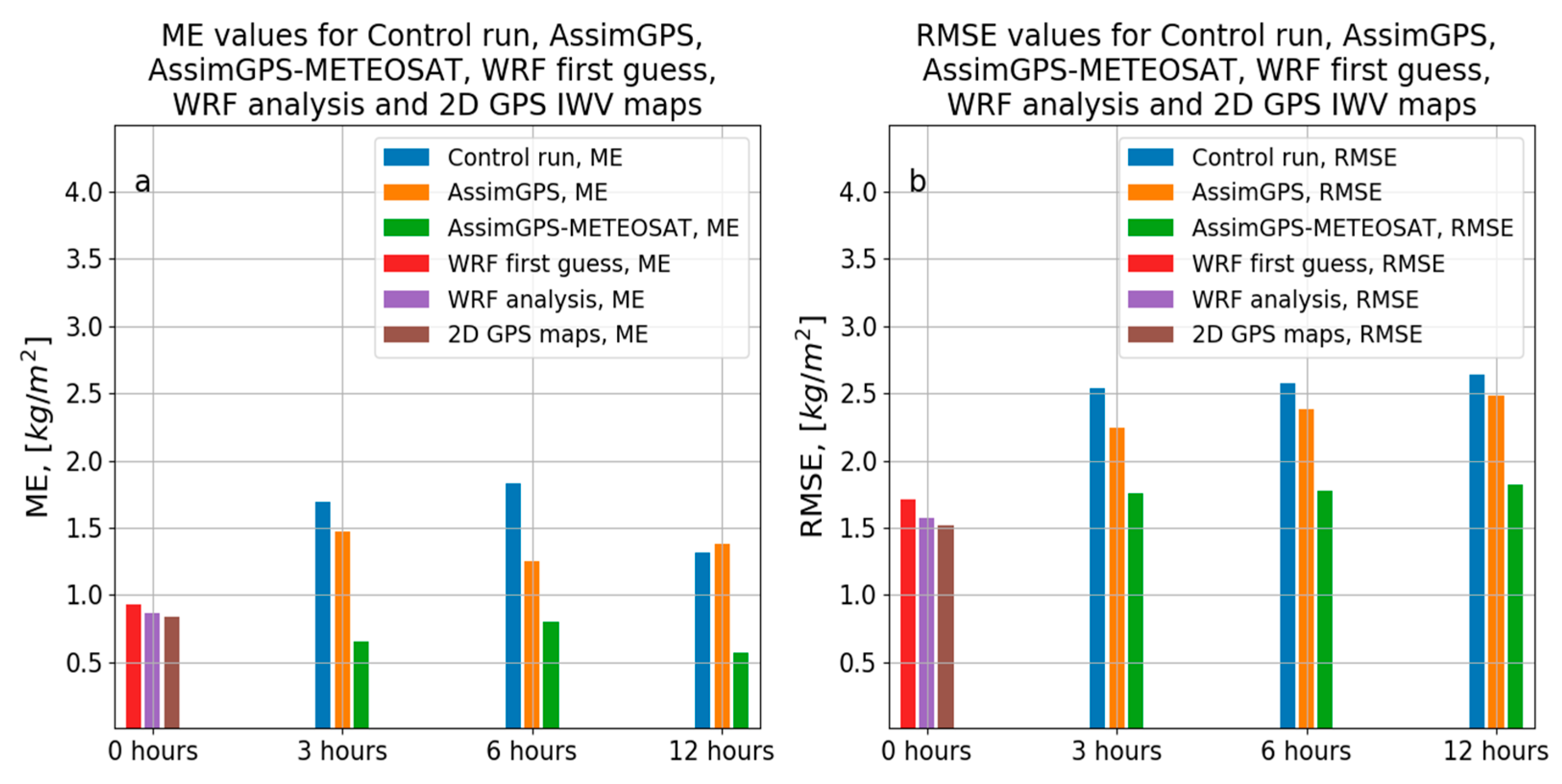
| RMSE, mm | 2.534, (0.439, 0.437) | 2.577, (0.429, 0.434) | 2.639, (0.332, 0.323) |
| ME, mm | 1.69 | 1.828 | 1.317 |
| C | 0.87 | 0.88 | 0.8 |
| 2. AssimGPS | |||
| RMSE, mm | 2.246, (0.291, 0.301) | 2.381, (0.299, 0.291) | 2.478, (0.266, 0.328) |
| ME, mm | 1.473 | 1.256 | 1.383 |
| C | 0.89 | 0.84 | 0.84 |
| Improvement of RMSE with respect to the Control run (%) | 11 | 7.5 | 6 |
| 3. AssimGPS-METEOSAT | |||
| RMSE. mm | 1.754, (0.235, 0.195) | 1.778, (0.210, 0.207) | 1.819, (0.262, 0.202) |
| ME, mm | 0.653 | 0.806 | 0.569 |
| C | 0.89 | 0.9 | 0.89 |
| Improvement of RMSE with respect to the control run (%) | 30 | 31 | 31 |
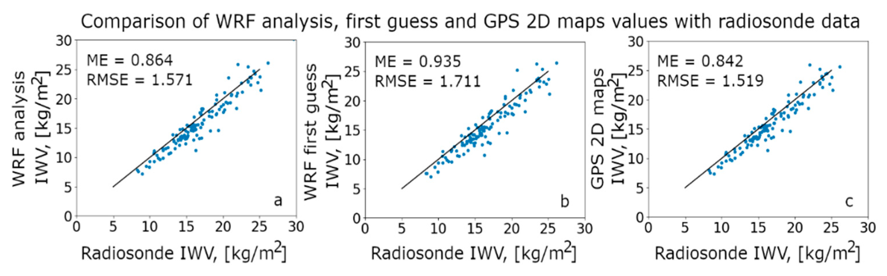
| ME, mm | RMSE, mm | |
|---|---|---|
| WRF first guess | 0.935 | 1.711 |
| WRF analysis | 0.864 | 1.571 |
| GPS IWV 2D maps | 0.842 | 1.519 |
Publisher’s Note: MDPI stays neutral with regard to jurisdictional claims in published maps and institutional affiliations. |
© 2020 by the authors. Licensee MDPI, Basel, Switzerland. This article is an open access article distributed under the terms and conditions of the Creative Commons Attribution (CC BY) license (http://creativecommons.org/licenses/by/4.0/).
Share and Cite
Leontiev, A.; Rostkier-Edelstein, D.; Reuveni, Y. On the Potential of Improving WRF Model Forecasts by Assimilation of High-Resolution GPS-Derived Water-Vapor Maps Augmented with METEOSAT-11 Data. Remote Sens. 2021, 13, 96. https://doi.org/10.3390/rs13010096
Leontiev A, Rostkier-Edelstein D, Reuveni Y. On the Potential of Improving WRF Model Forecasts by Assimilation of High-Resolution GPS-Derived Water-Vapor Maps Augmented with METEOSAT-11 Data. Remote Sensing. 2021; 13(1):96. https://doi.org/10.3390/rs13010096
Chicago/Turabian StyleLeontiev, Anton, Dorita Rostkier-Edelstein, and Yuval Reuveni. 2021. "On the Potential of Improving WRF Model Forecasts by Assimilation of High-Resolution GPS-Derived Water-Vapor Maps Augmented with METEOSAT-11 Data" Remote Sensing 13, no. 1: 96. https://doi.org/10.3390/rs13010096
APA StyleLeontiev, A., Rostkier-Edelstein, D., & Reuveni, Y. (2021). On the Potential of Improving WRF Model Forecasts by Assimilation of High-Resolution GPS-Derived Water-Vapor Maps Augmented with METEOSAT-11 Data. Remote Sensing, 13(1), 96. https://doi.org/10.3390/rs13010096