Abstract
Previous studies have reported that intra-urban variability of NO2 concentrations is even higher than inter-urban variability. In recent years, an increasing number of studies have developed satellite-derived land use regression (LUR) models to predict ground-level NO2 concentrations, though only a few have been conducted at a city scale. In this study, we developed a satellite-derived LUR model to predict seasonal NO2 concentrations at a city scale by including satellite-retrieved NO2 tropospheric column density, population density, traffic indicators, and NOx emission data. The R2 of model fitting and 10-fold cross validation were 0.70 and 0.61 for the satellite-derived seasonal LUR model, respectively. The satellite-based LUR model captured seasonal patterns and fine gradients of NO2 variations at a 100 m × 100 m resolution and demonstrated that NO2 pollution in winter is 1.46 times higher than that in summer. NO2 concentrations declined significantly with increasing distance from roads and with increasing distance from the city center. In Suzhou, 84% of the total population lived in areas with NO2 concentrations exceeding the annual-mean standard at 40 μg/m3 in 2014. This study demonstrated that satellite-retrieved data could help increase the accuracy and temporal resolution of the traditional LUR models at a city scale. This application could support exposure assessment at a high resolution for future epidemiological studies and policy development pertaining to air quality control.
1. Introduction
Nitrogen dioxide (NO2) is not only a primary pollutant mainly from fossil fuel emissions but also a secondary pollutant arising in large part from a photochemical conversion combining NO with O3 [1,2]. It is a common indicator for traffic-related air pollution and proven to be associated with a myriad of adverse health effects. NO2 has been positively linked to lung cancer mortality in California by the American Cancer Society Cancer Prevention II Study [3]. In China, short-term exposure to NO2 was significantly associated with total natural causes mortality and cardiorespiratory disease mortality across 272 cities [4]. Even at or below the current European Air quality limit values, the associations between NO2 exposure and adverse effects have been found for both short-term and long-term exposure in Europe [5]. In previous epidemiological studies, exposure to NO2 was mostly evaluated using ground-based fixed monitoring data, interpolation methods, or land use regression (LUR) models [6,7].
The concentrations of NO2 may decline at a distance of several hundred meters from emission sources [8], and the spatial distributions of NO2 differ significantly between, and especially within, cities [9,10]. In Canada, variations in NO2 concentrations within a city further showed a stronger association with cause-specific mortality than that between cities [11]. Thus, it is an essential issue to evaluate intra-urban NO2 concentrations with a high spatial resolution for epidemiological studies. The LUR models are one of the most common assessment methods used to capture spatial variability of NO2 with a high spatial resolution, and have been applied in NO2-related cohort studies in Europe and the United States [9,12,13,14,15]. Land use regression models also have been developed for predicting NO2 concentrations in Chinese cities, including Shanghai, Tianjin, and Wuhan [16,17,18]. Traditional LUR models highly depend on land use data and have lower temporal resolution, but these do not satisfy the flexible requirements of exposure assessment in epidemiological studies.
Satellite data have been proven to be one of the key predictors for estimating ambient NO2 concentrations with a high temporal resolution [19,20,21]. Specifically, a study in Western Europe indicated that the adjusted R2 of LUR models with satellite data was increased by 0.02–0.06 compared to the models without satellite data with the R2 of 0.48–0.56 [22]. Other studies showed that the satellite-based LUR models could expand the temporal resolution of traditional LUR models for predicting air pollutants’ concentrations, from annual level to monthly or seasonal scales [19,23,24,25]. NO2 column density from the Ozone Monitoring Instrument (OMI) aboard satellite Aura is the most commonly used dataset for establishing satellite-based LUR or machine learning models [26,27,28]. The satellite-based LUR models not only expanded the temporal resolution of traditional ones [19], but also simultaneously helped improve model performance [22,29,30]. However, in China, most of these studies were conducted at regional or national scales [21,31]; whether satellite data can improve the resolution and model performance of LUR models at a city scale, has not been fully evaluated. In addition, the row anomaly of OMI led to a large amount of missing data at the daily level [32], hence OMI NO2 column density data might be inappropriate to be directly used to assess NO2 exposure levels within a city at a daily scale, and some studies resampled the data at a seasonal scale [33].
Therefore, in this study, we developed a satellite-derived LUR model, in a Chinese metropolis, to capture intra-urban NO2 temporal variations at a seasonal level with a high spatial resolution. This model with a high spatial resolution is expected to capture the finer gradients of NO2 variations within a city at a higher temporal resolution than that of the traditional LUR model, which could provide more accurate exposure assessment for epidemiological studies.
2. Materials and Methods
2.1. Study Area
Suzhou is a city located in southeastern Jiangsu Province of East China (Figure 1). It includes five urban districts (Gusu, Huqiu, Wuzhong, Xiangcheng, and Wujiang) and four satellite cities (Changshu, Taicang, Kunshan, and Zhangjiagang). Suzhou is one of five urban locations in the China Kadoorie Biobank (CKB) cohort that have focused on common chronic diseases since 2004 [34]. We developed a satellite-derived LUR model in Suzhou as a case study to establish the methodology for the assessment of exposure to NO2 of the CKB cohort study to support the next phase of air pollution-related epidemiological studies. Suzhou covered 8488.42 km2 in 2018 and about 42.5% of the total area was covered by waterbody. The total registered population in Suzhou reached 7.04 million by the end of 2018 (http://tjj.suzhou.gov.cn/sztjj/tjnj/2019/zk/indexce.htm). Suzhou is located in a subtropical monsoon climate zone with four distinct seasons.
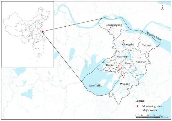
Figure 1.
The location of Suzhou in China and the NO2 monitoring sites in Suzhou that were used in this study.
2.2. Data
The database included data on NO2 monitoring, NO2 tropospheric column density from the OMI instrument, population density, road network, land use parameters, and NOx emissions.
2.2.1. Monitoring Data
Daily NO2 monitoring data of 20 fixed air quality stations were obtained from the National Environmental Monitoring Network, and the locations of the stations are shown in Figure 1. In accordance with the Chinese Ambient Air Quality Standard (GB3095-2012), at least 20 hourly measurements were included to calculate the daily NO2 concentration; at least 27 daily values were needed to calculate monthly concentrations (25 daily values for February); at least 324 daily values were needed to calculate the annual concentration. Most of the fixed stations were located in areas with a relatively high population density to represent the averaged exposure levels for public health.
2.2.2. Satellite Data
The OMI instrument is on board the National Aeronautics and Space Administration (NASA) Aura satellite that was launched in 2004. It measures radiances across 270–500 nm of the ultraviolet and visible waveband. Global tropospheric vertical column NO2 density data of OMI level 2 (OMNO2) product, with a spatial resolution of 13 km × 24 km at nadir [35], are available online at a daily time step and were downloaded from NASA Goddard Earth Sciences Data and Information Services Center (https:// earthdata.nasa.gov/). Cloud cover and a dynamic row anomaly problem of OMI were responsible for a significantly high rate of missing values of daily data. The “row anomaly” occurred due to the technical issues of the OMI, which has produced invalid data in the center-right part of each swath of observations since 2008 [32]. Within a city, the high missing rate might cause low availability of OMI NO2 tropospheric column density data at a daily level. Therefore, seasonal resampling was done by averaging all daily OMI NO2 tropospheric column density data falling inside a 40 km × 40 km grid to fill the gap caused by missing data and smooth the noise [33]. The satellite data were then interpolated to the fixed monitoring stations using an inverse distance weighted (IDW) method.
2.2.3. Other Predictors
Land Use Parameters
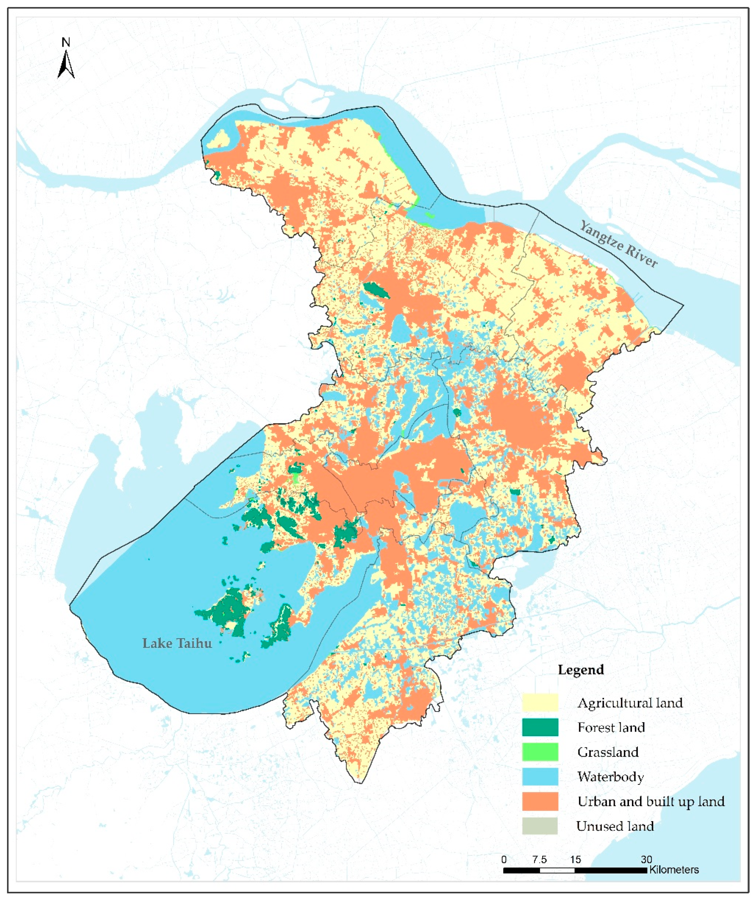
Land use data (agricultural, forest, grassland, waterbody, urban and built up, and unused land) from 2014 were interpreted from the Landsat TM5 dataset (https://earthexplorer.usgs.gov/) with a 30 m spatial resolution (Figure 2). Specifically, agricultural land included dry land and paddy fields; forest land included dense forests, shrub forests, loose forests, and other forests; grassland included highly-covered grassland; waterbody included rivers, lakes, beaches, bottomlands, and reservoirs; urban and built up land included urban and rural settlements and other built-up land; unused land included bare rock and sand. In Suzhou, the major land use types were urban and built-up land, agricultural land, and waterbody; and agricultural land mainly consisted of paddy fields. To optimize the correlation between NO2 measurements and land use predictors, different buffer distances were applied, from 100 m to 5000 m, at 100-m intervals, around the 20 fixed monitoring sites [10,17,36]. The areas of each land use type were then calculated within these buffer zones separately.
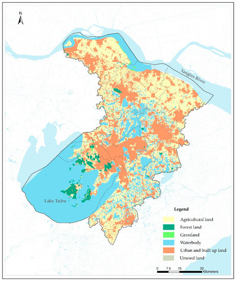
Figure 2.
The spatial distribution of types of land use in this study in Suzhou in 2014.
Road Network
Lengths of major roads and distances to the nearest major road were calculated as indicators of traffic emissions. Types of roads included expressways, national roads, provincial roads, urban expressways, county roads, town roads, and other roads. Then, expressways, national roads, provincial roads, and urban expressways were merged as major roads. Within the buffers from 100 m to 5000 m (at 100 m intervals) around the 20 fixed monitoring sites, the lengths of major roads were then calculated [6,17]. Distance from monitoring sites to the nearest major road, inverse of the distance, and logarithmic transformation of the inverse distance were also calculated as indicators of traffic emissions [6,10].
Population Density
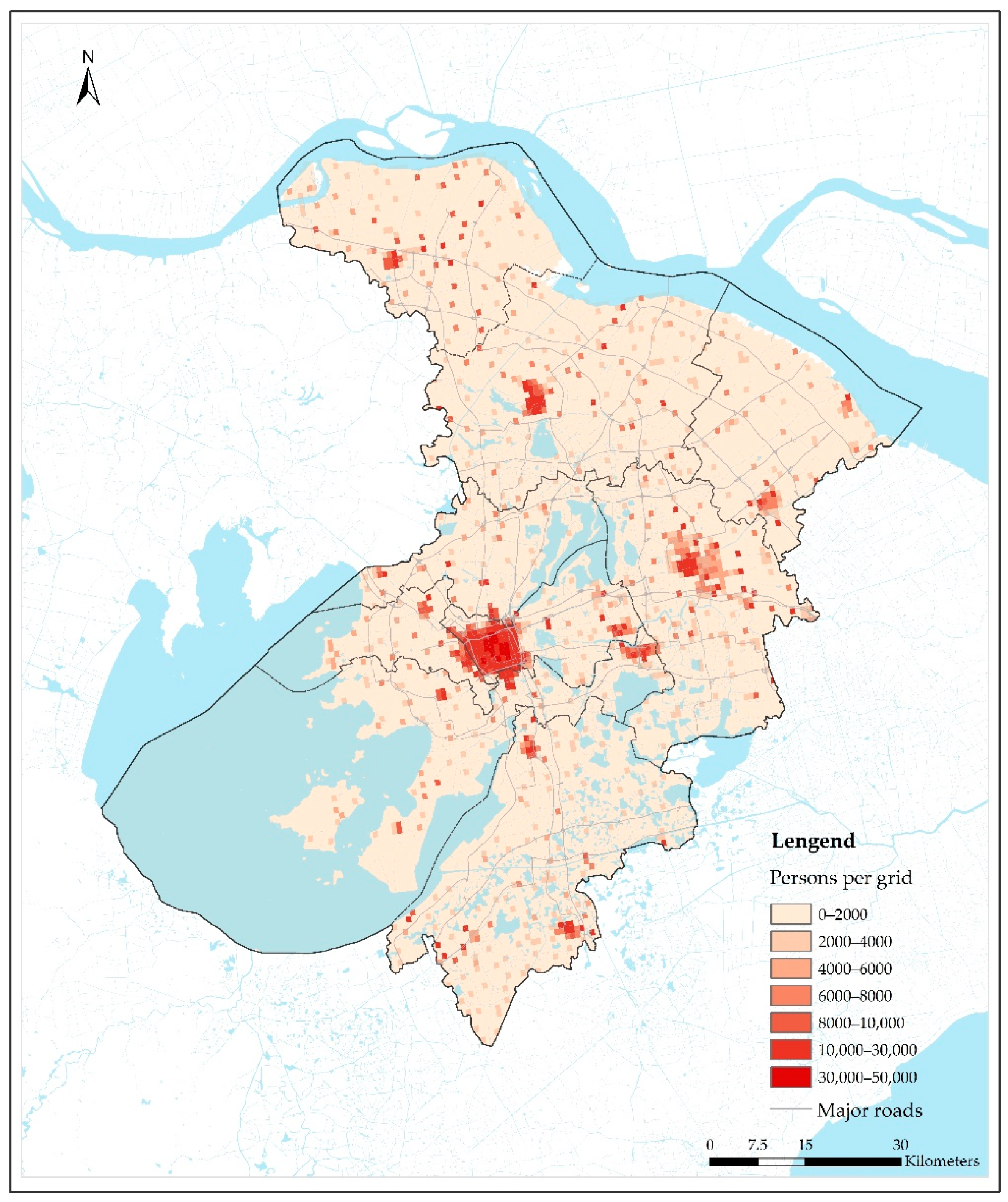
Population density data were obtained from the Oak Ridge National Laboratory (ORNL)’s LandScan 2014 global database at 30″ × 30″ resolution in raster format (http://www.ornl.gov/sci/landscan/), which were then interpolated to the NO2 monitoring stations using the IDW method. The population data, with an ESRI binary raster format, is approximately at a 1 km × 1 km resolution and each grid represents an average population number within the grid at an annual level (https://landscan.ornl.gov/documentation). Figure 3 shows the spatial distribution of the population in Suzhou in 2014, suggesting that more people tended to live in the center of five urban districts and four satellite cities in Suzhou.

Figure 3.
The distribution of population and major roads in Suzhou.
NOx Emissions
NOx emission inventory data were collected from the Multiresolution Emission Inventory of China (MEIC, http://www.meicmodel.org) at a spatial resolution of 1 km × 1 km. The industrial NO2 emissions from power plants and non-power plants were computed separately within buffer zones of 1 km to 10 km, at 1-km intervals, around each monitoring site.
2.3. Model Development and Evaluation
A traditional LUR model was developed, as the first step, to select the most optimized predictors from all parameters with a linear regression model [6,10,20,36]. Since the OMI NO2 tropospheric column density was aggregated at a seasonal level to fill the gap caused by the high missing rate of the satellite data [32], this model was developed at a seasonal level [37,38]. First, we set every potential variable a prior direction. Second, manual backward supervised regression was conducted based on NO2 seasonal concentrations to select the most optimized predictor variables. Predictors were kept in the model if they satisfied the criteria proposed by previous studies [6,10,17]: (1) the variables improved the model R2 by at least 1%; (2) the effect directions of the variables were consistent with the prior directions; (3) the variables that were already in the model did not change their effect directions; (4) the variable would be excluded from the model if the p value was less than 0.1. This process continued until there were no more variables meeting the criteria. Variance inflation factors (VIFs) were calculated as an indicator of multicollinearity. Variables with VIF values greater than three were removed from the satellite-based LUR model and this step was repeated.
In the second step, a linear mixed effects model was developed (see Equation (1)) by involving random effects of OMI NO2 tropospheric column density [23,37]. The advantage of employing this model was to include the variability of associations between NO2 concentrations and OMI NO2 tropospheric column density over time. Similar satellite-based models had been developed for predicting PM2.5 concentrations in a national assessment [37] and PM10 concentrations within a city in Shanghai [23]. In this model, the OMI NO2 tropospheric column density had both random effect and fixed effect coefficients, which represented seasonal variability in the association between NO2 measurements and OMI NO2 tropospheric column density and the average effect of satellite measurements on the ground NO2 measurements for the whole year, respectively [23,37]. The model structure can be summarized as:
where NO2,st indicates the mean observed NO2 concentrations (μg/m3) at the fixed station s in season t; OMIst is the only independent variable with both fixed and random effects, which represents OMI NO2 tropospheric column density data at the fixed station s in season t; β0 and β0’ are the intercepts of the fixed and season-specific random effects for the model, respectively; β1 and β1’indicate the fixed and season-specific random slopes for OMIst, respectively; Xis represents a series of predictors, which are selected by satisfying the criteria from the first step; and βis represents the fixed slope for predictor i at the fixed station s; and εst is the error term at the fixed station s in season t.
NO2,st = (β0 + β0’) + (β1 + β1’) OMIst + βisXis + εst
In the third step, 10-fold cross validation (CV) was applied to evaluate the model performance [17,37]: 90% of the data were randomly selected for model development, which was used to predict NO2 concentrations of the remaining 10% of the data; and this process was repeated 10 times. Root mean squared error (RMSE) was calculate as the standard deviation of the residuals. RMSE and R2 were used to evaluate the model’s performance by comparing measured and predicted NO2 concentrations during model development and 10-fold CV, respectively. The relative prediction error (RPE, defined as RMSE divided by the mean NO2 measurements) from 10-fold CV was then calculated to evaluate prediction accuracy.
In the fourth step, seasonal prediction maps of NO2 concentrations in Suzhou were produced based on the satellite-derived LUR models, at a 100 m × 100 m resolution at a seasonal timescale. In addition, we further calculated annual-mean and seasonal-mean population-weighted NO2 concentrations in Suzhou [39] (see Equation (2)).
where CPop indicates the annual-mean or seasonal-mean population-weighted NO2 exposure concentrations in Suzhou; Popi represents the population density of grid i; and Ci indicates the estimated annual-mean or seasonal-mean NO2 concentrations of grid i.
CPop = ∑Popi × Ci/∑Popi
Figure 4 shows the workflow for the development of the satellite-derived LUR model in our study. Statistical analyses were performed with nlme packages (https://www.rdocumentation.org/packages/nlme/versions/3.1-151/topics/nlme) of R3.6.1.
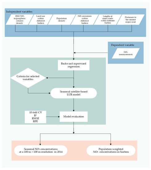
Figure 4.
Workflow for the development of the satellite-derived LUR model.
3. Results
3.1. Descriptive Statistics Analyses
In 2014, the annual-mean NO2 was 46.23 μg/m3 in Suzhou, with the lowest concentration of 36.52 μg/m3 recorded in summer and the highest concentration of 53.22 μg/m3 in winter, as measured at fixed monitoring sites. Among all predictors, the Pearson’s correlation coefficient between seasonal OMI NO2 tropospheric column density and seasonal NO2 measurements was highest with the value of 0.65.
3.2. Model Development and Evaluation
After variable selection, as the results of the first step, the satellite-derived LUR model included four predictors: NO2 tropospheric column density from OMI, population density, log transformed inverse of nearest distances to major roads (Log_distance), and NO2 non-power plants emissions within a 10-km buffer zone (Table 1). The R2 and RMSE of this model were 0.63 and 5.76 μg/m3, respectively. The R2 and RMSE of the 10-fold CV were 0.59 and 6.09 μg/m3, respectively. The VIFs of the four variables were all less than 2, showing weak multicollinearity among them.

Table 1.
The traditional land use regression (LUR) model for predicting NO2 concentrations.
The results of the second step, including the estimated coefficients of fixed effects of the four predictor variables, are shown in Table 2. All predictors were positively and significantly associated with measured NO2 concentrations, with p values less than 0.05. The absolute contribution (IQR × β), for each influencing predictor, was calculated as the regression coefficient (β) of fixed effects multiplied by the inter-quartile range (IQR) of the corresponding predictor. The results indicated that the non-power emissions within a 10-km buffer zone and OMI NO2 tropospheric column density contributed most to NO2 concentrations, because they had higher IQR × β values (Table 2).

Table 2.
The fixed effects of the satellite-derived LUR model for predicting NO2 concentrations.
The R2 and RMSE of the seasonal satellite-derived LUR model were 0.70 and 5.24 μg/m3, respectively. The R2 and RMSE of the 10-fold CV were 0.61 and 5.91 μg/m3, respectively, for the seasonal model (Figure 5). The RPE from 10-fold CV was 12.78%, which indicated a relatively high predicting accuracy at the seasonal level. The linear mixed effects model performed better than the traditional linear regression model, suggesting the importance of considering the seasonal variability of the association between ground NO2 measurements and OMI NO2 tropospheric column density.
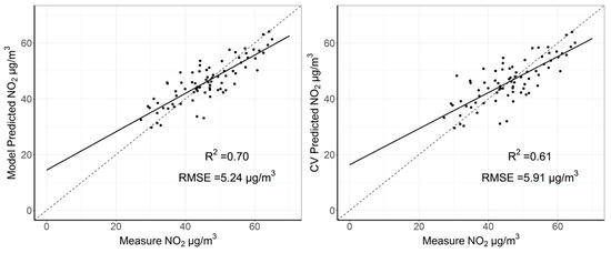
Figure 5.
Scatter plots of measured and predicted NO2 concentrations from model fitting (left), and 10-fold cross validation (right), respectively, for the satellite-derived linear mixed effects model at a seasonal timescale.
3.3. Spatiotemporal Trends of Predicting NO2 Concentrations
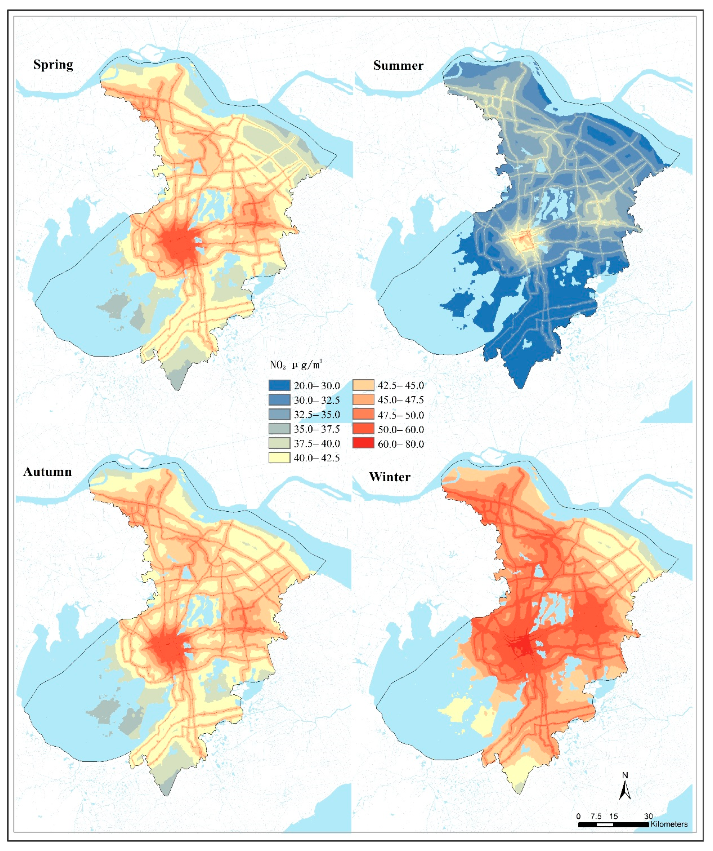
Predictive maps of NO2 concentrations with a spatial resolution of 100 m × 100 m were produced at a seasonal timescale (Figure 6). The seasonal pattern of predicted NO2 concentrations agreed well with field measurements. Mean NO2 concentration was highest in winter (47.3 μg/m3) in Suzhou, which was 1.46 times higher than that in summer. The spatial patterns of NO2 predictions were similar at different seasons throughout the year. Maps with high spatial resolution showed that severe NO2 pollution occurred along the major roads and declined significantly with increasing distance from the road. Urban centers with high population density and an intensive road network also experienced higher NO2 concentrations than that of the rural areas (Figure 6). For example, in summer, the maximum NO2 concentration (58.99 μg/m3) that occurred in urban areas was 2.77 times higher than the minimum value (21.33 μg/m3) in rural areas; and in winter, the maximum concentration (76.93 μg/m3) was 2.03 times higher compared to the lowest value (37.91 μg/m3) in rural areas. The results indicated that the NO2 concentration was generally higher in urban areas than that in rural areas both in winter and summer.
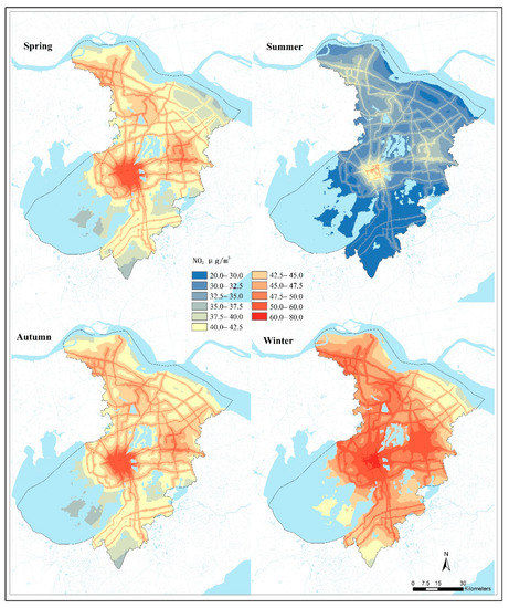
Figure 6.
NO2 spatial distribution at the seasonal level in Suzhou, 2014.
The population-weighted annual mean NO2 concentration in 2014 was 44.94 μg/m3 in Suzhou, higher than the annual-mean predicted concentration of 41.4 μg/m3 and also higher than the annual-mean NO2 standard of 40 μg/m3 defined in the Chinese National Ambient Air Quality Standards (GB 3095-2012). In winter, 99% of the total population lived in areas with NO2 concentrations exceeding 40 μg/m3 in Suzhou (Table 3).

Table 3.
Population-weighted NO2 exposure concentrations.
4. Discussion
Our study built a satellite-derived LUR model with OMI NO2 tropospheric column density data to predict NO2 concentrations at seasonal timescales with a high spatial resolution (100 m × 100 m) in Suzhou. The R2 values of model fitting and 10-fold CV were 0.70 and 0.61 at seasonal timescales, respectively, reflecting the relatively high stability of the model.
Our seasonal satellite-derived LUR model performance was comparable with previous satellite-based LUR models on NO2 concentration assessment at global, national, and regional scales. For the global satellite-based LUR model, the R2 and MAE (mean absolute error) for the model were 0.54 and 3.7 ppb at a 100 m×100 m resolution, respectively [20]. The adjusted R2 values of models with satellite data were 0.48–0.58 in 17 contiguous countries of Western Europe [22]. The R2 of the model fitting and CV were 0.79 and 0.77 of the national satellite-derived LUR in the United States, respectively [19]. Similarly, in China, Xu et al. and Yang et al. developed satellite-derived LUR models at national and regional scales, respectively [21,31]. The R2 of 10-fold cross-validation (CV) was 0.78 for the national model in 2015 [31], and the R2 of model fitting was 0.61 for the regional model [21]. Although increasing studies have used machine learning methods with satellite data to evaluate NO2 concentrations based on a large number of measurements from fixed monitors at regional or national scales [40,41,42,43], the training data may be insufficient to develop machine learning models within a city because of the limited number of fixed stations in this study. The comparison suggested that our satellite-derived LUR model, including satellite-retrieved NO2 tropospheric column density, population density, traffic indicators, and NOx emission data, predicted ground NO2 concentrations with relatively high accuracy based on the fixed stations in Suzhou.
In terms of NO2 concentration, our results exhibited significant spatial variability within a city at a fine spatial resolution (100 m × 100 m), and found a distinctive decline with increasing distance from the roads and significant differences between urban and rural areas. The high variability within a city suggested that exposure assessments of NO2 might be inaccurate if they just depended on measurements of a limited number of fixed monitoring sites. This high spatial heterogeneity may be mainly dependent on NO2 pollution-related sources, such as traffic and industrial emissions. Traffic and industrial emissions are known as the main sources of NO2, contributing to the high spatial heterogeneity of NO2 concentrations along roads and within a city. On one hand, NO2 is emitted as a primary pollutant from these sources. On the other hand, NO2 is also a secondary pollutant [1,2]. In our study, NO2 concentrations were significantly higher along roads and declined gradually with increased distance from roads in Suzhou, consistent with previous results of NO2 spatial heterogeneity along roads [8]. The variables indicating traffic-related sources in our study were also frequently used in the previous LUR models for NO2 concentrations assessment [6,17,36]. Additionally, industrial emissions, an important influencing predictor for NO2 assessment in our model, had also been found to be an important variable in the previous LUR models to predict ground NO2 concentrations within cities such as in Shanghai and Tianjin [16,17]. A recent study observed a notable decrease of NO2 concentrations during the Chinese New Year holiday in 2020 led by the novel coronavirus (COVID-19) lockdown compared to those before or after this period in Suzhou [44]. A sharp decline in traffic emissions and a slight reduction in industry emissions caused by the shut-down policies might be the main contributors to the decrease of NO2 concentrations during the lockdown period in Suzhou [44], suggesting that both traffic and industrial emissions are crucial sources of NO2 in Suzhou. Additionally, our results found that mean NO2 concentrations were higher in winter compared to that in summer. This was consistent with the previous studies on the seasonal pattern of NO2 concentrations in China [24,45]. In winter, NO2-related emissions are stronger due to more emissions from coal combustion for heating; while meteorological conditions are less favorable and could impede the dispersion and transportation of NO2 pollution [44,46,47]. Both of these might be contributors to the higher NO2 concentrations in winter [44,46,47]. Our results in Figure 6 showed an approximately lower ratio between urban and rural NO2 concentrations in winter compared to those in summer. This might be due to more coal combustion for the heating of houses in rural areas in winter compared to that in urban areas [48].
As another influencing factor for NO2 spatial heterogeneity, the spatial pattern of population density was highly consistent with that of NO2 predictions in Suzhou, suggesting that population density can be used as an indicator of anthropogenic emissions that reflects a series of emissions including traffic, industrial process, and heating sources [6]. High population density not only intensified the NO2 pollution, but also resulted in an increased exposure of populations to high NO2 levels. In this study, 84% of the population were exposed to higher NO2 levels than the national annual-mean NO2 standards (40 μg/m3) in Suzhou in 2014; while the proportion of the population exposed to concentrations exceeding the World Health Organization (WHO) annual NO2 standards (40 μg/m3) was only 8% in Western Europe [39], which was much smaller than that in Suzhou. This might be because a high population density and high concentrations of air pollution coexist in Chinese cities. For example, many residential buildings are located along major roads for the convenience of transportation, and residents living in these buildings might be both influenced by the traffic-related emissions and housing heating emissions, especially during winter in the rural areas. Our results suggested that policy makers should take effective interventions for these areas of higher NO2 concentrations, especially for urban regions with the higher population density, which is an urgent need for the public health.
The satellite-based LUR model also expanded the temporal resolution and improved the accuracy of seasonal NO2 predictions. Land use data, including land cover, road network, and population data, used in traditional LUR models commonly have lower temporal resolution, whereas the NO2 tropospheric column density data could represent temporal variability of NO2 concentration with a strong correlation with ground NO2 concentration. Previous studies mostly employed satellite data to expand the temporal resolution of the LUR model for the assessment of NO2 concentrations to seasonal or monthly timescales at national or regional scales [19,21,30]; however, few satellite-based LUR models on NO2 concentrations assessment have been developed at a city scale considering the local influencing factors with a flexible timescale in China. In this study, we developed a satellite-based LUR model in Suzhou to capture the fine gradients of NO2 concentrations at a spatial resolution of 100 m × 100 m. More importantly, our predictions captured the significant seasonal variability of NO2 concentrations within a city, which could not be achieved by traditional LUR models. These findings suggested that the satellite-derived model could provide exposure assessment of NO2 concentrations at a flexible timescale for epidemiological studies and scientific evidence for protecting residents from NO2 pollution.
Our study has several limitations. First, the OMI NO2 tropospheric column density for spatial prediction was relatively coarse (13 km × 24 km). Satellite-based NO2 data with a higher spatial resolution could help improve the model performance in the future when they are available. Second, our model was developed at a seasonal level rather than a daily level. The cloud cover and row anomaly problem of OMI lead to missing data at a daily level within a city; therefore, we resampled OMI data at a seasonal level to fill the gap. Satellite-based NO2 data with a lower missing rate might help improve the temporal resolution of our model in the future. Third, traffic counts are an ideal predictor to identify the traffic emissions, but these were not accessible for this study. We used major road lengths and distance to the nearest major road as surrogates of traffic counts to indicate the influence of traffic emissions on NO2 concentrations. This was also applied as a traffic variable in NO2 LUR models in the European Study of Cohorts for Air Pollution Effects (ESCAPE) project and other studies of the development of NO2 LUR models [6,36].
5. Conclusions
In summary, the satellite-derived LUR model could predict seasonal NO2 concentrations at a 100 m × 100 m resolution with relatively high accuracy, at a city scale. This model could capture the fine gradients both along the road and within the urban-rural areas for each season based on the satellite data. According to the predictions, we found that 84% of the city’s total population lived in areas with NO2 concentrations exceeding the national annual standard of NO2 of 40 μg/m3 in Suzhou in 2014. Hence, reducing NO2 concentrations is urgently needed, especially for urban areas with a higher population density. This model and its predictions could support policy developments in the control of air quality and accurate exposure assessment for future epidemiological studies.
Author Contributions
Conceptualization, L.Z., Q.X., G.G., J.C., R.C., X.M., and H.K.; methodology, C.Y., Q.X., G.G., J.C., R.C., and X.M.; software, L.Z., and X.M.; validation, L.Z., and X.M.; formal analysis, L.Z., and X.M.; investigation, C.Y.; resources, C.Y., and X.M.; data curation, C.Y.; writing—original draft preparation, L.Z.; writing—review and editing, L.Z., and X.M.; visualization, L.Z.; supervision, L.Z., and X.M.; project administration, H.K.; funding acquisition, H.K. All authors have read and agreed to the published version of the manuscript.
Funding
This research was funded by the National Natural Science Foundation of China (91843302, 91643205 and 82003413) and the National Key Research and Development Program of China (2016YFC0206504).
Institutional Review Board Statement
Not applicable.
Informed Consent Statement
Not applicable.
Data Availability Statement
Publicly available datasets were analyzed in this study. These data can be found here: https://earthexplorer.usgs.gov/ (OMI NO2 tropospheric column density data and Landsat TM5 dataset), http://www.ornl.gov/sci/landscan/ (population density data).
Acknowledgments
Thanks to Qiang Zhang, University of Tsinghua, for providing the NOx emission inventory data.
Conflicts of Interest
The authors declare no conflict of interest.
References
- Casquero-Vera, J.A.; Lyamani, H.; Titos, G.; Borras, E.; Olmo, F.J.; Alados-Arboledas, L. Impact of primary NO2 emissions at different urban sites exceeding the European NO2 standard limit. Sci. Total Environ. 2019, 646, 1117–1125. [Google Scholar] [CrossRef]
- Anttila, P.; Tuovinen, J.-P.; Niemi, J.V. Primary NO2 emissions and their role in the development of NO2 concentrations in a traffic environment. Atmos. Environ. 2011, 45, 986–992. [Google Scholar] [CrossRef]
- Jerrett, M.; Burnett, R.T.; Beckerman, B.S.; Turner, M.C.; Krewski, D.; Thurston, G.; Martin, R.V.; van Donkelaar, A.; Hughes, E.; Shi, Y.; et al. Spatial analysis of air pollution and mortality in California. Am. J. Respir. Crit. Care Med. 2013, 188, 593–599. [Google Scholar] [CrossRef] [PubMed]
- Chen, R.; Yin, P.; Meng, X.; Wang, L.; Liu, C.; Niu, Y.; Lin, Z.; Liu, Y.; Liu, J.; Qi, J.; et al. Associations Between Ambient Nitrogen Dioxide and Daily Cause-specific Mortality: Evidence from 272 Chinese Cities. Epidemiology 2018, 29, 482–489. [Google Scholar] [CrossRef] [PubMed]
- WHO Regional Office for Europe. Review of Evidence on Health Aspects of Air Pollution—REVIHAAP Project: Technical Report; WHO Regional Office for Europe: Copenhagen, Denmark, 2013. Available online: https://www.ncbi.nlm.nih.gov/books/NBK361805/ (accessed on 13 November 2020).
- Beelen, R.; Hoek, G.; Vienneau, D.; Eeftens, M.; Dimakopoulou, K.; Pedeli, X.; Tsai, M.-Y.; Künzli, N.; Schikowski, T.; Marcon, A.; et al. Development of NO2 and NOx land use regression models for estimating air pollution exposure in 36 study areas in Europe—The ESCAPE project. Atmos. Environ. 2013, 72, 10–23. [Google Scholar] [CrossRef]
- Son, J.Y.; Bell, M.L.; Lee, J.T. Individual exposure to air pollution and lung function in Korea: Spatial analysis using multiple exposure approaches. Environ. Res. 2010, 110, 739–749. [Google Scholar] [CrossRef] [PubMed]
- Karner, A.A.; Eisinger, D.S.; Niemeier, D.A. Near-roadway air quality: Synthesizing the findings from real-world data. Environ. Sci. Technol. 2010, 44, 5334–5344. [Google Scholar] [CrossRef] [PubMed]
- Cyrys, J.; Eeftens, M.; Heinrich, J.; Ampe, C.; Armengaud, A.; Beelen, R.; Bellander, T.; Beregszaszi, T.; Birk, M.; Cesaroni, G.; et al. Variation of NO2 and NOx concentrations between and within 36 European study areas: Results from the ESCAPE study. Atmos. Environ. 2012, 62, 374–390. [Google Scholar] [CrossRef]
- Lee, J.H.; Wu, C.F.; Hoek, G.; de Hoogh, K.; Beelen, R.; Brunekreef, B.; Chan, C.C. Land use regression models for estimating individual NOx and NO2 exposures in a metropolis with a high density of traffic roads and population. Sci. Total Environ. 2014, 472, 1163–1171. [Google Scholar] [CrossRef]
- Crouse, D.L.; Peters, P.A.; Villeneuve, P.J.; Proux, M.O.; Shin, H.H.; Goldberg, M.S.; Johnson, M.; Wheeler, A.J.; Allen, R.W.; Atari, D.O.; et al. Within- and between-city contrasts in nitrogen dioxide and mortality in 10 Canadian cities; a subset of the Canadian Census Health and Environment Cohort (CanCHEC). J. Expo. Sci. Environ. Epidemiol. 2015, 25, 482–489. [Google Scholar] [CrossRef]
- de Hoogh, K.; Gulliver, J.; Donkelaar, A.v.; Martin, R.V.; Marshall, J.D.; Bechle, M.J.; Cesaroni, G.; Pradas, M.C.; Dedele, A.; Eeftens, M.; et al. Development of West-European PM2.5 and NO2 land use regression models incorporating satellite-derived and chemical transport modelling data. Environ. Res. 2016, 151, 1–10. [Google Scholar] [CrossRef] [PubMed]
- Fischer, P.H.; Marra, M.; Ameling, C.B.; Hoek, G.; Beelen, R.; de Hoogh, K.; Breugelmans, O.; Kruize, H.; Janssen, N.A.; Houthuijs, D. Air Pollution and Mortality in Seven Million Adults: The Dutch Environmental Longitudinal Study (DUELS). Environ. Health Perspect. 2015, 123, 697–704. [Google Scholar] [CrossRef] [PubMed]
- Foraster, M.; Basagana, X.; Aguilera, I.; Rivera, M.; Agis, D.; Bouso, L.; Deltell, A.; Marrugat, J.; Ramos, R.; Sunyer, J.; et al. Association of long-term exposure to traffic-related air pollution with blood pressure and hypertension in an adult population-based cohort in Spain (the REGICOR study). Environ. Health Perspect. 2014, 122, 404–411. [Google Scholar] [CrossRef] [PubMed]
- Ohlwein, S.; Klumper, C.; Vossoughi, M.; Sugiri, D.; Stolz, S.; Vierkotter, A.; Schikowski, T.; Kara, K.; Germing, A.; Quass, U.; et al. Air pollution and diastolic function in elderly women—Results from the SALIA study cohort. Int. J. Hyg. Environ. Health 2016, 219, 356–363. [Google Scholar] [CrossRef] [PubMed]
- Chen, L.; Wang, Y.; Li, P.; Ji, Y.; Kong, S.; Li, Z.; Bai, Z. A land use regression model incorporating data on industrial point source pollution. J. Environ. Sci. 2012, 24, 1251–1258. [Google Scholar] [CrossRef]
- Meng, X.; Chen, L.; Cai, J.; Zou, B.; Wu, C.-F.; Fu, Q.; Zhang, Y.; Liu, Y.; Kan, H. A land use regression model for estimating the NO2 concentration in Shanghai, China. Environ. Res. 2015, 137, 308–315. [Google Scholar] [CrossRef]
- Xu, G.; Jiao, L.M.; Zhao, S.L.; Yuan, M.; Li, X.M.; Han, Y.Y.; Zhang, B.; Dong, T. Examining the Impacts of Land Use on Air Quality from a Spatio-Temporal Perspective in Wuhan, China. Atmosphere 2016, 7, 62. [Google Scholar] [CrossRef]
- Bechle, M.J.; Millet, D.B.; Marshall, J.D. National Spatiotemporal Exposure Surface for NO2: Monthly Scaling of a Satellite-Derived Land-Use Regression, 2000–2010. Environ. Sci. Technol. 2015, 49, 12297–12305. [Google Scholar] [CrossRef]
- Larkin, A.; Geddes, J.A.; Martin, R.V.; Xiao, Q.; Liu, Y.; Marshall, J.D.; Brauer, M.; Hystad, P. Global Land Use Regression Model for Nitrogen Dioxide Air Pollution. Environ. Sci. Technol. 2017, 51, 6957–6964. [Google Scholar] [CrossRef]
- Yang, X.; Zheng, Y.; Geng, G.; Liu, H.; Man, H.; Lv, Z.; He, K.; de Hoogh, K. Development of PM2.5 and NO2 models in a LUR framework incorporating satellite remote sensing and air quality model data in Pearl River Delta region, China. Environ. Pollut. 2017, 226, 143–153. [Google Scholar] [CrossRef]
- Vienneau, D.; de Hoogh, K.; Bechle, M.J.; Beelen, R.; van Donkelaar, A.; Martin, R.V.; Millet, D.B.; Hoek, G.; Marshall, J.D. Western European land use regression incorporating satellite- and ground-based measurements of NO2 and PM10. Environ. Sci. Technol. 2013, 47, 13555–13564. [Google Scholar] [CrossRef] [PubMed]
- Meng, X.; Fu, Q.; Ma, Z.; Chen, L.; Zou, B.; Zhang, Y.; Xue, W.; Wang, J.; Wang, D.; Kan, H.; et al. Estimating ground-level PM10 in a Chinese city by combining satellite data, meteorological information and a land use regression model. Environ. Pollut. 2016, 208, 177–184. [Google Scholar] [CrossRef] [PubMed]
- Ma, X.; Jia, H.; Sha, T.; An, J.; Tian, R. Spatial and seasonal characteristics of particulate matter and gaseous pollution in China: Implications for control policy. Environ. Pollut. 2019, 248, 421–428. [Google Scholar] [CrossRef] [PubMed]
- Zhang, Z.; Wang, J.; Hart, J.E.; Laden, F.; Zhao, C.; Li, T.; Zheng, P.; Li, D.; Ye, Z.; Chen, K. National scale spatiotemporal land-use regression model for PM2.5, PM10 and NO2 concentration in China. Atmos. Environ. 2018, 192, 48–54. [Google Scholar] [CrossRef]
- Hoek, G.; Eeftens, M.; Beelen, R.; Fischer, P.; Brunekreef, B.; Boersma, K.F.; Veefkind, P. Satellite NO2 data improve national land use regression models for ambient NO2 in a small densely populated country. Atmos. Environ. 2015, 105, 173–180. [Google Scholar] [CrossRef]
- Novotny, E.V.; Bechle, M.J.; Millet, D.B.; Marshall, J.D. National Satellite-Based Land-Use Regression: NO2 in the United States. Environ. Sci. Technol. 2011, 45, 4407–4414. [Google Scholar] [CrossRef]
- Zhan, Y.; Luo, Y.; Deng, X.; Zhang, K.; Zhang, M.; Grieneisen, M.L.; Di, B. Satellite-Based Estimates of Daily NO2 Exposure in China Using Hybrid Random Forest and Spatiotemporal Kriging Model. Environ. Sci. Technol. 2018, 52, 4180–4189. [Google Scholar] [CrossRef]
- Knibbs, L.D.; Coorey, C.P.; Bechle, M.J.; Marshall, J.D.; Hewson, M.G.; Jalaludin, B.; Morgan, G.G.; Barnett, A.G. Long-term nitrogen dioxide exposure assessment using back-extrapolation of satellite-based land-use regression models for Australia. Environ. Res. 2018, 163, 16–25. [Google Scholar] [CrossRef]
- Knibbs, L.D.; Hewson, M.G.; Bechle, M.J.; Marshall, J.D.; Barnett, A.G. A national satellite-based land-use regression model for air pollution exposure assessment in Australia. Environ. Res. 2014, 135, 204–211. [Google Scholar] [CrossRef]
- Xu, H.; Bechle, M.J.; Wang, M.; Szpiro, A.A.; Vedal, S.; Bai, Y.; Marshall, J.D. National PM2.5 and NO2 exposure models for China based on land use regression, satellite measurements, and universal kriging. Sci. Total Environ. 2019, 655, 423–433. [Google Scholar] [CrossRef]
- McPeters, R.D.; Frith, S.; Labow, G.J. OMI total column ozone: Extending the long-term data record. Atmos. Meas. Tech. 2015, 8, 4845–4850. [Google Scholar] [CrossRef]
- Xiao, Q.; Chang, H.H.; Geng, G.; Liu, Y. An Ensemble Machine-Learning Model to Predict Historical PM2.5 Concentrations in China from Satellite Data. Environ. Sci. Technol. 2018, 52, 13260–13269. [Google Scholar] [CrossRef] [PubMed]
- Chen, Z.; Chen, J.; Collins, R.; Guo, Y.; Peto, R.; Wu, F.; Li, L. China Kadoorie Biobank of 0.5 million people: Survey methods, baseline characteristics and long-term follow-up. Int. J. Epidemiol. 2011, 40, 1652–1666. [Google Scholar] [CrossRef] [PubMed]
- Levelt, P.F.; van den Oord, G.H.J.; Dobber, M.R.; Malkki, A.; Huib, V.; Johan de, V.; Stammes, P.; Lundell, J.O.V.; Saari, H. The ozone monitoring instrument. IEEE Trans. Geosci. Remote Sens. 2006, 44, 1093–1101. [Google Scholar] [CrossRef]
- Hoek, G.; Beelen, R.; de Hoogh, K.; Vienneau, D.; Gulliver, J.; Fischer, P.; Briggs, D. A review of land-use regression models to assess spatial variation of outdoor air pollution. Atmos. Environ. 2008, 42, 7561–7578. [Google Scholar] [CrossRef]
- Ma, Z.; Hu, X.; Sayer, A.M.; Levy, R.; Zhang, Q.; Xue, Y.; Tong, S.; Bi, J.; Huang, L.; Liu, Y. Satellite-Based Spatiotemporal Trends in PM2.5 Concentrations: China, 2004–2013. Environ. Health Perspect. 2016, 124, 184–192. [Google Scholar] [CrossRef]
- Saucy, A.; Roosli, M.; Kunzli, N.; Tsai, M.-Y.; Sieber, C.; Olaniyan, T.; Baatjies, R.; Jeebhay, M.; Davey, M.; Fluckiger, B.; et al. Land Use Regression Modelling of Outdoor NO2 and PM2.5 Concentrations in Three Low Income Areas in the Western Cape Province, South Africa. Int. J. Environ. Res. Public Health 2018, 15, 1452. [Google Scholar] [CrossRef]
- de Hoogh, K.; Chen, J.; Gulliver, J.; Hoffmann, B.; Hertel, O.; Ketzel, M.; Bauwelinck, M.; van Donkelaar, A.; Hvidtfeldt, U.A.; Katsouyanni, K.; et al. Spatial PM2.5, NO2, O3 and BC models for Western Europe—Evaluation of spatiotemporal stability. Environ. Int. 2018, 120, 81–92. [Google Scholar] [CrossRef]
- Chen, Z.Y.; Zhang, R.; Zhang, T.H.; Ou, C.Q.; Guo, Y. A kriging-calibrated machine learning method for estimating daily ground-level NO2 in mainland China. Sci. Total Environ. 2019, 690, 556–564. [Google Scholar] [CrossRef]
- Di, Q.; Amini, H.; Shi, L.; Kloog, I.; Silvern, R.; Kelly, J.; Sabath, M.B.; Choirat, C.; Koutrakis, P.; Lyapustin, A.; et al. Assessing NO2 Concentration and Model Uncertainty with High Spatiotemporal Resolution across the Contiguous United States Using Ensemble Model Averaging. Environ. Sci. Technol. 2020, 54, 1372–1384. [Google Scholar] [CrossRef]
- Li, T.; Wang, Y.; Yuan, Q. Remote Sensing Estimation of Regional NO2 via Space-Time Neural Networks. Remote Sens. 2020, 12, 2514. [Google Scholar] [CrossRef]
- Zhang, T.; He, W.; Zheng, H.; Cui, Y.; Song, H.; Fu, S. Satellite-based ground PM2.5 estimation using a gradient boosting decision tree. Chemosphere 2020, 128801. [Google Scholar] [CrossRef] [PubMed]
- Wang, H.; Miao, Q.; Shen, L.; Yang, Q.; Wu, Y.; Wei, H. Air pollutant variations in Suzhou during the 2019 novel coronavirus (COVID-19) lockdown of 2020: High time-resolution measurements of aerosol chemical compositions and source apportionment. Environ. Pollut. 2020, 271, 116298. [Google Scholar] [CrossRef] [PubMed]
- Kuerban, M.; Waili, Y.; Fan, F.; Liu, Y.; Qin, W.; Dore, A.J.; Peng, J.; Xu, W.; Zhang, F. Spatio-temporal patterns of air pollution in China from 2015 to 2018 and implications for health risks. Environ. Pollut. 2020, 258, 113659. [Google Scholar] [CrossRef] [PubMed]
- Ye, S.; Ma, T.; Duan, F.; Li, H.; He, K.; Xia, J.; Yang, S.; Zhu, L.; Ma, Y.; Huang, T.; et al. Characteristics and formation mechanisms of winter haze in Changzhou, a highly polluted industrial city in the Yangtze River Delta, China. Environ. Pollut. 2019, 253, 377–383. [Google Scholar] [CrossRef]
- Shen, Y.; Jiang, F.; Feng, S.; Zheng, Y.; Cai, Z.; Lyu, X. Impact of weather and emission changes on NO2 concentrations in China during 2014–2019. Environ. Pollut. 2021, 269, 116163. [Google Scholar] [CrossRef]
- Shen, G.; Ru, M.; Du, W.; Zhu, X.; Zhong, Q.; Chen, Y.; Shen, H.; Yun, X.; Meng, W.; Liu, J.; et al. Impacts of air pollutants from rural Chinese households under the rapid residential energy transition. Nat. Commun. 2019, 10, 3405. [Google Scholar] [CrossRef]
Publisher’s Note: MDPI stays neutral with regard to jurisdictional claims in published maps and institutional affiliations. |
© 2021 by the authors. Licensee MDPI, Basel, Switzerland. This article is an open access article distributed under the terms and conditions of the Creative Commons Attribution (CC BY) license (http://creativecommons.org/licenses/by/4.0/).


