Tropical Forest and Wetland Losses and the Role of Protected Areas in Northwestern Belize, Revealed from Landsat and Machine Learning

Abstract

Changes in land-use and land-cover, including both agricultural expansion and the establishment of protected areas, have altered the landscape pattern and extent of forest and wetland cover in the tropics. In Central America, land-use and land-cover change is also threatening the cultural resources of the region’s ancient Maya heritage since many ancient sites have been degraded by burning, deforestation, and plowing. In this study of Orange Walk District of northern Belize, from the 1980s to the present, we used multitemporal Landsat data with a random forest classifier to reveal trends in land-use and land-cover change and the increasing loss of forest and wetlands. We develop a random forest classifier that is time-generalized to map land-use and land-cover across the entire Landsat record, including Landsat 4, 5, 7, and 8, with a single algorithm. Including multiyear and seasonal composites was important for obtaining cloud-free coverage and distinguishing between different land-use and land-cover types. Early deforestation (1984–1987) was in small patches scattered across the landscape and likely driven by small scale agriculture such as milpa and smaller area tractor and horse-drawn plowing. The establishment of protected areas in the late 1980s and early 1990s allowed for forest regrowth in these areas, while wetland losses were high at 15%. The transition to industrial agriculture in the 2000s, however, drove a 43.6% expansion of agriculture and a 7.5% loss of forest and a 28.2% loss of wetlands during the ~15 years. Protected areas initiated in the 1980s led to a nearly 100 km² decrease in agriculture from 1984–1987 to 1999–2001, and they became essential refugia for habitat and maintaining ecosystem services.

1. Introduction

Deforestation in tropical forests and wetlands has proliferated across Central America for decades and accelerated across the tropics [1,2]. Declines in forests and wetlands are often the outcome of anthropogenic land management, but the drivers and timescales of these changes vary broadly [3,4,5]. These land changes are local processes that accumulate to global effects [6,7,8,9]. Like in many Central American countries, the forest and wetland ecosystems of Belize are under increasing threat due to land-use change [10]. Particularly, the increase in industrial agriculture in recent decades has driven the loss of tropical forests and wetlands. These diverse ecosystems not only provide ecosystem services and bring income to this tourism-dependent nation, but they are also essential for maintaining at-risk species such as jaguars, tapirs, and white-lipped peccaries [10,11]. In addition, these forested areas contain expanses of ancient Maya structures, roads, water management infrastructure, and agricultural fields [12,13,14].

While agriculture expands in Belize, the country also has established many public and private protected areas for ecosystems and cultural heritage. Yet studies in Belize assessing land-use and land-cover change through time have simply estimated total forest loss without relating changes to potential drivers [15]. While forests are important ecosystems that are under threat, wetlands in the region have also been drained and plowed over wide areas. The District of Orange Walk in Belize has experienced wide deforestation and wetland destruction, but it also contains some of the largest networks of connected, protected areas in the country.

About 45% of Orange Walk District is protected as private reserves and public wildlife sanctuaries (Figure 1). The Rio Bravo Conservation and Management Area (RBCMA) is the largest protected area in Orange Walk, covering 1014.55 km² of tropical forest and wetlands. The RBCMA is privately owned by the nonprofit Program for Belize (PfB), founded in 1988 to protect biodiversity as well as cultural history and to support research in conservation, ecology, and archaeology. All of the land in Orange Walk that is not protected is under increasing threat of deforestation, and therefore the RBCMA and other protected areas are essential for preserving the district’s natural resources and cultural heritage [10]. Other studies, however, have demonstrated that protected areas can still experience deforestation under improper management [16,17].

Belize has a long history of human land-uses, with widespread agriculture dating back at least 5000 years [12]. The Maya once occupied the entire region from about 4000–1000 years BP, and Maya land-uses peaked from 2000 to 1000 BP, when intensive farming systems such as terracing and wetland cultivation flourished. Around 1000 BP population declined, and many urban areas were abandoned [18]. For the millennium after Maya abandonment, the area has had much smaller populations that practiced subsistence farming through milpa agriculture and colonial logging for logwood and mahogany [19]. In milpa agriculture, farmers rotate plots every few years, using fire to clear a new plot and letting the previous plot lie fallow, and rotating plots before returning to the original [20,21,22]. In the last half-century, however, industrial, agricultural production has spread rapidly and increased the country’s food security and exports but has also driven deforestation and destruction of wetlands.

A handful of studies have quantified the land change in all of Belize, focused on particular regions or protected areas, or only quantified the loss of forest [15,16,17,23]. The only study to explicitly map deforestation across Belize is a NASA SERVIR technical report, and it only quantified changes in forest and non-forest classes [15]. The report notes that from 1980–2012, forest cover in Belize declined from 1,648,783 hectares to 1,366,300 hectares, or from 74.38% to 61.64% of Belize’s land area [15]. Other studies of deforestation in Belize have focused on smallholder lands in local areas or specific reserves [16,17,23,24]. Belize remains an understudied example of rapid agricultural expansion driving deforestation and wetland destruction. The Orange Walk District provides a particularly interesting example to study both deforestation and conservation because it has such rapid and intensive agricultural development up to the borders of large tracts of protected land.

There are many classification methods for mapping land-use and land-cover (LULC) with remotely sensed data. Machine-learning algorithms are growing in scientific research because they are more accurate than commonly used parametric algorithms like maximum-likelihood [25,26]. In addition, machine-learning algorithms can handle more complex data spaces and are more efficient because they do not rely on data distribution assumptions [25,27]. Machine-learning techniques that use ensembles of classification—such as neural network ensembles, random forests, bagging and boosting—have multiplied substantially in recent years. These algorithms obtain high accuracy by using the same classifier to perform many classifications of the same data or different classifiers to perform multiple classifications. The classification ensembles are combined using a weighting, error minimization, or a rule-based approach. By applying many classification iterations, these approaches generally perform better than other machine-learning algorithms, particularly in land cover classification [25].

The random forest (RF) algorithm has several advantages over other algorithms for mapping land cover change with remotely sensed data and generally performs best for this application [25]. Compared to most other algorithms, including advanced algorithms like support vector machines, RF is more computationally efficient, is less affected by outliers or nonparametric data, and has few parameters that need to be optimized to achieve high accuracy [25,26,27,28,29]. In addition, new advances in computing allow researchers to employ machine-learning algorithms with larger datasets at faster speeds [30]. For this study, therefore, we chose to use the RF algorithm implemented on the Google Earth Engine platform to map land-use and land-cover change in Orange Walk District with NASA’s Landsat data archive [30,31,32]. Differences in spectral resolution make it difficult to apply an algorithm trained on one Landsat sensor to other Landsat sensors, so most studies use only a single sensor (e.g., Landsat 8 only), although some have made efforts to harmonize the data for longer study periods [31,32,33]. Here, we develop a single RF algorithm trained on Landsat 8 data that we also apply to Landsat 7, 5, and 4 data to evaluate how well a single algorithm performs through time and across the Landsat sensors.

In this study, we quantify land-use and land-cover change from 1984–2016 in Orange Walk, Belize, and assess how agricultural expansion and establishing protected areas have influenced changes in forest and wetland cover. First, we developed a single RF classifier to map land-use and land-cover in Orange Walk, Belize using Landsat 4, 5, 7, and 8 data. Second, we used the algorithm to quantify the change in land-use and land-cover from 1984–2016, with a focus on the change in the forest, wetland, and agriculture extent. We expected the results of this study to allow us to estimate the loss of tropical forests and wetlands over the past 30 years and how protected areas affected the distribution of land-use. Ultimately, this assessment should augment methods for LULC mapping in the tropics, as well as provide results that could be considered in conservation policymaking in Belize and beyond.

2. Materials and Methods

2.1. Environment

Northwest Belize lies primarily on Cretaceous through Tertiary limestone and is part of the Yucatan Platform. Trans-tensional deformation along the North American-Caribbean transform boundary has created southwest to northeast oriented normal faulting, leaving a horst and graben structured landscape [34]. The limestone bedrock has resulted in the formation of a complex fluviokarst system throughout this area. These tectonic, karst and fluvial processes have formed a series of escarpments and depressions that descend from the west, where the elevation ranges from 100 to 300 m above sea level, to the Belizean coastal plain in the east, which ranges from 0 to 10 m above sea level (masl) [35]. The western part of the Orange Walk District is elevated on the La Lucha Escarpment above 200 masl. To the east, the District descends down two more escarpments (the Rio Bravo and the Booths River Escarpments) to the coastal plain (Figure 1). Agricultural deforestation and deforestation from runaway fires have spread to nearly all elevations, particularly with cattle ranching and scattered coconut plantations that have expanded across the landscape.

The region’s climate is considered subtropical, with distinct wet and dry seasons driven by the annual migration of the intertropical convergence zone (ITCZ). The wet season runs from June to December and the dry season from January through May. The average annual precipitation in this region is 1500 mm [18]. Annual daytime temperatures vary between 26 °C and 32 °C, with the highest temperatures in April and May [18]. This moist environment in the landscape has produced many wetlands that occur in karst depressions, fault lines, and floodplains [36,37]. Some perennially inundated wetlands exist, such as around the New River Lagoon on the east side of Orange Walk, but many of the forested wetlands are seasonally inundated. Pine forest and savannas dominate edaphically dry sand plains across the coastal plain, while most of the upland areas are covered by tropical broad-leaf forest [37]. These forests have a high species diversity of both flora and fauna, which are now mostly restricted to the RBCMA and connected protected areas [36,38,39].

2.2. Land Cover Classes

To assess agricultural changes in this region, we chose 10 land-use and land-cover classes to map change over time across the study area (

Table 1. Land-use and land-cover classes based on Meerman and Sabido map and modified for specific areas (33).

Land-Cover Land-Use Class *
Urban/roads
Agricultural (all except rice)
Rice
Water
Wetland
Swamp forest
Lowland broad-leaved moist forest
Lowland broad-leaved moist scrub forest
Savanna/shrubland
forest degradation

* Final 8 classes used for calculations are in bold.

). These land cover classes were based on previous definitions of local ecosystems from Meerman and Sabido [37] and on expert knowledge of this area. After an initial assessment using 10 classes (see 4. Results), we combined two pairs of similar classes for a final set of 8 land-use and land-cover categories to achieve higher accuracy for assessing changes through time (Table 1). Since the input variables combine multi-season data from three years, a forest degradation class was included initially to capture areas that may have been deforested during the composite period. Here, we use the term “forest degradation” as a broad class that encompasses forested areas that transitioned into non-forest, or deforested area that has been fallow, during the time the period of the Landsat composite. For example, areas that were cleared for pasture between 2014 and 2016, and so their spectral signature during the composite period is mixed between forest and pasture, would be considered forest degradation. The agriculture class was broad and included pasture, sugar cane, corn, and other rain-fed crops. Rice in the study area is placed in its own class because it is irrigated from rivers during the dry season and therefore has a different timing in phenology from the other agricultural types (Figure 2). Agriculture in the region is dominated by cattle and sugarcane production. There are few commercial orchards (e.g., orange groves) [40], although there has been land-clearing and planting of coconut palms and short-lived papaya plantations in northwestern Belize. The agriculture and forest degradation classes were combined in the final 8 category scheme, as most of the forest degradation transitions to agriculture. The two broad-leaved forest types were also combined for the final 8 classes as they are both spectrally and ecologically similar. Lastly, the Urban class refers to the built environment of villages, houses, barns, and roads, as cities are absent in the region. While some roads in the district have been paved in recent years, historically, most roads were covered with crushed limestone, and many still are today.

The distinction between some of these classes was not clear because human–environment interactions in the study area may result in “agroecosystems.” For example, ranchers graze their cattle on a “natural” savanna, making it both pastureland and savanna. In other areas, a farmer may clear some forest but then leave it fallow for a period of time. Coconut plantations can mimic forests spectrally. While industrial agriculture is widespread across Orange Walk, traditional agriculture, including milpa agriculture and horse-drawn plowing, still occurs today, but much less so than in the past. Using fire and letting fields lie fallow in the milpa technique maintains soil fertility through time [41]. In other areas, the land is cultivated for longer periods of time with horse-drawn plowing and organic or inorganic fertilizer inputs. Sometimes a field lies fallow due to crop disease and lack of markets. These practices create a mosaic of rapid (year-to-year) changes in agriculture versus forest succession. Much of the modern agriculture in Orange Walk, however, is mechanized and involves permanently clearing large tracts of forest. This industrialized agriculture relies on mechanized plowing, planting, and harvesting, large amounts of fertilizer inputs, and pesticide use.

2.3. Data

Previous studies mapping land cover in Belize have relied mainly on single-date mosaics of Landsat data (14,33). Cloud-free Landsat scenes are rare for this tropical region, which limits the ability to get full area coverage at multiple periods. Even with a cloud-free image, a single date during any season will not provide enough data to distinguish between different LULC types because they may appear similar at a certain time of year but transition through various phenological stages over the course of the year. Including multitemporal data increases classification accuracy by helping to characterize plant phenology [42,43,44]. For example, using a cloud-free mosaic from a few images in the dry season may produce results that incorrectly show seasonally inundated wetlands or certain crops as savanna. Including data from both the dry and wet seasons, however, clearly shows the differences in seasonal phenology and inundation. In this study, therefore, we composited multitemporal seasonal data to create cloud-free image mosaics that capture the phenological differences between the wet and dry seasons of the region. We mapped the land-use and land-cover change using composites for 3 periods: 1984–1987, 1999–2001, and 2014–2016.

While consistent, high-quality data are available from Landsat 8 since 2013, data availability and quality have varied more in earlier Landsat missions. For the most consistent dataset through time, we used the Level 1 Tier 1 Surface Reflectance data for Landsat 4, Landsat 5, Landsat 7, and Landsat 8 [45]. Landsat 4 and 5 data in the earliest years (1984–1987) are much more limited compared to later years of the same sensors (

Table 2. Landsat data availability during the study periods over Orange Walk, Belize.

Time Period	Sensor	Available Scenes
1984–1987	Landsat 4 Landsat 5	3 51
1999–2001	Landsat 5 Landsat 7	97 51
2014–2016	Landsat 8	188

Only 2 tiles (Landsat 5, 11 November 1984) were available during 1984, so the period is primarily composed of images from 1985–1987.

). Because of data availability and persistent cloud coverage, the 1984–1987 period in this study required a longer time frame of data to create a cloud-free composite image. In addition, Landsat 7 data starting in 2003 have many no-data stripes due to a scan line correction error on the sensor. To overcome these data issues, we used three years of data to composite for each period in the study [32]. In addition, using data from multiple years can help smooth temporal variations in images (e.g., moving clouds and shadows and climatic and atmospheric differences) and improve the ability to apply a single algorithm trained on one period to a different period [46]. For the earliest period, only two tiles from the same day were available during 1984, but those images were nearly cloud-free. For the earliest composite, therefore, we included mostly data from 1985–1987, but also included the two tiles from 1984 to acquire nearly complete coverage of the area (Table 2). The Landsat path 19 and row 48 covers the entire study area, but the surrounding path/row numbers 19/47, 20/47, and 20/48 also intersect with the district. The different Landsat sensors also have different spectral resolutions for each band, requiring a correction to make Landsat 8 comparable to Landsat 4, 5, and 7 data. Thus, we harmonized the Landsat 4, 5, and 7 data to the Landsat 8 data using the relationship and coefficients defined by Roy et al. [33]. The relationships were developed from correlations in the spectral signatures of corresponding bands between Landsat 8 OLI and Landsat 7 ETM+.

Within each period, the data were also aggregated into the dry season and wet season composites. As mentioned, the wet season in Belize generally lasts June through mid-November, with a dry season from December through May. The changes in plant phenology, however, are slightly delayed from the start of the season and vary depending on precipitation events. Rather than focus on the rainfall trends, the wet and dry seasons were considered on the basis of the phenological response. For each period of the study, we calculated the median value composite for all data from August through January of the following year to represent the wet conditions, and data from February through July to represent dry season conditions (Figure 2). For the 2014–2016 period, for example, the wet season composite was calculated by taking every Landsat scene acquired during the months of August through January during the years 2014, 2015, and 2016 and calculating the median value at each pixel for all spectral bands. The dry season composite is then the median value of each pixel calculated from all Landsat scenes acquired from February through July during the years 2014, 2015, and 2016. Taking the median value with the clouds removed from each image results in a cloud-free composite of values that should be representative of the season [46,47]. In the earlier two periods, however, there were some pixels that did not have a cloud-free observation, resulting in ~0.57 km² in the 1999–2001 composite and ~14.93 km² in the 1984–1987 composite with no data. All of the spectral composites were smoothed by applying a convolution filter with an octagonal kernel of two pixels radius. This filter helped reduce noise in the temporal composites to produce results with less speckling of individual pixels that can occur with pixel-based classifications.

$$NDVI=\frac{NIR-RED}{NIR+RED}$$

(1)

$$NDVI=\frac{NIR-\mathrm{SWIR}\text{\_}1}{NIR+SWIR\text{\_}1}$$

(2)

For each season, we included the median values for each of the six spectral bands common across Landsat sensors as well as spectral indices and topographic variables commonly used in LULC classification (

Table 3. Variables used in random forest classification of land-use and land-cover types.

Variable	Abbreviation	Landsat 4, 5, 7 Band	Landsat 8 Band
Dry season median blue	b_d	1	2
Dry season median green	g_d	2	3
Dry season median red	r_d	3	4
Dry season median NIR	nir_d	4	5
Dry season median SWIR 1	swir1_d	5	6
Dry season median SWIR 2	swir2_d	7	7
Dry season median NDVI	ndvi_d	(4 − 3)/(4 + 3)	(5 − 4)/(5 + 4)
Dry season median NDWI	ndwi_d	(5 − 4)/(5 + 4)	(5 − 6)/(5 + 6)
Wet season median blue	b_w	1	2
Wet season median green	g_w	2	3
Wet season median red	r_w	3	4
Wet season median NIR	nir_w	4	5
Wet season median SWIR 1	swir1_w	5	6
Wet season median SWIR 2	swir2_w	7	7
Wet season median NDVI	ndvi_w	(4 − 3)/(4 + 3)	(5 − 4)/(5 + 4)
Wet season median NDWI	ndwi_w	(5 − 4)/(5 + 4)	(5 − 6)/(5 + 6)
ALOS DSM elevation	dsm	N/A	N/A
ALOS DSM slope	slope	N/A	N/A
ALOS DSM topographic position index	tpi_500	N/A	N/A

). For each seasonal composite, we calculated the median normalized difference vegetation index (NDVI; Equation (1)), which is a widely used proxy for plant “greenness” and is a useful representation of plant phenology [48]. We also included the normalized difference water index (NDWI; Equation (2)), which represents wetness, to reveal seasonal inundation in wetlands and which generally increases classification accuracy [49]. Vegetation and ecosystem types in this region are correlated with topography [36,38,50,51]. To account for the topographic correlation with vegetation, we included elevation from the global Advanced Land Observing Satellite (ALOS-2) digital surface model (DSM) with 30 m resolution [52], as well as slope and the topographic position index (TPI) [53] calculated from the DSM (Table 3).

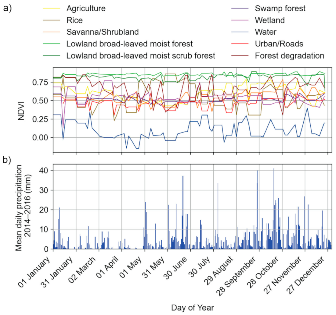
2.4. Training and Validation Data

One of the goals of this study was to develop a single algorithm that can be applied across the Landsat record. Therefore, we trained the algorithm on Landsat 8 data for the most recent period (2014–2016) of this study and then applied the trained algorithm to the other Landsat sensors in the earlier periods. Separate validation datasets were used for each period to assess the transferability of the algorithm across sensors and time.

First, we created polygons to select training data for the 2014–2016 period based on GPS data collected on the ground and expert knowledge of the study area (the authors have over 60 years of combined experience in the study area beginning in 1992). The polygons were created in Google Earth Engine based on the ground information and visual interpretation of the Landsat seasonal composites for 2014–2016, individual Landsat images from each year of the composite period, and Google Earth satellite data. While the expert knowledge of the area allowed us to select training and validation data confidently for 1999–2001 and 2014–2016, the 1984–1987 polygons relied on visual interpretation of the Landsat data and historical context. The seasonal composites were particularly useful for determining wetlands, and the individual images from each year were used to find areas of deforestation that occurred during the composite period. We randomly sampled 450 pixels per class contained within the training polygons using the stratified random sampling method in Google Earth Engine.

Next, we repeated the process to create polygons to select validation pixels for each class that did not overlap with the training polygons. A randomly sampled set of 450 pixels per class were selected from these validation polygons to create an independent validation dataset. We use an independent set of an equal number of samples for training and validation data to fairly assess the performance of the algorithm across space as well as time. For the 1984–1987 and 1999–2001 periods, we repeated the process of creating polygons for each class and randomly sampled 450 pixels per class to use for validation.

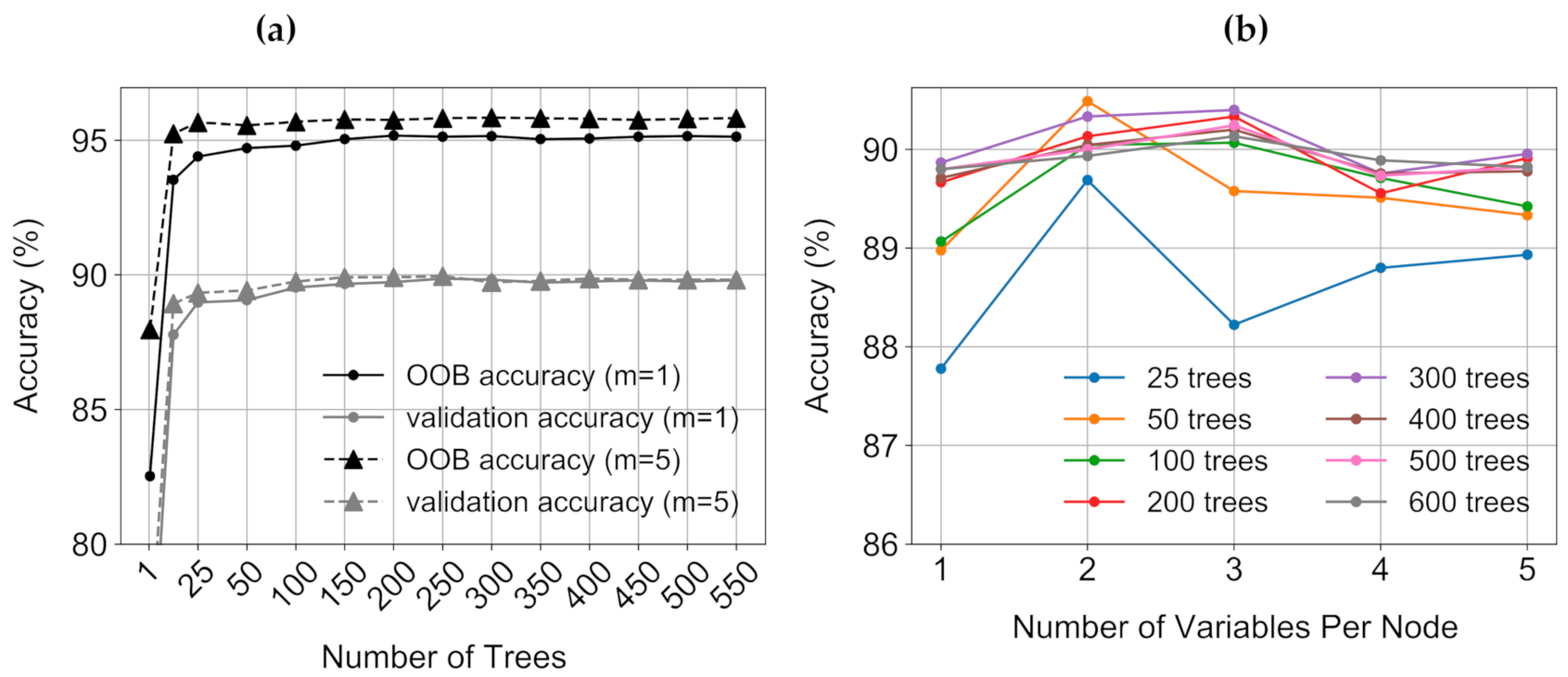
2.5. Optimizing Random Forest

Random forest is considered to be a robust algorithm with few parameters to optimize, and the effects of parameters are insignificant at high levels of trees [25,27]. The main parameters that affect the algorithm’s accuracy are the number of regression trees created (t) and the number of variables used at each node in the tree (m). To achieve the highest accuracy algorithm to apply across periods, we optimized t and m by testing a range of values for each variable and calculating the out-of-bag error (OOB), the training accuracy, and the overall validation accuracy for each combination of parameters for the training period of 2014–2016. The number of training and validation samples were held at 450 pixels per class for all algorithm combinations, and 30% of the training data in each run were withheld for calculation of the OOB error and training accuracy. Previous studies have shown that at high values of t, there is little to no increase in accuracy and that the highest accuracies are achieved with low values of m (Rodríguez-Galiano et al. 2012). Therefore, we tested every combination of t = 1, 25, 50, 100, 150, 200, 250, 300, 350, 400, 450, 500, 550, 600 and m = 1, 2, 3, 4, 5, resulting in 70 total RF algorithms to compare.

The optimal parameter combination was determined using a sensitivity analysis based on the OOB error, training, and validation accuracies calculated from all combinations of t and m. The optimal algorithm was determined as the one that achieved the highest training and validation accuracies while maintaining the lowest OOB error. We applied the optimized algorithm to the earlier periods, assessing accuracy with the validation data sets for each period to evaluate how well the single algorithm performs through time. In addition to overall accuracy, confusion matrices revealed which classes were most misclassified by the algorithm. We then combined classes that were highly confused in the results and reassessed the accuracy, resulting in eight final LULC classes. We combined the lowland broad-leaved moist forest and lowland broad-leaved moist scrub forest classes, as they are similar forest types, and the species differences are not important for assessing forest loss in this study. Additionally, the agriculture and forest degradation classes were combined, as the deforestation in the study area is almost entirely for agriculture, and so can be considered agriculture in this study. These final eight classes were used to calculate the area and percent of each LULC in each time period and the percent of change between each of the three maps.

3. Results

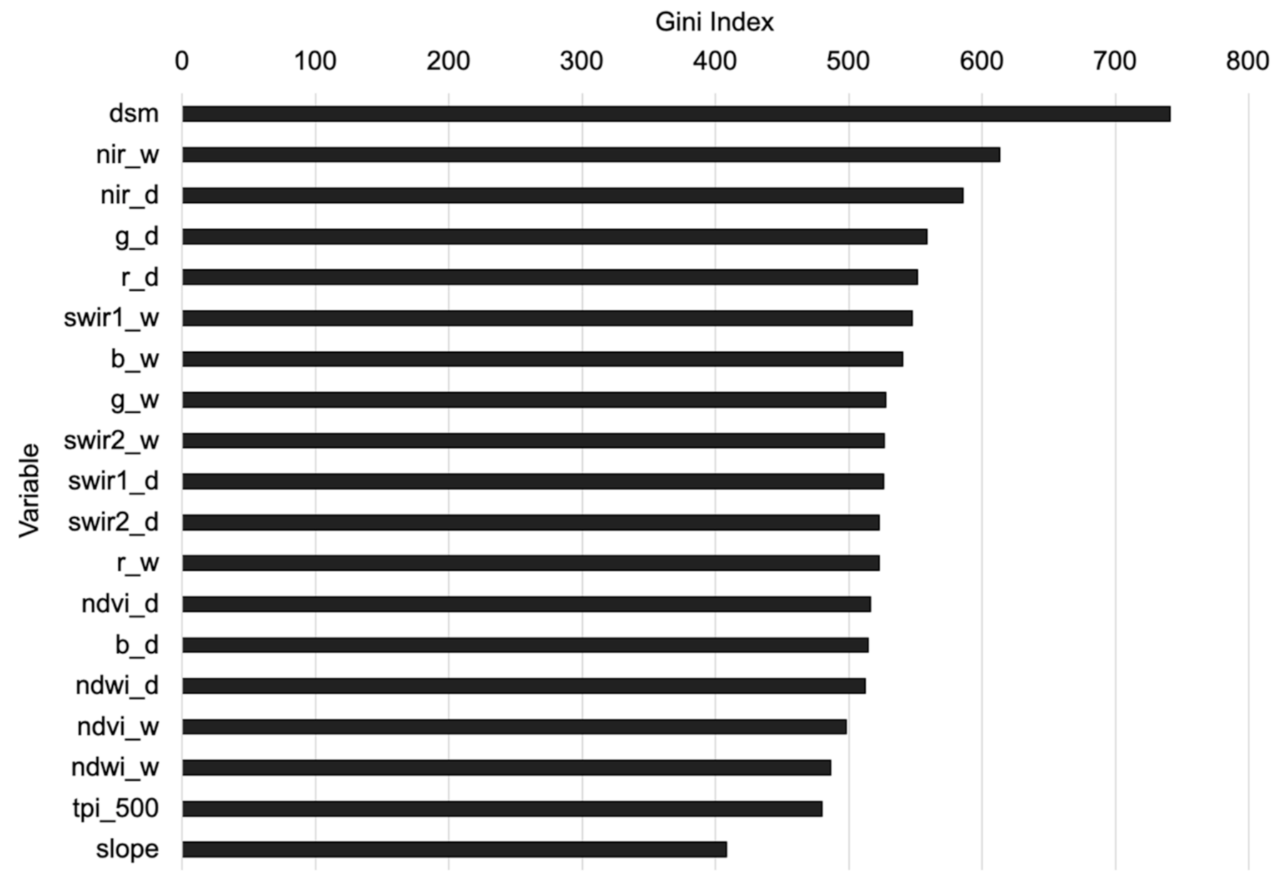
3.1. Algorithm Selection and Variable Importance

Increasing the number of trees in the RF increased both OOB and validation accuracies sharply up to 25 trees, while gains in accuracy diminished above 100 trees. At all values of m, both the validation accuracy and OOB accuracy reached a maximum at around 300 trees (Figure 3). At t = 25 and 50, the highest accuracy was achieved with m = 2, but at all values of t ≥ 100, the accuracy was highest at m = 3 (Figure 3). Therefore, the final algorithm selected for land cover mapping had t = 300 and m = 3, with 450 pixels per class used for training with 10 land cover classes.

The RF algorithm used the Gini index to assess the relative amount that each variable contributed to the difference between classes in the classification [54]. Higher values of the Gini index represent higher importance in the final classification accuracy and a larger contribution to maximizing the difference between classes. Since ecosystems are strongly correlated with topography in this area, it is not surprising that the elevation from the ALOS-2 DSM was the most important variable in the classification (Figure 4). In addition, the majority of the agriculture occurs in the flat areas of the coastal plain. The next most important variables were the wet season NIR and the dry season NIR composites. The NIR wavelength is highly sensitive to water content as well as chlorophyll and is used in the calculation of both NDVI and NDWI, and the seasonal differences reflected plant phenology and seasonal inundation. The least important variable was slope gradient, calculated from the ALOS-2 DSM. While slope likely does influence LULC distributions, most of the study area occupies the relatively flat coastal plain, so there was little slope variation in the analysis. Moreover, where there is a high gradient in steeply faulted and karst collapse escarpments, and Landsat and ALOS-2 resolutions may have been too low to capture some of these changes.

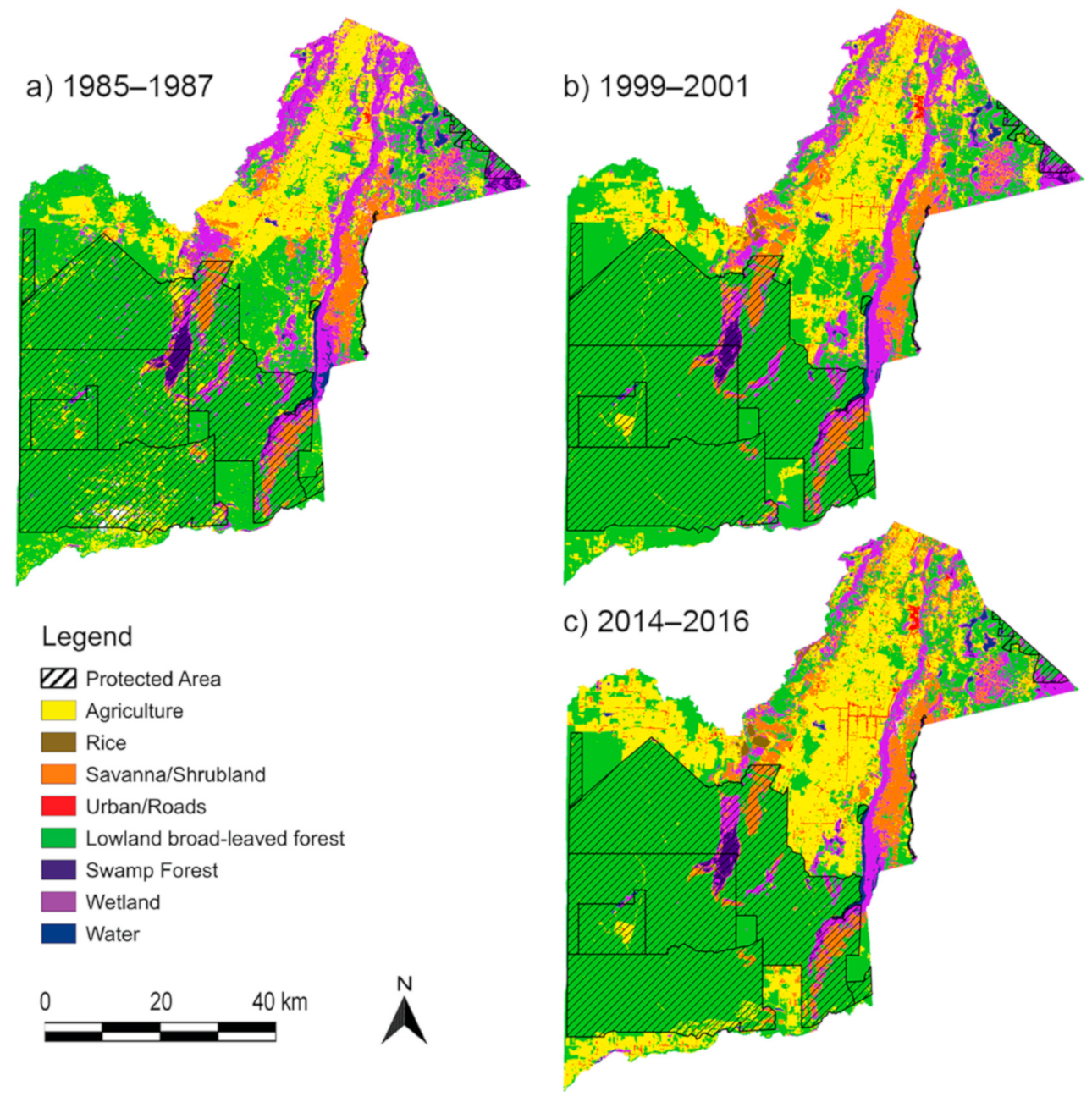
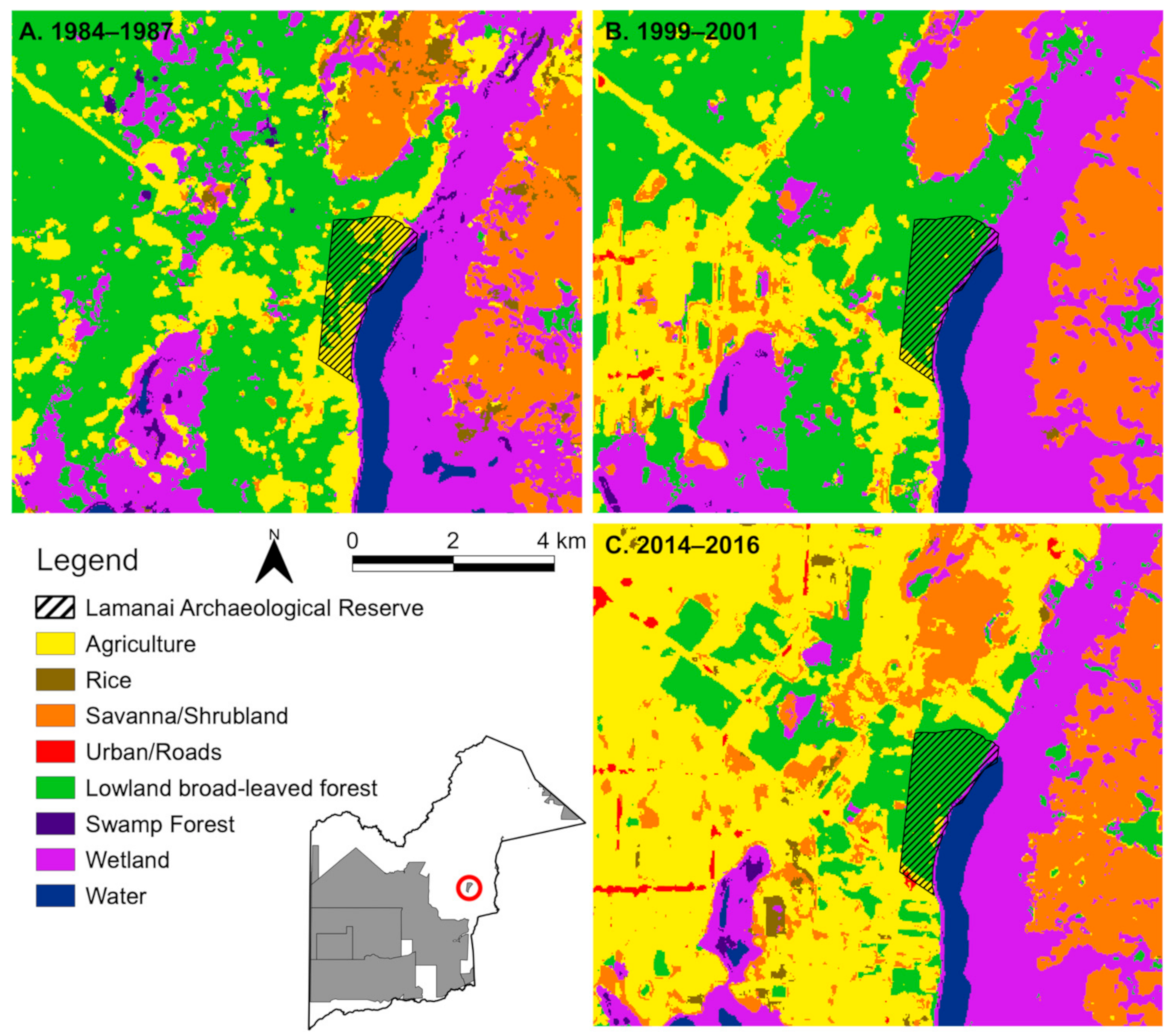
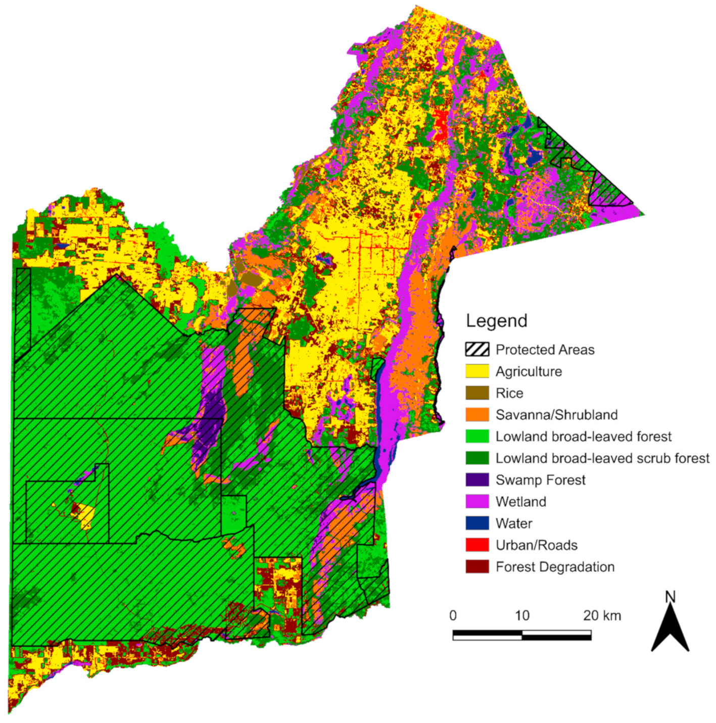
3.2. 2014–2016 Land-Use Land Cover Classification

The final model with t = 300 and m = 3 achieved an overall accuracy of 90.2% across the 10 LULC classes for the 2014–2016 period (

Table 4. Classification producer accuracy (PA) and user accuracy (UA) of each class for the 3 periods with 10 classes and 8 classes (scrub forest combined with forest and forest degradation combined with agriculture).

		2014–2016		1999–2001		1984–1987
Class	No. Classes	PA (%)	UA (%)	PA (%)	UA (%)	PA (%)	UA (%)
Agriculture	10 classes	89.78	70.88	86.22	74.90	82.00	48.55
	8 classes	94.22	80.30	83.56	88.68	89.33	61.94
Rice	10 classes	84.67	98.96	77.56	96.94	NA	0.00
	8 classes	85.11	98.97	77.56	97.21	NA	0.00
Savanna	10 classes	97.56	89.78	99.56	81.45	94.67	84.36
	8 classes	97.56	92.23	99.56	89.07	94.67	85.37
Urban	10 classes	82.67	97.64	87.33	98.25	40.67	97.34
	8 classes	82.67	97.89	87.33	100.00	40.67	97.86
Forest	10 classes	95.33	90.51	6.00	100.00	1.11	100.00
	8 classes	99.33	96.13	97.78	94.02	93.11	95.88
Swamp forest	10 classes	96.67	95.81	99.56	97.39	98.22	92.08
	8 classes	96.67	95.81	99.56	97.39	98.22	92.08
Wetland	10 classes	90.22	87.50	95.33	80.49	85.33	82.05
	8 classes	90.22	88.84	95.33	81.25	85.33	92.53
Water	10 classes	99.33	98.68	100.00	96.77	99.11	94.09
	8 classes	99.33	98.68	100.00	96.77	99.11	94.09
Scrub forest	10 classes	91.78	91.37	96.67	41.91	83.56	41.23
	8 classes	-	-	-	-	-	-
Forest degradation	10 classes	76.00	90.48	24.22	73.15	37.11	67.61
	8 classes	-	-	-	-	-	-
Overall accuracy (OA %)	10 classes	90.2%		79.4%		69.0%
	8 classes	92.6%		93.6%		85.7%

). The classes with the lowest accuracies were forest degradation and agriculture, which were most confused with each other. The confusion of these two classes makes sense because the deforestation in this area is almost entirely driven by different types of agriculture in this period, and so the forest degradation ultimately becomes agriculture. The algorithm mapped rice well (producer accuracy = 84.67%, user accuracy = 98.96%), but understandably sometimes confused rice for wetland or vice versa. The three key distinctions between the rice and wetland classes were that the rice fields are flooded during the dry season with irrigation, harvested and drained, and often burned before the wet season. Alternatively, many wetlands flood with the wet season (though some are perennial) and dry with the dry season. Using the seasonal data allows the algorithm to not only identify seasonal wetlands but distinguish seasonal wetlands from irrigated rice agriculture. The urban class was also not always distinguishable from the savanna and agriculture classes, likely because there is little area that is actually densely built environment, and buildings are often interspersed between large yards, fields, and gardens. These low-density towns and narrow limestone roads were difficult to identify in the 30 m spatial resolution of Landsat pixels.

Algorithm performance decreased when applied to the earlier years with previous Landsat sensors (Table 4). Even after normalizing the sensor data to Landsat 8 (31), there likely remained differences in the spectral data from each sensor. It is important to note that the previous periods have far fewer images available (Table 1), which affected the median composite values and left some pixels without any available data. With Landsat 8 data from 2014–2016, the RF was able to distinguish between the two different types of broad-leaved forests in the study area, but when applied to past sensors, these forest types were indistinguishable. While species compositions may differ, it was appropriate to combine these two forest types into a single tropical forest class to meet the goal of quantifying forest loss. Most of the forest degradation class that could be mapped reliably with the recent Landsat 8 data (PA = 76%; UA = 90.48%) was fairly indistinguishable from agriculture in the earlier periods (PA = 24.22%, UA = 73.15% for 1999–2001; PA = 37.11%, UA = 67.61% for 1984–1987). In Orange Walk, most of the deforestation is for conversion to agriculture, usually where agriculture meets the forest edge (Figure 7). Hence, combining these two classes was again appropriate for this study. In the earliest period, 1984–1987, some of the agriculture (some originally classified as forest degradation) was likely other types of rotational agriculture (milpa), illicit growing plots, and selective logging, none of which are nearly as prevalent in the two more recent periods. Therefore, for assessing land-use and land-cover change across time, we combined these two pairs of classes to create the eight final classes (Table 1).

With the classification results combined into eight classes, the algorithm performed well in the earlier periods, and the overall accuracy increased for every period (Table 4). When applied to the 1999–2001 data, the overall accuracy increased by 1%, to 93.6%, and when applied to 1984–1987 data, the overall accuracy was lower, but still useful at 85.7%. The earliest period had less than 33% of the number of Landsat images available as the later periods did. Thus, it was likely that the lower frequency of observations in the earliest classification affected its composite values and contributed to its higher error rate.

The land-cover and land-use maps revealed changes in land-use patterns and the losses of tropical forest and wetlands over recent decades (Figure 5). The area classified as agriculture decreased from 1984–1987 to 1999–2001 by nearly 100 km², but wetlands (including wetland and swamp forest) decreased by 115.2 km² (Table 7). From 1999–2001 to 2014–2016, the agriculture class increased by nearly 350 km². The early decrease in agriculture can be attributed to multiple factors. First, the 1984–1987 period was before the establishment of the protected areas that now occupy much of the district and when there were active logging and milpa agriculture in these now protected forests [55]. After the establishment of public and private protected areas during the late 1980s and 1990s, these areas showed reforestation, but zones outside of the protected areas experienced a drastic increase in intensive agriculture (Figure 5).

The largest increase in the area of any class between the 1999–2001 and 2014–2016 periods was agriculture, which gained 347.68 km², representing an increase of 43.6% (

Table 5. Transition matrix of lands cover classes between maps for 1984–1987 and 1999–2001 in km².

	Agriculture	Rice	Savanna/ Shrubland	Urban/ Roads	Lowland Forest	Swamp Forest	Wetland	Water
Agriculture	485.88	3.46	78.84	16.09	275.87	0.01	37.87	0.00
Rice	3.88	1.24	8.94	0.36	0.09	0.06	7.69	0.01
Savanna/shrubland	33.49	0.86	237.16	1.01	4.61	0.02	33.22	0.00
Urban/roads	4.13	0.11	0.59	6.79	0.03	0.00	0.03	0.00
Lowland forest	222.53	1.26	21.11	1.51	2415.10	0.06	16.60	0.00
Swamp forest	0.68	0.23	0.54	0.00	7.90	34.29	20.91	0.23
Wetland	46.80	8.13	54.91	0.75	100.18	5.37	390.17	1.24
Water	0.02	0.01	0.04	0.00	0.29	0.64	9.94	29.02

,

Table 6. Transition matrix of lands cover classes between maps for 1999–2001 and 2014–2016 in km².

	Agriculture	Rice	Savanna/ Shrubland	Urban/ Roads	Lowland Forest	Swamp Forest	Wetland	Water
Agriculture	640.98	4.34	55.11	17.91	72.71	0.13	6.50	0.65
Rice	4.86	5.90	2.66	0.36	0.20	0.06	1.45	0.01
Savanna/shrubland	80.51	5.53	262.13	2.19	11.41	0.13	41.00	0.03
Urban/roads	8.01	0.21	0.16	18.10	0.02	0.00	0.02	0.00
Lowland forest	371.15	3.49	22.75	3.02	2408.51	0.18	5.74	0.81
Swamp forest	0.03	0.06	0.02	0.00	1.48	26.82	11.86	0.27
Wetland	39.98	8.02	43.86	0.24	110.72	8.57	302.39	3.25
Water	0.00	0.00	0.00	0.00	0.00	0.22	2.18	28.23

and

Table 7. Area of each land cover class during each time period.

Class	1984–1987 (km2)	1999–2001 (km2)	2014–2016 (km2)
Agriculture	898.00	798.09	1145.77
Rice	22.21	15.51	27.51
Savanna/scrubland	310.47	403.10	386.70
Urban/roads	11.72	26.57	41.80
Lowland broad-leaved moist forest	2677.52	2815.55	2605.08
Swamp forest	64.85	40.65	36.27
Wetland	607.73	516.71	371.11
Water	39.90	30.56	33.10
Population Orange Walk 1985 est, 2000, 2016 est	26,776	40,301	50,208

). The classes that lost the most area were lowland broad-leaved forest and wetlands, losing 210.47 and 145.6 km², respectively. The urban/road class only increased by 15.22 km², but given the low amount of that class in the study area, this increase represents 57.3% growth for that class during this time period. We also know from yearly field research in this area that road paving and accessibility has increased significantly over this time.

Another factor was the doubling of the population in Orange Walk District. We used a simple mean between 1980 and 1990 censuses for the 1985 estimate, the census figure for 2000, and the census estimate for 2016 for these baseline population growth numbers [56]. We lacked rural numbers where land-use changes were taking place, but the District population provided a general trend, and it grew by 33.6% from 1985 to 2000 and by 19.7% from 2001 to 2016. Population growth was greatest in the first period from 1985–2000, but agriculture increased by a much higher percent from 2000 to 2015 (

Table 8. Area change in each class compared to prior period (~15 years) in km² with the percent change in parentheses.

Class	1984–1987 to 1999–2001	1999–2001 to 2014–2016
Agriculture	−99.92 (−11.1%)	+347.68 (43.6%)
Rice	−6.70 (−30.1%)	+12.00 (77.4%)
Savanna/scrubland	+92.63 (29.9%)	−16.40 (−4.1%)
Urban/roads	+14.86 (126.8%)	+15.22 (57.3%)
Lowland broad-leaved moist forest	+138.03 (5.2%)	−210.47 (−7.5%)
Swamp forest	−24.21 (−37.3%)	−4.38 (−10.8%)
Wetland	−91.01 (−15.0%)	−145.60 (−28.2%)
Water	−9.34 (−23.4%)	+2.53 (8.3%)
Population	+13,525 (33.6%)	+9907 (19.7%)

).

4. Discussion

By using data harmonization, multitemporal data, and machine learning, we were able to achieve our goals of developing a time-generalized land-cover classifier and quantifying land-use and land-cover change in Orange Walk, Belize with the Landsat archive. The approach used multi-season data to distinguish land-use and land-cover types and multiyear data to acquire nearly complete coverage and derive median values that were more comparable through time after applying sensor harmonization coefficients [33]. The results of the classifications revealed a rapid loss of tropical forest and two types of wetlands due to agricultural expansion since 2000. These losses occurred during a time of population growth in Orange Walk, Belize, but forest and wetland loss was far greater than the increase in population since 2000 relative to the higher population growth from 1984–2000. Moreover, the role of conservation in landscape patterns and the protection of natural and cultural resources in Orange Walk was reflected in the distributions of land-use land-cover through time. In 1984–1987, before the establishment of protected areas, small clearings were prolific throughout the forests. By 1999–2001, the now protected forests grew back, but continuous clear-cutting for mechanized agriculture had begun to increase outside of the protected areas, continuing to expand rapidly through 2016.

We achieved our first goal by optimizing an RF algorithm trained with Landsat 8 data and successfully classifying LULC with harmonized Landsat 4, 5, and 7 data. After initially running a sensitivity analysis of the RF parameters to achieve high accuracy (>90%) with 10 classes in the Landsat 8 data, we found that combining classes to 8 more general classes resulted in much higher accuracy when applying the algorithm to the earlier data. The combination of the two pairs of classes, however, did not affect the interpretation of our results because the distinction between these classes was subtle and not important for the application of this study. Multiple factors likely contributed to the decrease in accuracy of the algorithm applied to the past time periods. First, even after harmonizing the Landsat 4, 5, and 7 data, the spectral resolutions and consistency across sensors did not perfectly match [33]. In the experiments training with and classifying the Landsat 8 data, the algorithm was able to distinguish between the two forest types in the original 10-category classification scheme. The algorithm could not distinguish these forest types from each other when applied to the earlier datasets, however, likely because the NDVI phenological signatures of the two forest types were similar (Figure 2). Additionally, fewer Landsat scenes were available for 1984–1987 and 1999–2001 than for 2014–2016 (Table 2). As a result, the seasonal median composite values in the earliest data were comprised of far fewer samples and will likely produce median values that differ from the Landsat 8 training samples due to sample size. Previous studies demonstrated that using monthly median composites across multiple years improved the application of an RF algorithm across time [46]. Here, we demonstrated that even just two seasonal median composites created from multiple years of data could produce a time-generalized classifier for general LULC categories.

After using the optimized algorithm to map LULC during three time periods, we were able to quantify these changes in our study area. While Orange Walk had forest regrowth between 1984 and 1987 and 1999–2001 (~15 years) due to the establishment of protected areas, there was a significant loss of forest and wetlands, 210.47 km² and 145.6 km², respectively, from 1999–2001 to 2014–2016 (~15 years). During this more recent period, the agricultural area increased by 347.68 km². The total loss of forest and wetland classes closely matches the gain in the agriculture class during this most recent period. Interestingly, the population grew much more in Orange Walk during the 15 years between the 1984–1987 and 1999–2001 periods (13,525 people) than it did between the 1999–2001 and 2014–2016 periods (9,907 people), while the deforestation was much greater during this later period. We do not have enough data to directly infer a relationship between population growth and deforestation, but studies in the global tropics have observed that shifts to large commercial agriculture from small landowners change the relationship between population and forest cover [5,57].

The deforestation that occurred in 1984–1987 in the RBCMA was classified as agriculture in this study, but there were other contributions to the observed deforestation that differed from the industrial agricultural, driving most of the long-term deforestation. In the earliest period, the agriculture area within what is now the RBCMA also consisted of milpa agriculture and possibly illicit agriculture and logging. In the Toledo district in southern Belize, Emch et al. [58] estimated that ~360 km² of forest were lost between 1975 and 1999 and that the primary driver was increased milpa agriculture due to a 259% increase in the population [58]. The rapid expansion of industrial agriculture in recent decades has occurred in the Mennonite communities of Northwest Belize. In Campeche, Mexico, Mennonite industrial farming lands had ~4 times higher rate of deforestation than on other private property [59]. Land tenure and expansion of the agro-industrial production model were considered to be the major drivers of forest loss in the central Yucatan; communal property experienced significantly less forest loss. In other parts of Central America, including in similar forests in adjacent Guatemala, narcotics production and trafficking can drive deforestation as well [60].

There are no current studies that estimate LULC change for the entire Landsat record for Orange Walk, but other studies have estimated deforestation rates for other parts of Belize or Belize as a whole. A study of tropical forest loss using Landsat data estimated that all of Belize lost 80 km² per year of the forest, defined as >30% tree cover, between 1990 and 2000 and 70 km² per year from 2000–2010 [1]. Voight et al. [24] estimated that in the Maya Golden Landscape in southern Belize, 20.9 km² of mature forest were cleared from 2014–2016.

Another key finding is the role of conservation areas in reforestation and forest maintenance. The Rio Bravo Conservation and Management Area (RBCMA) (Figure 1) showed both reforestation from its founding in 1988 as well as forest maintenance in this area. Figure 5 shows that areas that were to become the RBCMA had ~56 km² of deforestation before its establishment (Figure 5a), but ~42 km² were reforested by ~2000 (Figure 5b) and another ~20 km² increase in the forest through ~2015 (Figure 5c). For example, the area of the RBCMA around the ancient Maya site of Gran Cacao, even though it is difficult to access today, had a few square kilometers of deforested area, but these became reforested by 2000 and are currently closed-canopy forest (Figure 5). The southern part of Orange Walk in what is now the privately managed Yalbac Ranch experienced similar deforestation in the earliest years with forest regrowth and maintenance since (Figure 5).

The protected Archaeological Preserve of the important ancient Maya city of Lamanai remained forested, but deforestation on its west side has occurred up the small park’s boundary. Additionally, the wetlands to the west have decreased in an area with drainage and conversion to agriculture. Deforestation there has also taken place over numerous ancient Maya mounds on private property in well-drained uplands, but not so in wetlands and lower-lying savannas to Lamanai’s east. Once surrounded by tropical forest, the Lamanai Archaeological Reserve now stands as an island of forest in an expanse of agricultural fields (Figure 6).

The changes in land-use and land-cover patterns revealed by these maps demonstrate the importance of protected land for the conservation of both natural and cultural resources. In the most recent map, most of the forest that is not in protected areas has already been deforested (Figure 7). Our results estimate that about 627 km² of forest remain unprotected while about 1978 km² (76%) of forest in Orange Walk is in protected areas today. With little area left for agriculture to expand into, the protected areas remain essential for conserving the biodiversity and habitat of these forests. The protected area of the RBCMA is particularly important for jaguar and peccary conservation, and efforts should aim to increase the habitat connectivity and corridors between the protected areas of Belize [11]. While previous studies in the region and international conservation efforts mainly focus on forest ecosystems, this study suggests that wetland ecosystems should be equally considered in conservation efforts. While the establishment of protected areas helped forest regrowth between 1984 and 1987 and 1999–2001, wetlands and swamp forests still declined by 115 km². While both forests and wetlands continue to be rapidly lost, conservation efforts should include wetlands, and not just forests, in their efforts to preserve natural resources.

It is important to note, however, that the increase in agricultural production is important for developing food security and economic commodities, as well as local economies. Further, land-use and conservation planning should aim to balance the urgency of protecting cultural and natural resources with the economic and social needs of the population.

5. Conclusions

Land-use land-cover change in the tropics can be accurately mapped across the Landsat archive with a random forest classifier by including multi-season and multiyear composites. While many studies rely on a single sensor or single date imagery, the multitemporal machine learning approach in this study allowed for the distinction of more land-use and land-cover types and the ability to use the entire Landsat archive. This novel approach revealed that tropical forests and wetlands are under threat from rapidly expanding industrial agriculture in Northwest Belize and that the remaining tracts of these valuable ecosystems are largely within protected areas. Early deforestation (1984–1987) was likely driven by a combination of milpa agriculture, illicit agriculture, and selective logging, as well as some industrial agriculture. The establishment of the RBCMA in 1988 and the subsequent protected areas allowed for forest regrowth in the 1990s, though wetland losses were high at 15%. Between 1999 and 2001 and 2014–2016, however, industrial agriculture rapidly spread across all areas that were not protected with heavy losses of tropical forest (7.5%) and the continued loss of wetlands (28.2%). As a result, the protected areas in Orange Walk are critical to preserving the remaining forests and wetlands in the district. These threatened ecosystems provide essential ecosystem services and habitat for maintaining biodiversity, connectivity of wildlife corridors, and threatened species. The protected areas also protect the cultural heritage that is threatened with land-use and land-cover change, such as in our case study of the ancient Maya site of Lamanai, which is now an island of preserved forest. Agriculture provides an important means of food security and economic development for Belize, but its rapid increase has occurred across biodiverse ecosystems and millennia of ancient Maya structures. Combining new advances in computing and machine learning with the growing length of the satellite record allows us to provide robust estimates of these threatened natural and cultural resources and inform conservation and land management policies and decision-making.

References

1. Kim, D.-H.; Sexton, J.O.; Townshend, J.R. Accelerated deforestation in the humid tropics from the 1990s to the 2000s. Geophys. Res. Lett. 2015, 42, 3495–3501. [Google Scholar] [CrossRef] [PubMed]
2. Myers, N. Threatened biotas: “Hot spots” in tropical forests. Environmentalist 1988, 8, 187–208. [Google Scholar] [CrossRef] [PubMed]
3. Geist, H.J.; Lambin, E.F. Proximate Causes and Underlying Driving Forces of Tropical Deforestation. Bioscience 2002, 52, 143. [Google Scholar] [CrossRef]
4. Lambin, E.F.; Turner, B.L.; Geist, H.J.; Agbola, S.B.; Angelsen, A.; Bruce, J.W.; Coomes, O. The causes of land-use and land-cover change: Moving beyond the myths. Glob. Environ. Chang. 2001, 11, 261–269. [Google Scholar] [CrossRef]
5. Rudel, T.K.; Defries, R.; Asner, G.P.; Laurance, W.F. Changing Drivers of Deforestation and New Opportunities for Conservation. Conserv. Biol. 2009, 23, 1396–1405. [Google Scholar] [CrossRef] [PubMed]
6. Foley, J.A.; DeFries, R.; Asner, G.P.; Barford, C.; Bonan, G.; Carpenter, S.R.; Chapin, F.S.; Coe, M.T.; Daily, G.; Gibbs, H.; et al. Global consequences of land use. Science 2005, 309, 570–574. [Google Scholar] [CrossRef] [Green Version]
7. Lambin, E.F.; Meyfroidt, P. Global land use change, economic globalization, and the looming land scarcity. Proc. Natl. Acad. Sci. USA 2011, 108, 3465–3472. [Google Scholar] [CrossRef] [Green Version]
8. Song, X.P.; Hansen, M.C.; Stehman, S.V.; Potapov, P.V.; Tyukavina, A.; Vermote, E.F.; Townshend, J.R. Global land change from 1982 to 2016. Nature 2018, 560, 639–643. [Google Scholar] [CrossRef]
9. Chaudhary, A.; Mooers, A.O. Terrestrial vertebrate biodiversity loss under future global land use change scenarios. Sustainability 2018, 10, 2764. [Google Scholar] [CrossRef] [Green Version]
10. Young, C. Belize’s Ecosystems: Threats and Challenges to Conservation in Belize. Trop. Conserv. Sci. 2008, 1, 18–33. [Google Scholar] [CrossRef] [Green Version]
11. Hofman, M.P.G.; Hayward, M.W.; Kelly, M.J.; Balkenhol, N. Enhancing conservation network design with graph-theory and a measure of protected area effectiveness: Refining wildlife corridors in Belize, Central America. Landsc. Urban Plan. 2018, 178, 51–59. [Google Scholar] [CrossRef]
12. Beach, T.; Luzzadder-Beach, S.; Krause, S.; Guderjan, T.; Valdez, F.; Fernandez-Diaz, J.C.; Eshleman, S.; Doyle, C. Ancient Maya wetland fields revealed under tropical forest canopy from laser scanning and multiproxy evidence. Proc. Natl. Acad. Sci. USA 2019, 116, 21469–21477. [Google Scholar] [CrossRef] [PubMed] [Green Version]
13. Canuto, M.A.; Estrada-Belli, F.; Garrison, T.G.; Houston, S.D.; Acuña, M.J.; Kovác, M.; Marken, D.; Nondédéo, P.; Auld-Thomas, L.; Castanet, C.; et al. Ancient lowland Maya complexity as revealed by airborne laser scanning of northern Guatemala. Science 2018, 361, 6409. [Google Scholar] [CrossRef] [PubMed] [Green Version]
14. Chase, A.F.; Chase, D.Z.; Awe, J.J.; Weishampel, J.F.; Iannone, G.; Moyes, H.; Yaeger, J.; Brown, M.K. The use of LiDAR in understanding the Ancient Maya Landscape. Caracol and Western Belize. Adv. Archaeol. Pract. A J. Soc. Am. Archaeol. 2014, 2, 208–221. [Google Scholar] [CrossRef] [Green Version]
15. Cherrington, E.A.; Ek, E.; Cho, P.; Howell, B.F.; Hernandez, B.E.; Anderson, E.R.; Flores, A.; Garcia, B.; Sempris, E.; Irwin, D. Forest Cover and Deforestation in Belize: 1980–2010. Serv. Tech. Rep. 2012. Available online: http://www.servir.net/servir_bz_forest_cover_1980-2010.pdf (accessed on 25 August 2020).
16. Chicas, S.D.; Omine, K.; Ford, J.B.; Sugimura, K.; Yoshida, K. Using spatial metrics and surveys for the assessment of trans-boundary deforestation in protected areas of the Maya Mountain Massif: Belize-Guatemala border. J. Environ. Manag. 2017, 187, 320–329. [Google Scholar] [CrossRef]
17. Wyman, M.S.; Stein, T.V. Modeling social and land-use/land-cover change data to assess drivers of smallholder deforestation in Belize. Appl. Geogr. 2010, 30, 329–342. [Google Scholar] [CrossRef]
18. Beach, T.; Luzzadder-Beach, S.; Cook, D.; Dunning, N.; Kennett, D.J.; Krause, S.; Terry, R.; Trein, D.; Valdez, F. Ancient Maya impacts on the Earth’s surface: An Early Anthropocene analog? Quat. Sci. Rev. 2015, 124, 1–30. [Google Scholar] [CrossRef] [Green Version]
19. Camille, M.A. The Effects of Timber Haulage Improvements on Mahogany Extraction in Belize: An Historical Geography. Yearbook Conf. Latin Am. Geogr. 2000, 26, 103–115. [Google Scholar]
20. Bernsten, R.H.; Herdt, R.W. Towards an Understanding of Milpa Agriculture: The Belize Case. J. Dev. Areas 1977, 11, 373–392. [Google Scholar]
21. Levasseur, V.; Olivier, A. The farming system and traditional agroforestry systems in the Maya community of San Jose, Belize. Agrofor. Syst. 2000, 49, 275–288. [Google Scholar] [CrossRef]
22. Steinberg, M.K. Political ecology and cultural change: Impacts on swidden-fallow agroforestry practices among the mopan maya in southern Belize. Prof. Geogr. 1998, 50, 407–417. [Google Scholar] [CrossRef]
23. Chomitz, K.M.; Gray, D.A. Roads, Land Use, and Deforestation: A Spatial Model Applied to Belize. World Bank Econ. Rev. 1996, 10, 487–512. [Google Scholar] [CrossRef] [Green Version]
24. Voight, C.; Hernandez-Aguilar, K.; Garcia, C.; Gutierrez, S. Predictive modeling of future forest cover change patterns in southern Belize. Remote Sens. 2019, 11, 823. [Google Scholar] [CrossRef] [Green Version]
25. Talukdar, S.; Singha, P.; Mahato, S.; Pal, S.; Liou, Y.A.; Rahman, A. Land-use land-cover classification by machine learning classifiers for satellite observations-A review. Remote Sens. 2020, 12, 1135. [Google Scholar] [CrossRef] [Green Version]
26. Ge, Y.; Hu, S.; Ren, Z.; Jia, Y.; Wang, J.; Liu, M.; Zhang, D.; Zhao, W.; Luo, Y.; Fu, Y.; et al. Mapping annual land use changes in China’s poverty-stricken areas from 2013 to 2018. Remote Sens. Environ. 2019, 232, 111285. [Google Scholar] [CrossRef]
27. Rodríguez-Galiano, V.F.; Ghimire, B.; Rogan, J.; Chica-Olmo, M.; Rigol-Sanchez, J.P. An assessment of the effectiveness of a random forest classifier for land-cover classification. ISPRS J Photogramm. Remote Sens. 2012, 67, 93–104. [Google Scholar]
28. Denisko, D.; Hoffman, M.M. Classification and interaction in random forests. Proc. Natl. Acad. Sci. USA 2018, 115, 1690–1692. [Google Scholar] [CrossRef] [Green Version]
29. Grinand, C.; Rakotomalala, F.; Gond, V.; Vaudry, R.; Bernoux, M.; Vieilledent, G. Estimating deforestation in tropical humid and dry forests in Madagascar from 2000 to 2010 using multi-date Landsat satellite images and the random forests classifier. Remote Sens. Environ. 2013, 139, 68–80. [Google Scholar] [CrossRef]
30. Gorelick, N.; Hancher, M.; Dixon, M.; Ilyushchenko, S.; Thau, D.; Moore, R. Google Earth Engine: Planetary-scale geospatial analysis for everyone. Remote Sens. Environ. 2017, 202, 18–27. [Google Scholar] [CrossRef]
31. Lee, J.; Cardille, J.A. Agricultural Expansion in Mato Grosso from 1986–2000: A Bayesian Time Series Approach to Tracking Past Land Cover Change. Remote Sens. 2020, 12, 688. [Google Scholar] [CrossRef] [Green Version]
32. Oliphant, A.J.; Thenkabail, P.S.; Teluguntla, P.; Xiong, J.; Gumma, M.K.; Congalton, R.G.; Yadav, K. Mapping cropland extent of Southeast and Northeast Asia using multi-year time-series Landsat 30-m data using a random forest classifier on the Google Earth Engine Cloud. Int. J. Appl. Earth Obs. Geoinf. 2019, 81, 110–124. [Google Scholar] [CrossRef]
33. Roy, D.P.; Kovalskyy, V.; Zhang, H.K.; Vermote, E.F.; Yan, L.; Kumar, S.S.; Egorov, A. Characterization of Landsat-7 to Landsat-8 reflective wavelength and normalized difference vegetation index continuity. Remote Sens. Environ. 2016, 185, 57–70. [Google Scholar] [CrossRef] [Green Version]
34. Marshall, J.S. The Geomorphology and Physiographic Provinces of Central America. Cent. Am. Geol. Resour. Hazards 2007, 1, 75–121. [Google Scholar]
35. Beach, T.; Luzzadder-Beach, S.; Dunning, N.; Jones, J.; Lohse, J.; Guderjan, T.; Bozarth, S.; Millspaugh, S.; Bhattacharya, T. A review of human and natural changes in Maya Lowland wetlands over the Holocene. Quat. Sci. Rev. 2009, 28, 1710–1724. [Google Scholar] [CrossRef]
36. Meerman, J.C.; Sabido, W. Central American Ecosystems Map: Belize. Belize City Programme Belize 2001, 2, 1–88. [Google Scholar]
37. Brokaw, N.; Mallory, E.P. Vegetation of The Rio Bravo Conservation and Management Area, Belize. Mass. Manomet Bird Obs. 1993, 1, 1–53. [Google Scholar]
38. Brewer, S.W.; Webb, M.A.H. A seasonal evergreen forest in Belize: Unusually high tree species richness for northern Central America. Bot. J. Linn. Soc. 2002, 138, 275–296. [Google Scholar] [CrossRef] [Green Version]
39. Patterson, C. Deforestation, agricultural intensification, and farm resilience in Northern Belize: 1980–2010. Ph.D. Thesis, University of Otago, Dunedin, New Zealand, 2016. [Google Scholar]
40. Nigh, R.; Diemont, S.A.W. The Maya milpa: Fire and the legacy of living soil. Front. Ecol. Environ. 2013, 11, e45–e54. [Google Scholar] [CrossRef] [Green Version]
41. Lunetta, R.S.; Balogh, M.E. Application of multi-temporal Landsat 5 TM imagery for wetland identification. Photogramm. Eng. Remote Sens. 1999, 65, 1303–1310. [Google Scholar]
42. Yuan, F.; Bauer, M.E.; Heinert, N.J.; Holden, G.R. Multi-level Land Cover Mapping of the Twin Cities (Minnesota) Metropolitan Area with Multi-seasonal Landsat TM/ETM+ Data. Geocarto Int. 2005, 20, 5–13. [Google Scholar] [CrossRef]
43. Wolter, P.T.; Mladenoff, D.J.; Host, G.E.; Crow, T.R. Improved forest classification in the northern Lake States using multi-temporal Landsat imagery. Photogramm. Eng. Remote Sens. 1995, 61, 1129–1143. [Google Scholar]
44. United States Geologic Survey. Landsat surface reflectance data. In US Geol. Surv. Fact Sheet 2015–3034; U.S. Geological Survey: Sioux Falls, SD, USA, 2015. [Google Scholar]
45. Luciano, A.C.d.S.; Picoli, M.C.A.; Rocha, J.V.; Franco, H.C.J.; Sanches, G.M.; Leal, M.R.L.V.; Maire, G.l. Generalized space-time classifiers for monitoring sugarcane areas in Brazil. Remote Sens. Environ. 2018, 215, 438–451. [Google Scholar] [CrossRef]
46. Teluguntla, P.; Thenkabail, P.; Oliphant, A.; Xiong, J.; Gumma, M.K.; Congalton, R.G.; Yadav, K.; Huete, A. A 30-m landsat-derived cropland extent product of Australia and China using random forest machine learning algorithm on Google Earth Engine cloud computing platform. ISPRS J. Photogramm. Remote Sens. 2018, 144, 325–340. [Google Scholar] [CrossRef]
47. Li, G.; Lu, D.; Moran, E.; Hetrick, S. Land-cover classification in a moist tropical region of Brazil with Landsat TM imagery. Int. J. Remote Sens. 2011, 32, 8207–8230. [Google Scholar] [CrossRef] [Green Version]
48. Tucker, C.J. Red and photographic infrared linear combinations for monitoring vegetation. Remote Sens Environ. 1979, 8, 127–150. [Google Scholar] [CrossRef] [Green Version]
49. Gao, B.C. NDWI—A Normalized Difference Water Index for Remote Sensing of Vegetation Liquid Water from Space. Remote Sens Environ. 1996, 58, 257–266. [Google Scholar] [CrossRef]
50. Bridgewater, S.; Ibáñez, A.; Ratter, J.; Furley, P. Vegetation classification and floristics of the savannas and associated wetlands of the Rio Bravo Conservation and Management Area, Belize. Edinburgh J. Bot. 2002, 59, 421–442. [Google Scholar] [CrossRef] [Green Version]
51. Furley, P.A.; Newey, W.W. Variations in plant communities with topography over limestone tropical soils. J. Biogeogr. 1979, 6, 1–15. [Google Scholar] [CrossRef]
52. Tadono, T.; Ishida, H.; Oda, F.; Naito, S.; Minakawa, K.; Iwamoto, H. Precise Global DEM Generation by ALOS PRISM. ISPRS Ann. Photogramm. Remote Sens. Spat. Inf. Sci. 2014, 2, 71–76. [Google Scholar] [CrossRef] [Green Version]
53. Weiss, A. Topographic position and landform analysis. In Proceedings of the Poster Presentation, ESRI User Conference, San Diego, CA, USA, 9–13 July 2001; Volume 64, pp. 227–245. [Google Scholar]
54. Breiman, L. Random forests. Mach. Learn. 2001, 45, 5–32. [Google Scholar] [CrossRef] [Green Version]
55. Whitman, A.A.; Brokaw, N.V.L.; Hagan, J.M. Forest damage caused by selection logging of mahogany (Swietenia macrophylla) in northern Belize. For. Ecol. Manag. 1997, 92, 87–96. [Google Scholar] [CrossRef]
56. Belize Census. Belize Population and Housing Census. Statistical Institute of Belize. 2020. Available online: http://sib.org.bz/statistics/population/ (accessed on 19 August 2020).
57. Rudel, T.K.; Schneider, L.; Uriarte, M.; Turner, B.L.; DeFries, R.; Lawrence, D.; Geoghegan, J.; Hecht, S.; Ickowitz, A.; Lambin, E.; et al. Agricultural intensification and changes in cultivated areas, 1970–2005. Proc. Natl. Acad. Sci. USA 2009, 106, 20675–20680. [Google Scholar] [CrossRef] [PubMed] [Green Version]
58. Emch, M.; Quinn, J.W.; Peterson, M.; Alexander, M. Forest Cover Change in the Toledo District, Belize from 1975 to 1999: A Remote Sensing Approach. Prof. Geogr. 2005, 57, 256–267. [Google Scholar] [CrossRef]
59. Ellis, E.A.; Montero, J.A.M.; Hernández Gómez, I.U.; Porter-Bolland, L.; Ellis, P.W. Private property and Mennonites are major drivers of forest cover loss in central Yucatan Peninsula, Mexico. Land Use Policy 2017, 69, 474–484. [Google Scholar] [CrossRef]
60. Devine, J.A.; Wrathall, D.; Currit, N.; Tellman, B.; Langarica, Y.R. Narco-Cattle Ranching in Political Forests. Antipode 2020, 52, 1018–1038. [Google Scholar] [CrossRef]
Figure 1. Protected areas of Orange Walk, Belize. Location of Orange Walk is highlighted in red in the inset map of districts in Belize. Satellite imagery is the dry season median from Landsat 8 used for the 2014–2016 period in this study in true color (RGB 452).
Remotesensing 13 00379 g001
Figure 2. Average normalized difference vegetation index (NDVI) for each day-of-year during 2014–2016 from Landsat 8 for land cover classes (a) in this study, with an average precipitation for the same time period (b) from global satellite mapping of precipitation (GSMaP) data.
Remotesensing 13 00379 g002
Figure 3. Effect of the number of trees (t) on the validation accuracy and out-of-bag (OOB) accuracy of the random forest land-cover classifier at the highest and lowest number of variables per split (m) that were tested (a). Effect of variables per split (m) on validation accuracy across a range of trees (t) in the random forest (b).
Remotesensing 13 00379 g003
Figure 4. Importance of each variable used in the random forest classification ranked by the Gini index. The variable names correspond to abbreviations in Table 3.
Remotesensing 13 00379 g004
Figure 5. Land-use land cover maps for the district of Orange Walk, Belize.
Remotesensing 13 00379 g005
Figure 6. Land-use and land-cover change around the archaeological site and protected area of Lamanai during the three periods (A) 1984–1987, (B) 1999–2001, and (C) 2014–2016. Lamanai is located in the red circle in the inset map of Orange Walk District.
Remotesensing 13 00379 g006
Figure 7. Land-use land cover map of 10 land cover classes for 2014–2016 and location of protected areas in Orange Walk District, Belize.
Remotesensing 13 00379 g007