Assessing Geomorphic Change in Restored Coastal Dune Ecosystems Using a Multi-Platform Aerial Approach

Abstract

Uncrewed aerial systems (UAS) provide an effective method to examine geomorphic and vegetation change in restored coastal dune ecosystems. Coupling structure-from-motion (SfM) photogrammetry with RGB orthomosaic imagery allows researchers to characterize spatial-temporal geomorphic responses associated with differences in vegetation cover. Such approaches provide quantitative data on landscape morphodynamics and sediment erosion and deposition responses that allow scientists and land managers to assess the efficacy of dynamic restoration efforts and, in turn, make informed decisions for future restoration projects. Two different restored coastal foredune sites in Humboldt County, California were monitored between 2016–20 with UAS (quadcopter and fixed-wing), kite aerial photogrammetry (KAP), and terrestrial laser scanning (TLS) platforms. We compared our KAP- and UAS-SfM elevation models to concurrently collected TLS bare earth models for five of our fifteen collections. The goal of this study was to inform on the potential of a multi-platform aerial approach for calculating geomorphic differences (i.e., topographic differencing), in order to quantify sediment erosion and deposition, and vegetation change over a coastal dune ecosystem. While UAS-SfM datasets were relatively well fit to their TLS counterparts (2.1–12.2% area of difference), the KAP-SfM surfaces exhibited higher deviations (23.6–27.6%) and suffered from systematic collection inconsistencies related to methods and susceptibility to external factors (e.g., the influence of wind speed and direction on variable altitude, image overlap, and coverage extent). Finally, we provide commentary on the logistical considerations regarding KAP and UAS data collection and the construction of uncertainty budgets for geomorphic change detection (GCD), while providing suggestions for standardizing methods for uncertainty budgeting. While we propose an approach that incorporates multiple levels of collection- and processing-based uncertainty, we also recognize that uncertainty is often project-specific and outline the development of potential standards for incorporating uncertainty budgets in SfM projects.

1. Introduction

Uncrewed aerial systems (UAS) and structure-from-motion (SfM) photogrammetry have become an integral tool for geomorphologists to observe and quantify landscape change with spatial, spectral, and temporal resolutions previously unattainable [1,2,3,4,5,6]. Coastal geomorphic research continues to benefit from advances in close-range remote sensing platforms to rapidly acquire data for geomorphic, natural hazard, and vegetation assessments [7,8,9,10,11]. The coastal margin represents one of the most dynamic landscapes on Earth resulting from the complex interactions between oceanographic and terrestrial processes and, in some areas, added complications from human development and infrastructure. Sandy coastlines comprise 31% of the world’s ice-free shorelines and are at greater risk from increased erosive processes associated with rising relative sea level [12]. Currently, 2.4 billion people live within 100 km of a coast [13] and an estimated 146 million people along the coast are within one meter of the mean high tide [14]. Coastal foredunes can provide a natural buffer against the associated pressures of rising sea levels [15,16], but are regularly impacted by anthropogenic pressures, including: housing and infrastructure development, recreation, industrial/commercial use, waste disposal, agriculture, aquaculture, fisheries, forestry, and military activities [17,18,19]. Accurate and regular monitoring of these natural dune barriers is crucial for providing coastal communities and resource managers with data necessary to make decisions for the maintenance and restoration of foredune systems and related ecosystem services.

1.1. Coastal Foredunes

Foredunes are biogeomorphic features formed by the interaction of aeolian (windblown) sand transport over beaches and sedimentation within vegetation in the backshore (see Hesp [20] and Walker et al. [21] for thorough reviews). We use the term “biogeomorphic” to describe the relationship between the foredune and the vegetation that builds and shapes the dune. Foredunes are found in variety of coastal settings and exhibit seasonal morphodynamic trends that relate to patterns of wind and wave action and vegetation phenology [20,22,23,24]. Along the Pacific coast of California, these cycles typically manifest as erosion-driven systems in the late fall-early spring, when vegetation is dormant and storm regimes are prevalent. Through late spring and early fall, beach-dune systems are typically driven by deposition, when the wave regime is calmer, storm conditions less frequent, and vegetation is actively growing [25,26,27,28]. Vegetation diversity, form, and phenology can also control sediment delivery to, sedimentation on, and secondary air flow patterns over foredunes that, in turn, can alter dune development, drive recovery from erosion events, and impact longer term dune stability [20,21,29,30].

1.2. UAS and Coastal Geomorphology

UAS platforms and SfM methodology have experienced widespread and rapid advancement in the last decade [5,31]. The use of UAS-SfM datasets for geomorphic monitoring requires accurate reconstruction of the “bare earth” surface. One way to validate SfM products is to compare them to a higher resolution, more robust counterpart, such as aerial or terrestrial LiDAR. Mancini et al. [8] compared the surface created by a UAS platform to that derived from TLS on the North Adriatic coast of Italy and calculated RMS values to determine zones of higher deviation. Guisado-Pintado et al. [32] compared concurrently collected TLS and UAS datasets on the northern coast of Ireland by varying cell size and subsetting data by distinct geomorphic zones. Both approaches found that factors such as point density, vegetation density, surface moisture, and topographic complexity impacted the product of each method and the ability to compare one surface to the other, but that they provided comparable results. Similarly, Duffy et al. [33] compared data collected by kite aerial photogrammetry (KAP)-SfM to UAS-SfM and found that the KAP data performed well and precision estimates between the two datasets featured sub-centimeter precision. They also found that KAP-SfM data could successfully be used for topographic change analysis and incorporated uncertainty estimates with significant (95%) change calculations to remove nonsignificant change values.

The use of UAS platforms for foredune monitoring often incorporates land cover classification, geomorphic evolution, and vegetation monitoring techniques. Sturdivant et al. [10] found that UAS-SfM methods offered an effective means to extract landforms and classify land cover that exceeded the capabilities of pre-existing aerial LiDAR datasets and satellite imagery. Madurapperuma et al. [34,35] characterized habitat and vegetation variability and highlighted factors impacting the movement of dunes near the study area in Humboldt Bay, CA, USA. Van Puijenbroek et al. [36] and Nolet et al. [37] studied the role of vegetation on foredune evolution in the Netherlands using a combination of orthomosaic imagery, SfM-derived elevation models, and changes in normalized difference vegetation index (NDVI) outputs. Their work provided insight on seasonal volumetric changes and the relationship between seasonal burial rates and vegetation growth response, while providing commentary on coastal dune development. Approaches that quantify sediment budget changes in beach-dune systems and related seasonal morphodynamics provide not only insight on natural rates and patterns of geomorphic change that govern foredune evolution, but can also be used to assess the impacts and efficacy of human interventions, such as dynamic ecosystem restoration [38,39,40]. In this context, UAS platforms have emerged as a successful means for measuring and monitoring foredune ecosystem changes and related human–environmental interactions [41,42,43].

The purpose of this paper is to highlight the capabilities and methodology involved when using a multi-platform aerial approach to monitor significant biological and geomorphic changes across coastal foredunes. We employ a suite of aerial platforms to:

• Investigate the relationship between coastal foredune morphodynamics and foredune restoration.
• Quantify spatial-temporal differences in sediment erosion and deposition patterns, as they pertain to changes in vegetation cover, between 2016-20.
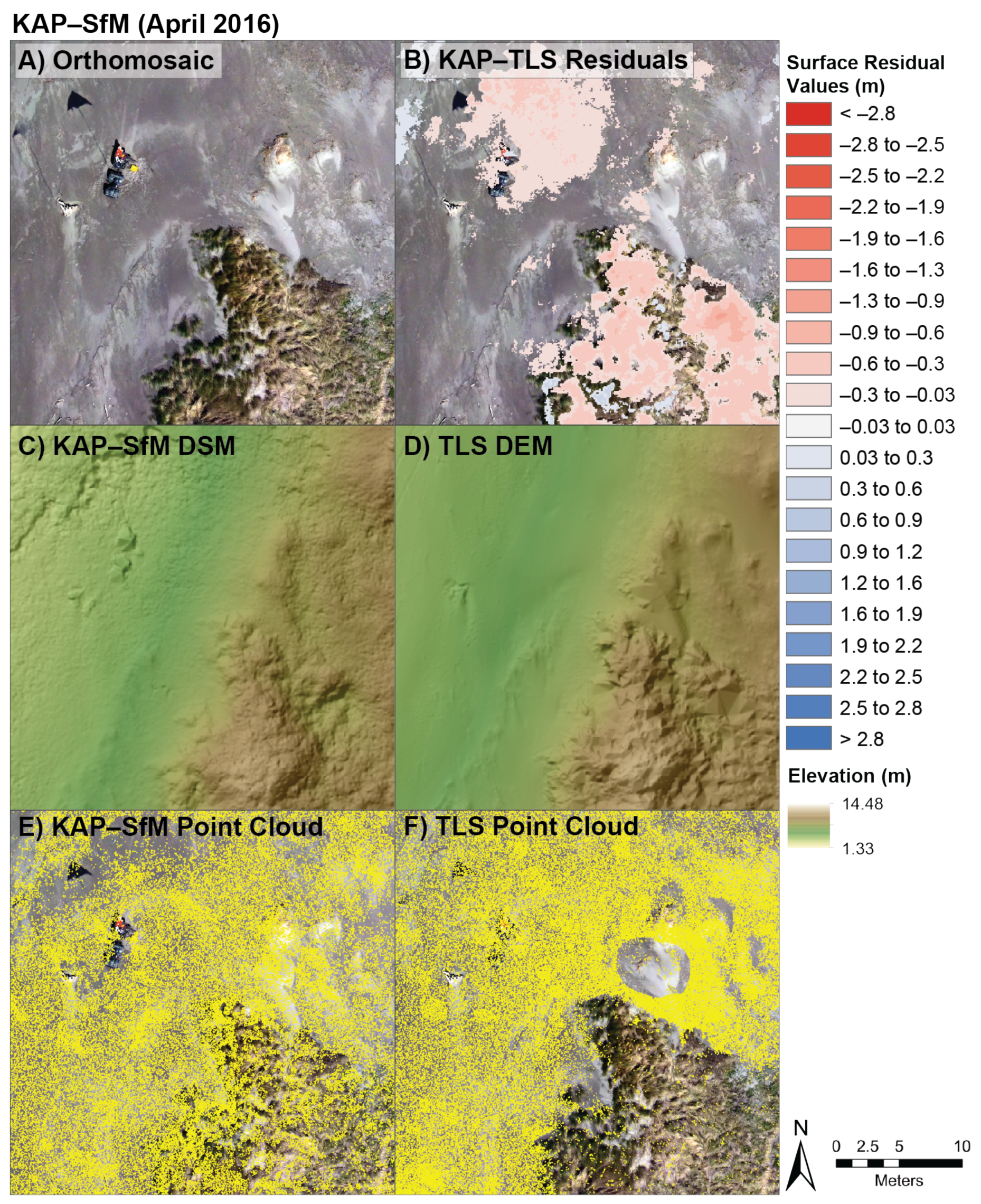
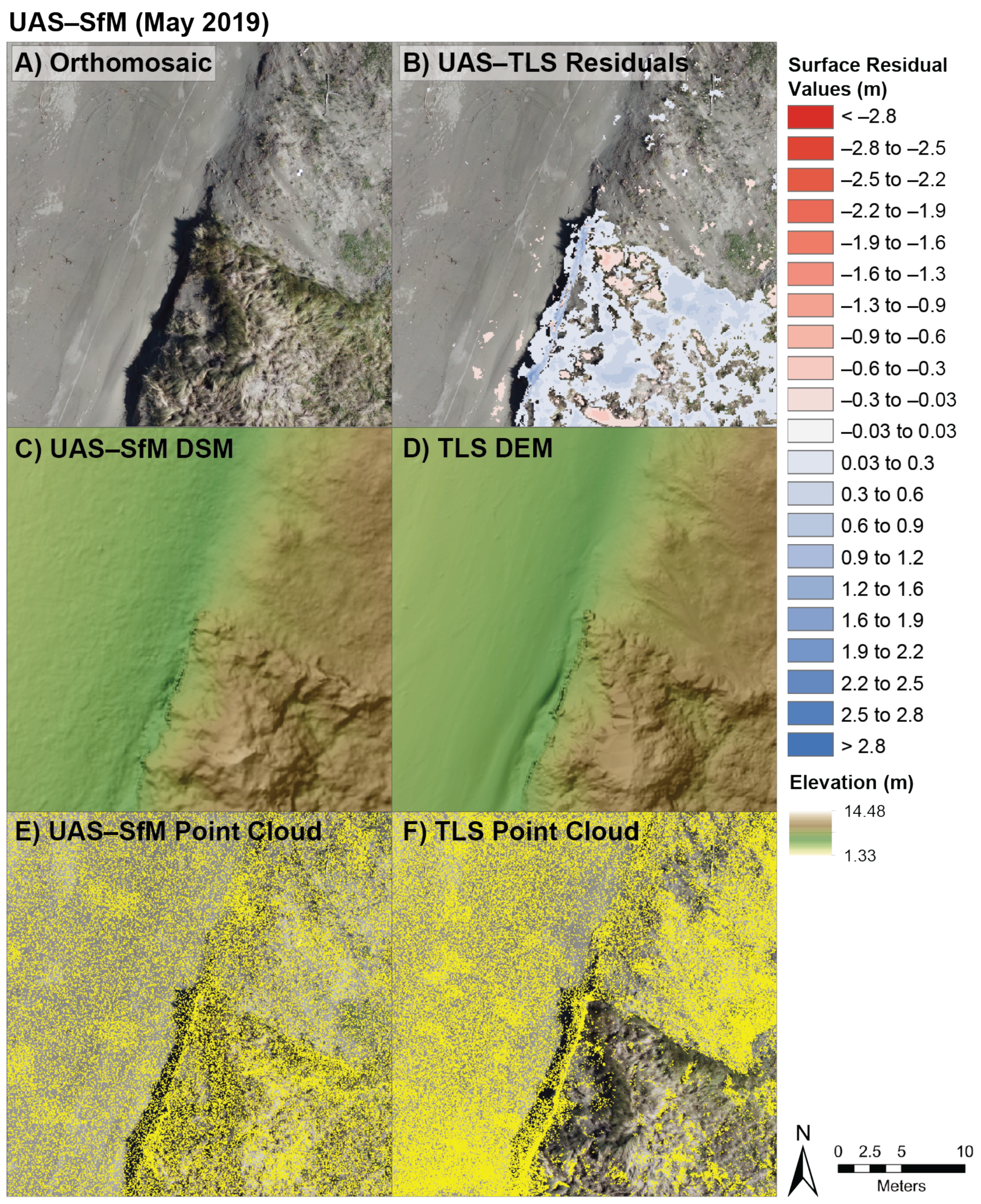
• Compare KAP- and UAS-SfM products against concurrently collected, higher resolution TLS reference surfaces to assess factors driving inter-platform differences.

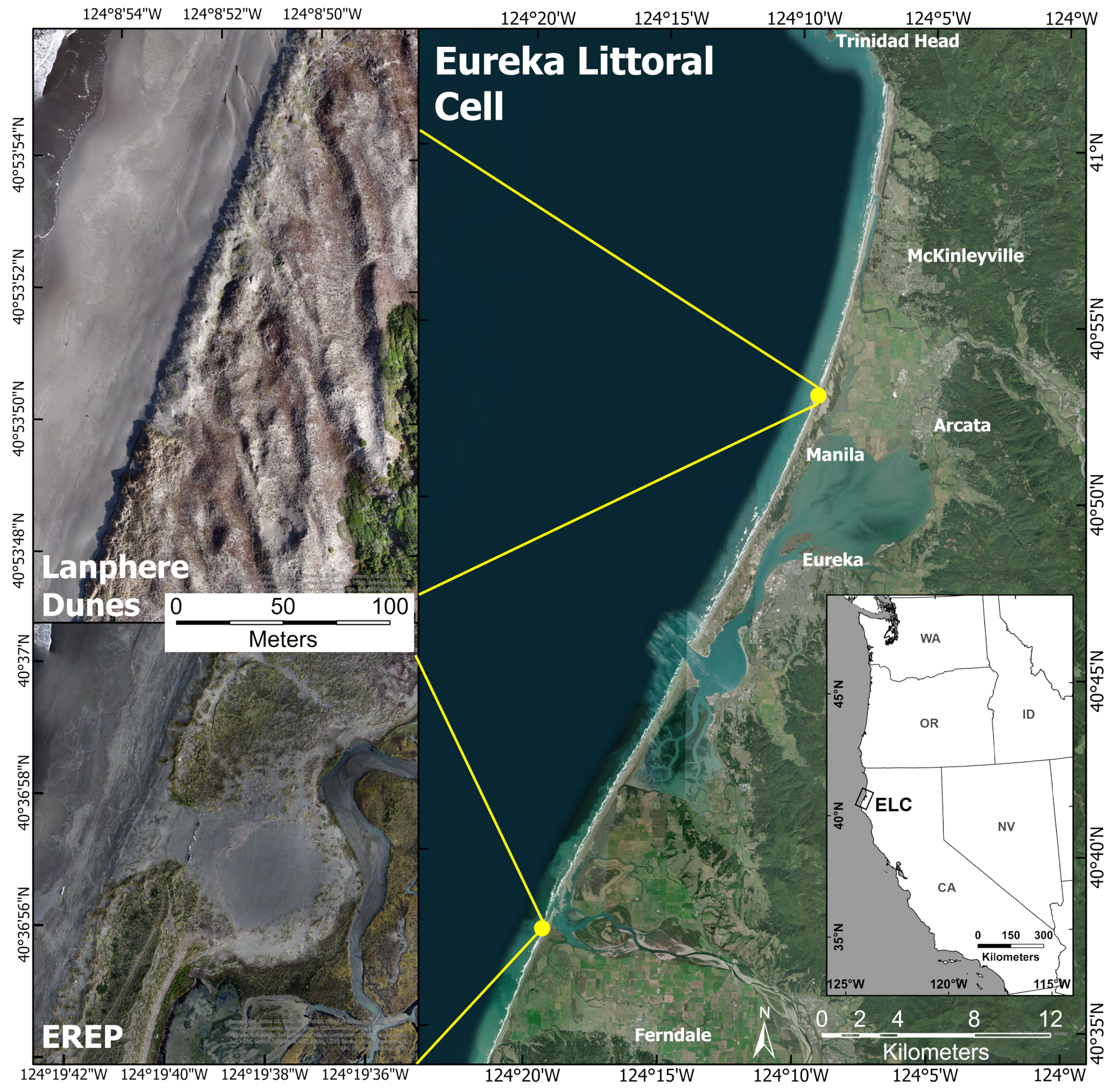
Our analyses utilize the GCD toolset [44,45,46] in ArcMap 10.7.1 to quantify volumetric change cumulatively, between surveys, and discretely, within each vegetation plot, as well as to quantify differences between concurrently collected datasets. We also provide discussion on the logistical considerations and concerns when utilizing multiple platforms and for using UAS for coastal geomorphic research. Our goal is to improve considerations for coastal geomorphic assessments with UAS, while furthering discussions focused on the impact of vegetation on foredune morphodynamics and the impact that different platforms can impart within such comparisons. Finally, we discuss the role of uncertainty in topographic differencing and how different forms of uncertainty should be considered to inform on realistic geomorphic change.

2. Study Area

2.1. Eureka Littoral Cell

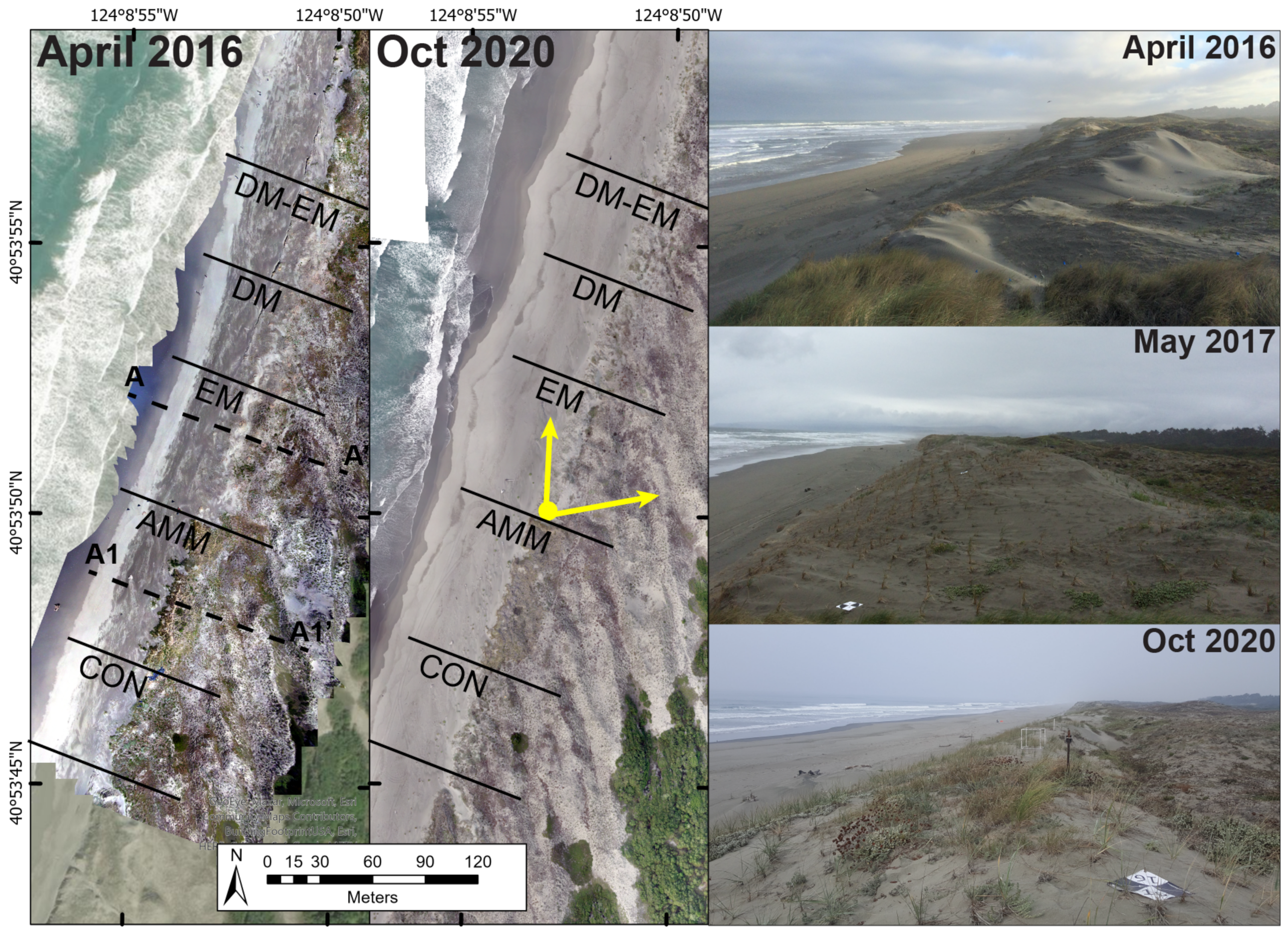
The Eureka Littoral Cell (ELC) is a 60-km stretch of coast in northern California that lies between Trinidad Head in the north and False Cape in the south, near Ferndale (Figure 1) [47]. The ELC is located to the north of the Mendocino Triple Junction where the Pacific, Gorda, and Juan de Fuca plates meet [48] and the Cascadia Subduction Zone converges with the San Andreas Fault (see Figure 1 in Patton et al. [48] for detailed tectonic map). This unique, complex geologic setting influences relative sea level trends in the region that, coupled with current rates of eustatic sea level rise, result in roughly 2.53–5.84 mm yr⁻¹ of relative sea-level rise [28,48,49]. The Eel and Mad Rivers are the dominant sources of sediment to the ELC, although sediment budgets and littoral drift dynamics are poorly understood within the study area [47,50]. Littoral drift is believed to be dominated by northerly driven storm waves and currents in the winter and southern wind wave-driven transport during the summer [28]. Wind and wave directions vary seasonally, with formative transport winds and dominant waves coming from the north-northwest between May–October and southeasterly winds with west-northwesterly waves between November–April [27,28] (Figure 2). The barrier and dune systems along the ELC also play an important ecological role, hosting a variety of migratory and native birds, mammals, and fish species including the endangered Western snowy plover, tundra swans, bald eagles, Aleutian geese, river otters, and steelhead trout [51,52]. Finally, the beaches and dunes of the ELC provide an array of ecosystem services that include erosion and flood control, habitat for endangered and endemic species, outdoor education and recreation, aquaculture, and sites of cultural importance.

2.2. Lanphere Dunes

The Lanphere Dunes are located within the Humboldt Bay National Wildlife Refuge and are managed by the United States Fish and Wildlife Service (Figure 3). The Lanphere Dunes feature a continuous, 7–10 m high foredune ridge and an extensive transgressive dune complex that extends up to ∼600 m inland. This site has been the focus of decades of ecosystem restoration work and efforts to remove Ammophila arenaria (European beach grass), an invasive plant species, which began in the 1980s [55]. Lanphere is also considered among the first documented efforts to prioritize ‘dynamic restoration’ practices, where invasive species are removed and natural vegetation is replanted on the foredune as a means of restoring natural biological and geomorphic (aeolian) processes [25]. A. arenaria was originally planted in 1901 to help stabilize the foredune and protect sites of local economic importance but rapidly spread along much of the ELC shoreline [56]. Removal of A. arenaria at the study site has involved manual pulling, drying, and burning of the biomass. Native species have been replanted across the site including Elymus mollis (dune grass or sea lyme grass) and the dune mat herbaceous alliance (including Abronia latifolia and Ambrosia chamissonis) (Figure 3). Replanting was completed between winter and spring of 2016-17 with three different revegetation strategies used: (1) mature E. mollis planted with 1 m spacing, (2) mature dune mat randomly distributed across the foredune, and (3) a mixed plot of E. mollis and dune mat. A plot of A. arenaria and a plot of naturally occurring native vegetation were maintained as control plots. E. mollis and dune mat were chosen as species that occupy different ecological niches during foredune evolution. E. mollis is a taller (<1 m) grass, considered to be a leading-edge dune builder that colonizes bare sand [57]. The dune mat species represent low-lying, prostrate herbs and subshrubs.

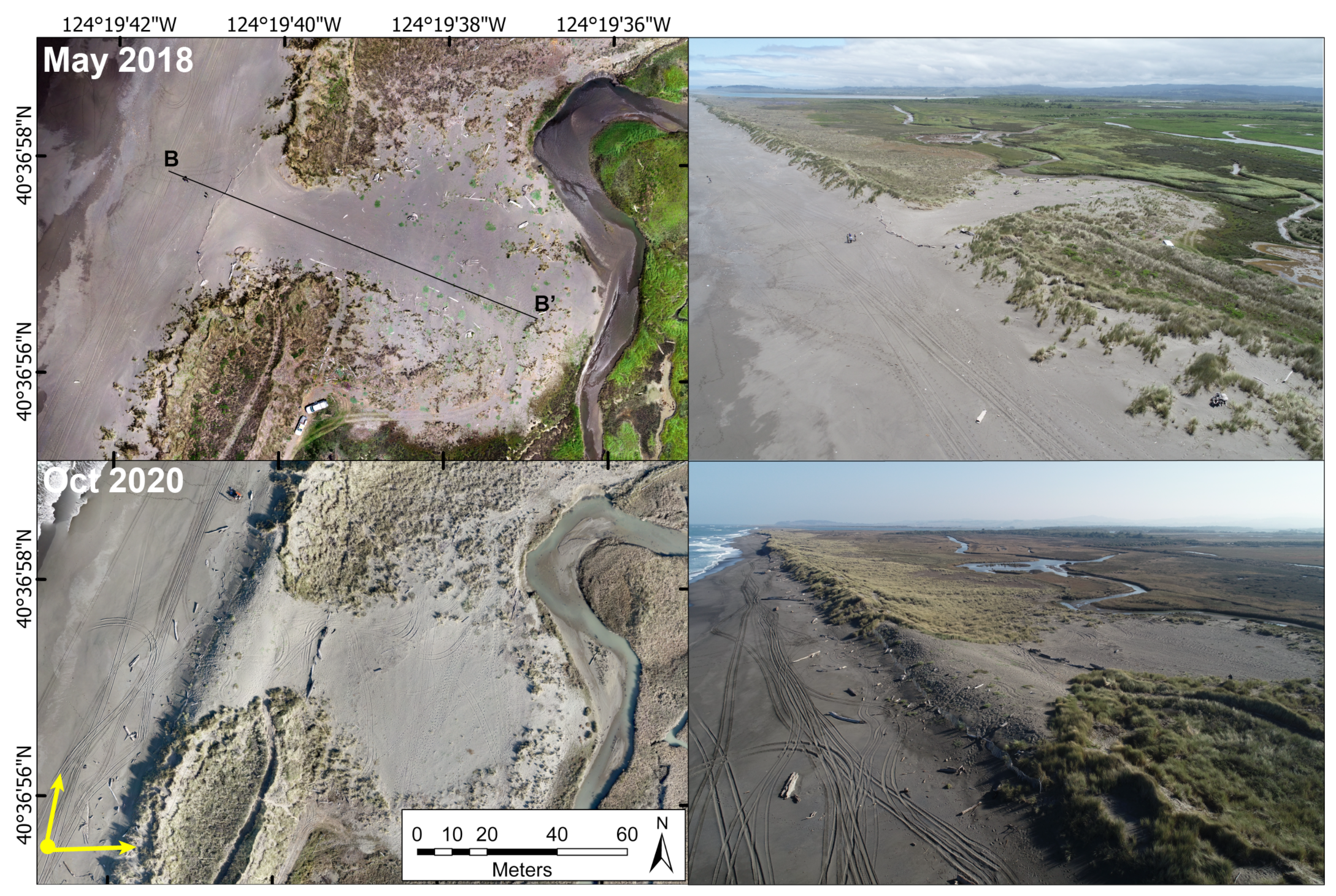
2.3. Eel River Estuarine Preserve Dunes

The Eel River Estuary Preserve (EREP) is a 5 km² nature preserve located west of Ferndale, CA. The preserve extends along 5.5 km of coastline, with 4.8 km of foredune, between the mouth of the Eel River to the north and Centerville Beach to the south. Tidal sloughs, wetlands, and agricultural fields represent the remaining preserve area. A. arenaria is prevalent on the EREP foredunes and has resulted in a taller, more peaked, and narrower dune form compared to natively vegetated dunes, leaving them susceptible to scarping during erosive events [20,27,28,58]. The beach is narrow (typically <50 m), steep, and experiences a high-energy wave regime with 20% of winter wave heights exceeding 4.0 m [59,60]. A major wave breaching event occurred during the summer of 2004 which resulted in landward deposition of sand into the backdune wetland forming an overwash fan [61,62,63] (Figure 4). The foredune was mechanically rebuilt with heavy machinery during the summer of 2018. Plans to replant the foredune with native vegetation have not been completed, however, some dune mat species were planted in the summer of 2019 [64]. As a result, much of the foredune remained unvegetated by October 2020. Restoration goals at the EREP site focused on the reconstruction of a foredune to reinstate a continuous foredune ridge and protect landward agricultural and ecosystem interests from flooding [64].

3. Materials and Methods

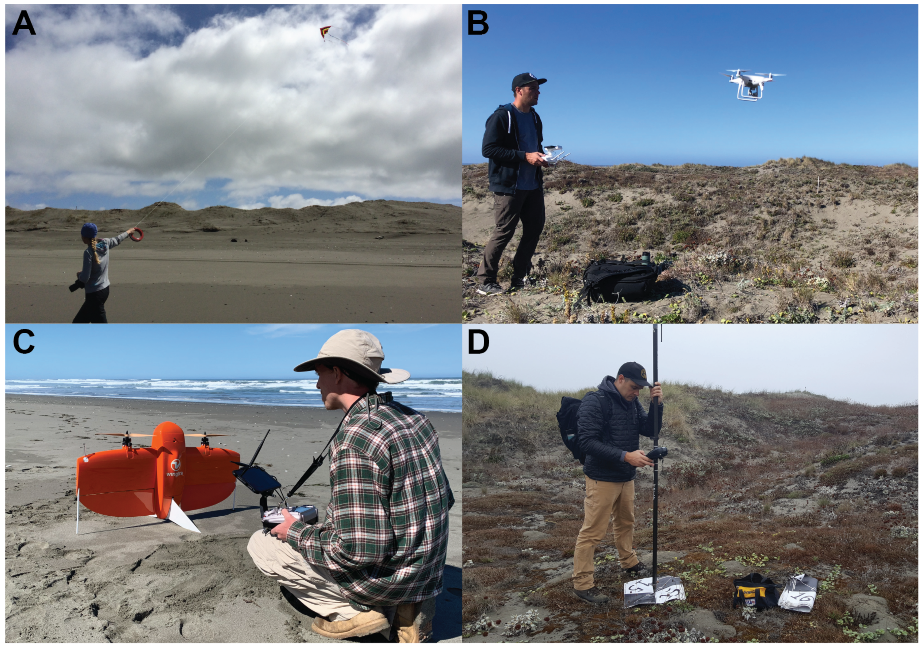
3.1. KAP and UAS Campaign Specifications

Three different uncrewed platforms were used to conduct aerial surveys (Figure 5). KAP data were only collected at the Lanphere study site, but were collected on six different occasions between 2016–17 (

Table 1. Collection specifications for all flights at the Lanphere and EREP study sites. DJI Phantom 4 Pro (DJI P4P) has been abbreviated. An asterisk (*) next to a date signifies a concurrently collected TLS campaign. GCPs were used for the 20 May 2019 EREP campaign because of an error with the onboard PPK system. September 2019 average wind speeds were informed by an anemometer at the time of collection, because the NBDC Station (46022) was not in operation for a six-month period in 2019.

	Collection Date (M/D/Y)	Platform	Model	Camera	Alt. (m)	GSD (cm/pix)	Images Used	Geocorrection Method	Avg. Wind (m/s)	Total Uncertainty (m)
Lanphere	4/30/2016 *	Kite	N/A	GoPro Hero4 12MP/4K)	32.1	1.79	1804	GCPs (n = 10)	3.8	0.072
	7/5/2016				76.9	8.06	926		5.8
	9/28/2016 *				44.1	2.59	3313		6.4
	1/6/2017				24.9	2.75	1028		5.6	0.021
	3/22/2017				43.9	4.3	1082		6.0	0.021
	10/3/2017 *				41.2	2.05	1215		9.3
	10/6/2018 *	Quadcopter	DJI P4P	20 MP	68.7	1.73	545	GCPs (n = 14)	3.2	0.029
	5/19/2019 *	Fixed-Wing	WingtraOne	Sony RX1RII (42 MP)	108	1.37	1010	PPK	5.6	0.027
	9/16/2019 *				101	1.28	1394		∼1.5	0.031
	10/8/2020 *				97.9	1.25	1387		3.1	0.020
EREP	5/23/2018	Quadcopter	DJI P4P	20MP	65.7	1.67	266	GCPs (n = 11)	2.1	0.032
	10/8/2018				52.5	1.37	418	GCPs (n = 11)	6.0	0.031
	5/20/2019	Fixed-Wing	WingtraOne	Sony RX1RII (42 MP)	104	1.32	526	GCPs (n = 12)	4.8	0.033
	9/17/2019				108	1.37	386	PPK	∼4.5	0.037
	10/9/2020				103	1.32	407		2.4	0.032

). Acquisition methods were consistent across all six collections. Ten ground control points (GCP) were placed throughout the site (five on the beach and five on the foredune) and their locations were recorded using a Trimble R10 RTK-GNSS to ensure accuracy. A 12MP/4k GoPro Hero 4 camera was attached to a Delta Kite (https://store.publiclab.org/) with a 3D-printed gimbal to try to maintain nadir viewing angles (Figure 5A). Kite campaigns were flown with the camera set to video mode to ensure sufficient coverage of the study area. The kite was walked in a U-shaped path, first north across the beach over the extent of the study site and then back across the seaward toe of the foredune. Still images were then extracted from the videos at 60-frame (1 s) steps in Agisoft Metashape.

Similar to the KAP methods, GCPs were deployed for the DJI Phantom 4 Pro quadcopter UAS surveys. GCPs were randomly distributed in high and low points across the study area to reduce the possibility of doming issues [65] and account for the complexity of the terrain [4]. The GCP locations were also recorded using a Trimble R10 RTK-GNSS. We used the Pix4Dcapture application to pre-program our acquisition campaign, which was a double-grid pattern at an altitude of 60 m, with 70% front and side camera overlap, following suggested standards [4]. GCP positions were corrected and refined using the National Oceanic and Atmospheric Administration’s (NOAA) online positioning user service (OPUS) solution (https://geodesy.noaa.gov/OPUS/).

The second UAS was a WingtraOne fixed-wing vertical take-off and landing platform. Compared to the Phantom 4 Pro, the WingtraOne can be flown at higher altitudes, achieve a finer ground sampling distance (GSD), has longer flight times (∼40 min), and is equipped with post-processing kinematic (PPK) correction capabilities. A Trimble R10 base station was run in static collection mode immediately prior to and until the end of each flight, fully encompassing the flight duration. At the start of processing, base station files were corrected with a NOAA-OPUS solution that is written to the image data for use in SfM reconstruction in Agisoft Metashape (V1.6.3.10732). Campaigns were flown at ∼100 m and achieved GSD values between 0.0127–0.0135 m. The WingtraOne collected photos in a nadir camera angle with a Sony RX1RII 42 MP full-frame camera. A major advantage of utilizing a full-frame camera is a reduction in radial pixel distortion that is often typical with conventional domed (or fish-eye) camera lenses [66].

3.2. Post-Processing and Intercampaign Alignment

Post-processing protocol remained consistent across each campaign, with the only deviation being the still image extraction from the 4k video footage required for the KAP datasets. Projects were processed in Agisoft Metashape and aligned using high parameters with a key point limit of 40,000 and a tie point limit of 4000. Once aligned, the point cloud was filtered using the Gradual Selection tool, taking 10–15% of the total points from reprojection error, reconstruction uncertainty and projection accuracy during each iteration of the tool, until there is less than a 10% change in marker accuracy values after point removal. A dense cloud was generated using the high setting and mild depth filtering, and with a calculation of point confidence. Point confidence is a metric of how many depth maps were used to generate a given point in the dense cloud [67]. After the dense cloud was processed, all points below a confidence threshold of 10 were removed from the point cloud. Confidence filtering followed suggested methods in Agisoft Support forums for improving dense cloud products and methods by Bayley and Mogg [68].

Most of the UAS and KAP datasets at the Lanphere study site were aligned to TLS bare earth point clouds to ensure the datasets were accurately positioned in space (Table 1). TLS data were collected using Riegl VZ-1000 (April 2016–September 2016) and VZ-400i (October 2017–October 2020) scanners and integrated with a Trimble R10 RTK-GNSS for precision alignment. Campaigns were processed in Riegl RiSCAN Pro to align scans, filter excess points, remove vegetation, and align campaigns to each other. KAP- and UAS-SfM point clouds were then imported into RiSCAN Pro, manually cleaned and filtered to remove spurious points and vegetation, and aligned using the multi-station adjustment tool, which searches for similarity between extracted planes in the point clouds. Point clouds for TLS, UAS, and KAP data were then exported for further processing in ESRI ArcMap 10.7.1. Point clouds were converted to rasters with 0.1 m cells using inverse distance weighted interpolation (to assign cell values) and linear interpolation (to fill data voids). Rasters were processed using a consistent, rounded (whole number) extent to ensure concurrency during change detection processing. Ensuring concurrency during this step avoids cell offsets that would result in systematic volumetric errors (e.g., “slivers” between non-aligned cells).

3.3. Budgeting for Uncertainty

Uncertainty is important to consider when utilizing close range-remote sensing data for geomorphic assessments. Here, we use the term “uncertainty” to refer to an undefinable level of possibly undetectable change, whereas “error” would refer to the difference between a dataset and a higher accuracy reference dataset [69]. Calculating uncertainty can be a subjective task with little in the way of “standard operating procedures,” making the development of an error budget an ambiguous task. We took precautions to include multiple sources of uncertainty to identify possibly insignificant volumetric change (Table 1). We also performed a comparison between our KAP- and UAS-SfM-derived surfaces and TLS DEMs that were concurrently collected, similar to the approach of Guisado-Pintado et al. [32]. This comparison helps to highlight areas of concern or higher uncertainty against an arguably more accurate dataset.

Uncertainty can arise from multiple contributing factors or sources. For example, Hon [70] and Sherman [71] discuss four types of error that complicate accurate results and inflate uncertainty. These include Type 1 (background theory), Type 2 (equipment), Type 3 (observational reports) and Type 4 (theoretical conclusions) errors. The driving uncertainty for using UAS platforms to detect and quantify geomorphic change would typically be Type 2 error, related to assumptions regarding equipment precision, and Type 3 error, related to the differences between a measured and true values. For instance, uncertainty budgets could include error resulting from the accuracy of the equipment, the root mean square errors (RMSE) generated by the alignment of SfM point clouds to reference point clouds, and the positional and vertical accuracy of GCPs. In this way, uncertainty budgets distill down into two primary forms of uncertainty that influence the accuracy of geomorphic change detection: (1) ”Collection uncertainty” that results from the acquisition of data and from equipment in the field, and (2) ”Processing uncertainty” that results from processing, alignment, and refinement of datasets following collection. Combined, these forms of uncertainty result in positional and vertical deviations within point cloud datasets that inflate the minimum level of detection for topographic differencing and decrease realistically measurable geomorphic change.

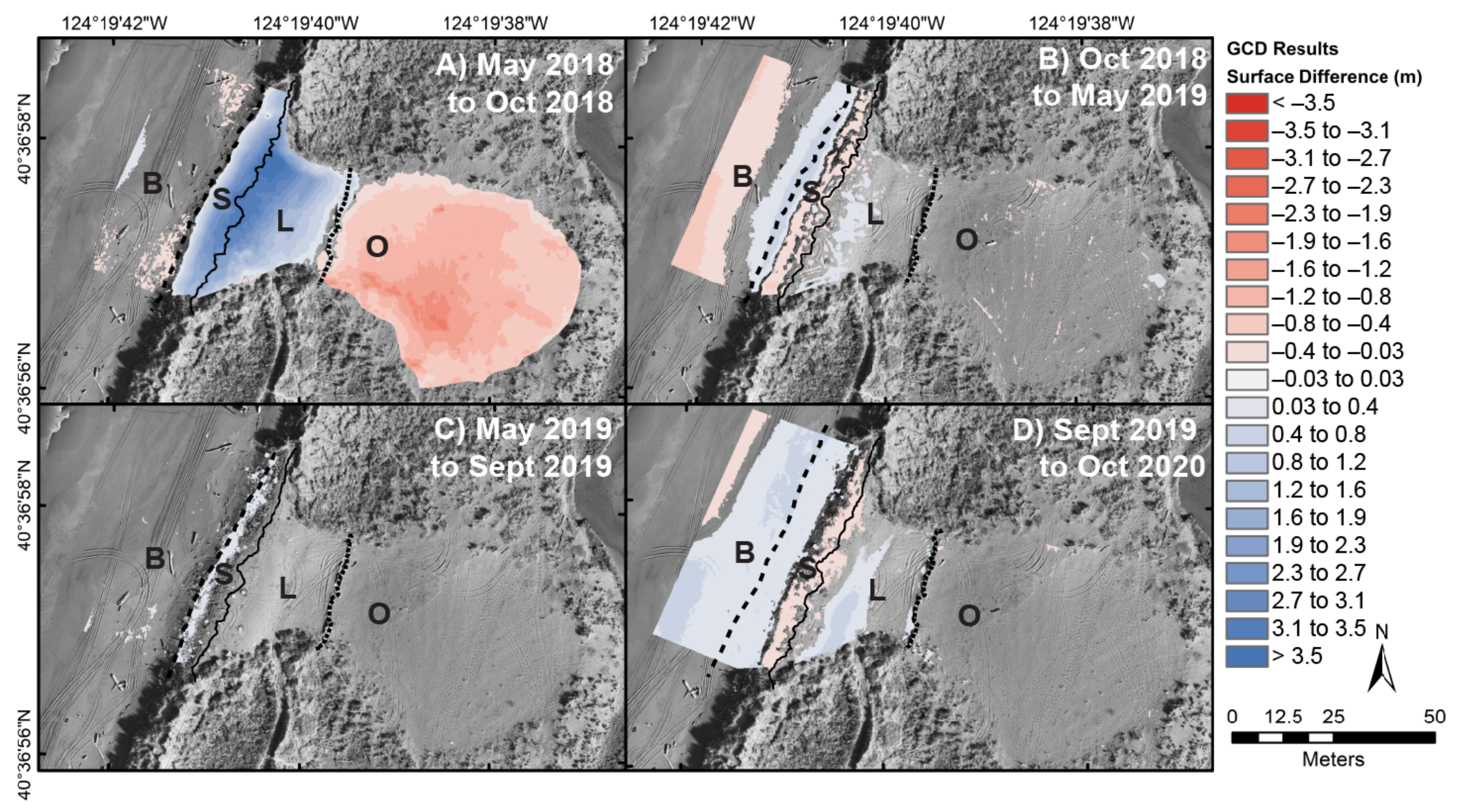
3.4. Geomorphic Change Detection

Repeat high-resolution UAS-SfM datasets can be compared to create DEMs or DSMs of difference that provide insight into spatial-temporal volumetric changes and landform morphodynamics. Simply, this style of change analysis subtracts a co-located older surface (t₁) from a newer surface (t₂) [72,73]. Positive values indicate an increase in surface elevation from the older time to the newer time, and vice versa. However, discerning what is “real” change can sometimes be difficult, as DEM or DSM outputs are subject to varying types and degrees of uncertainty [5,45,69,72,73]. We utilized the GCD toolset developed by Riverscapes Consortium ([44,45,46], http://gcd.riverscapes.xyz/) to conduct our change analysis. The GCD toolset imports surface rasters and allows users to generate hillshade, slope, and error rasters to improve analyses. The “error” raster is informed by user input and typically functions as a cumulative error estimate that is based on survey instrumentation constraints. An error layer is generated for each raster and the propagated error is applied to each cell using Equations (7) and (12) from Lane et al. [73]:

$${\sigma }_c=\sqrt{{\sigma }_1^2+{\sigma }_2^2}$$

(1)

$$t=\frac{z_{t2}-z_{t1}}{{\sigma }_c}$$

(2)

where $\sigma$${}_c$ is equal to the root sum of squares of uncertainty for each change interval and z is the elevation of the raster cell for the newer ($t_2$) and older ($t_1$) time steps. The output is a t−statistic that, assuming normal distribution, can be used as a thresholding level where values of t > 1.96 (confidence interval of 95% for a two-tailed t-test) are kept as change that is significant. Values that fall below the confidence threshold are removed from the output change raster, providing a minimum level of detection to improve the likelihood that significant change was captured. Primary outputs include raw and thresholded depth of change, area of change, and volume of change.

The GCD toolset also allows users to input masks to subsample areas of interest. For this study, three geomorphic units (beach, seaward slope of the foredune, landward slope of the foredune) and five vegetation units (native control—CON, A. arenaria—AMM, E. mollis—EM, dune mat—DM, and a mix of dune mat-E. mollis—DM-EM) were delineated by building upon methods previously used at the site by Rader [74]. Boundaries between the geomorphic units were defined using landscape metrics, such as slope breaks, slope aspect, and vegetation [74]. The crest of the foredune represented the boundary between the seaward and landward slopes, and was automatically delineated for each survey using the Basin tool in the ArcToolbox Spatial Analyst package. Our approach also used a red-relief image map [75] that combines slope with positive (surface convexity) and negative (surface concavity) topographic openness. Visualization of DEMs typically uses colored, semi-transparent elevation data over a shaded relief map. An advantage to delineating geomorphic boundaries using the red-relief method over a shaded relief layer is that it reduces potential bias from shadows cast in complex terrain, such as in a coastal dune complex. We utilize this method to better visualize the seaward and landward toes of the foredune. We acknowledge that the position of the seaward and landward toes can be considered subjective [76], but took precautions to reduce potential bias by requiring a single analyst to digitize these features to determine a best representative boundary for each. In some cases, when the seaward toe was eroded and an erosional scarp was present, the base of the scarp was used as the seaward extent of the foredune. The subset areas applied to each GCD output reference the earlier collection in the timestep and quantify change from the initial state of each comparison.

The two study sites provide a unique opportunity to compare GCD outputs in similar geomorphic systems, with a variety of different, site-dependent factors impacting uncertainty and the accuracy of results. The two primary differences between the Lanphere and EREP sites are the possible impact of vegetation on the surface models and the potential for quantifying variance from higher accuracy reference datasets. The EREP foredune was not vegetated after reconstruction of the dune, whereas the Lanphere foredune was stripped of its vegetation and replanted with native species that vary in shape, height, and coverage. The Lanphere site compared concurrently collected aerial (KAP- and UAS-SfM) surfaces to TLS bare earth surfaces. We consider the TLS data to be of higher accuracy and with more consistent geocorrectional constraints, providing a reference surface to quality check the aerial data. While we did not have the ability to directly compare a KAP-SfM surface to a concurrently collected UAS-SfM surface, the ability to compare to a TLS reference surface allows us to make inferences regarding the accuracy of SfM reconstruction between aerial platforms. The EREP site does not have a similar reference dataset to compare against, but the platforms used (quadcopter and fixed-wing) employed more rigorous collection strategies, like those at Lanphere.

3.5. Quantifying Vegetation

Quantifying vegetation was not necessary at the EREP site, as vegetation was not present on the dune until the summer of 2019. However, assessing vegetation at Lanphere was crucial for comparing sediment erosion and deposition patterns in the treatment plots to growth and propagation of plant cover. Automated and semi-automated classification methods were explored, however, due to similarities in color between the sand and vegetation during some collection intervals, a manual approach was chosen. This manual approach allowed the two main treatment methods of interest (E. mollis and the dune mat herbaceous alliance) to be distinguished. Analysts digitized vegetation across the treatment plots in two ways: (1) E. mollis plants were digitized with a point feature class to develop a count using each orthomosaic image, and (2) dune mat plants were digitized as polygons to calculate an area of coverage and then split using the Intersect tool in the Analysis Toolbox of ArcMap 10.7.1 and the appropriate geomorphic unit and treatment plot boundaries. We did not try to distinguish between dune mat herbaceous alliance species, because the assemblage is made of over 50 different species and many take on similar low-lying forms. Intersecting the dune mat feature class allowed area per plot and geomorphic unit to be accurately subdivided, even if the plant extended across boundaries.

After vegetation was digitized, we compared the average state of vegetation (% cover), relative to the maximum recorded vegetation cover by plot. For example, if the seaward slope of the DM-EM plot recorded 100 E. mollis plants and the maximum observed across all time steps for that plot was 500 plants, that observation would be assigned a value of 20%. Similarly, if the dune mat area occupied 200 m² and the maximum observed area was 250 m², the observation would be assigned a value of 80%. These values were averaged for each plot observation interval to provide a proxy for the state of vegetation propagation. In the example provided, the vegetation state would equal 50%. In this way, values were normalized to provide plot- and vegetation type-specific context for interpretation of patterns between vegetation development and sediment erosion and deposition. These values were then compared to area-normalized volumetric change by matching the vegetation value with the later date in each GCD interval. A simple linear regression model of the area-normalized volumetric change (m³ m⁻²) (dependent) against the state of vegetation (%) (independent) was calculated using the R package ‘ggplot2’ [77].

4. Results

4.1. Uncertainty Assessments for KAP and UAS Datasets

Uncertainty budgets were compiled for each survey to inform on the possible impact of uncertainty on geomorphic change calculations. Budgets were generated using reported GCP or total XYZ error, reported RTK accuracy, and RMSE from point cloud alignment. GCP error, total XYZ error, and RMSE from point cloud alignment were variable numbers that were based on each survey. RTK accuracy was assumed a constant that was informed by industry reported values and the Trimble R10 datasheet. The final cumulative value was then input into the GCD tool as a uniform error value applied to each pixel of the raster surface (Table 1). Uncertainty values ranged between ±0.02–0.04 m for all intervals except the April 2016 KAP dataset (±0.072 m). Uncertainty budgets for surveys compared in the GCD tool were then propagated to calculate a minimum level of detection, which acted as a threshold value to remove points that fell outside of a confidence interval of 95%.

Half of the KAP-SfM datasets at the Lanphere site were successfully processed, aligned, and included as GCD intervals. The July and September 2016 and October 2017 campaigns were not used in the final datasets, as systematic collection errors led to poor surface reconstruction during SfM processing. Poor reconstruction of the beach, impacted by surface homogeneity, waves, and increased moisture, led to higher surface variability and greater point cloud diffusion, compared to TLS reference surfaces (Section 4.2). There were also tidally-driven collection constraints that limited the seaward extent that the pilot could walk the kite and led to fewer images for pattern matching towards the seaward edges of the area of interest. The September 2016 KAP-SfM point cloud was domed and attempts to reconcile the dataset were unsuccessful. Doming refers to the deformation of an SfM point cloud in a radially-distorted manner [78]. The July 2016 and October 2017 KAP-SfM point clouds exhibited low point confidence, with large portions of the beach and foredune removed during the dense cloud filtering stage. All three of these KAP datasets were collected during high wind conditions (Table 1), which might have contributed to their respective shortcomings due to variable overlap, focus, or the number of images removed. Uncertainty for the KAP-SfM datasets included the highest calculated budget (±0.072 m) in April 2016. Uncertainty budgets for the January and March 2017 campaigns were lower than the other KAP datasets (±0.021 m). However, TLS campaigns were not concurrently collected with these two datasets and September 2016 and May 2017 TLS campaigns were simultaneously used to align the point clouds, representing a deviation in alignment methods.

All of the UAS-SfM datasets for the Lanphere and EREP sites were successfully processed and used to derive GCD outputs. Unlike the KAP-SfM datasets, the UAS-SfM datasets recreated the beach with higher point confidence, doming was not apparent, and the surveys benefited from pre-programmed flight planning and onboard GPS systems to ensure effective and consistent image acquisition. Wind speeds did not appear to impact the UAS surveys in the same manner as the KAP surveys, despite moderate wind speeds for many of the fixed-wing collections (Table 1). Better flight stability control and onboard sensors regulated the fixed-wing flights and reduced overall pitch-yaw-roll variability. The fixed-wing UAS would automatically terminate acquisition if winds were too high to ensure safe, reliable flight control and data acquisition. Uncertainty for the UAS-SfM datasets ranged from ±0.020–0.031 m at the Lanphere site and ±0.031–0.037 m at the EREP site.

4.2. Differences between Platforms

Most (7 of 10) of the KAP and UAS surveys at the Lanphere site had concurrent TLS surveys, which allowed us to characterize differences between surfaces constructed with aerial datasets and the TLS surfaces. We consider the TLS surfaces to provide a higher accuracy baseline reference for estimating uncertainty residuals in the KAP- and UAS-SfM products. After removal of the September 2016 and October 2017 KAP-SfM datasets, the five remaining datasets (one KAP, one quadcopter UAS, and three fixed-wing UAS) were compared against the TLS surfaces. The GCD tool was used to compare these surfaces, with methods similar to those used by Guisado-Pintado et al. [32]. Positive or negative values represented residuals between the aerial platform data and the TLS-derived surface that characterized areas of deviation or greater uncertainty in the KAP- or UAS-SfM surfaces. Output residual values were summed by (1) vegetation treatment plot (as a combination of seaward and landward slope units) and (2) geomorphic unit (without vegetation delineation) (

Table 2. Comparison between concurrent aerial and TLS datasets, subset by geomorphic unit and vegetation type. An additional subset for the seaward and landward units is provided for only the EM, DM, and DM-EM (restored) plots.

	April 2016 (KAP)		October 2018 (UAS)		May 2019 (UAS)		September 2019 (UAS)		October 2020 (UAS)
Vegetation/ Geomorphic Unit	$\Delta$ Area (%)	Residual Difference (m3m−2)	$\Delta$ Area (%)	Residual Difference (m3m−2)	$\Delta$ Area (%)	Residual Difference (m3m−2)	$\Delta$ Area (%)	Residual Difference (m3m−2)	$\Delta$ Area (%)	Residual Difference (m3m−2)
CON			9.7	0.004 ± 0.03	14.2	0.011 ± 0.03	11.6	0.009 ± 0.03	14.0	0.009 ± 0.03
AMM	61.7	−0.149 ± 0.07	57.7	0.103 ± 0.03	51.3	0.065 ± 0.03	52.5	0.064 ± 0.03	43.8	0.084 ± 0.03
EM	27.6	0.058 ± 0.07	8.0	0.009 ± 0.04	4.9	0.002 ± 0.03	12.2	0.014 ± 0.04	5.9	0.006 ± 0.03
DM	23.6	0.023 ± 0.07	2.1	0.001 ± 0.04	4.0	0.001 ± 0.03	3.3	0.003 ± 0.04	3.5	0.000 ± 0.03
DM-EM	24.8	0.026 ± 0.06	3.5	0.004 ± 0.04	9.7	0.009 ± 0.03	10.9	0.016 ± 0.04	8.9	0.000 ± 0.03
Beach	35.2	−0.054 ± 0.06	18.9	0.017 ± 0.04	23.4	−0.017 ± 0.03	8.2	−0.007 ± 0.04	0.3	0.000 ± 0.03
Seaward	31.6	−0.063 ± 0.06	18.4	0.031 ± 0.04	18.7	0.019 ± 0.03	21.1	0.026 ± 0.04	12.9	0.016 ± 0.03
Landward	52.6	0.064 ± 0.07	18.1	0.023 ± 0.03	18.4	0.022 ± 0.03	15.8	0.015 ± 0.03	26.9	0.043 ± 0.03
Seaward (Restored)	14.6	0.001 ± 0.06	5.2	0.006 ± 0.04	5.3	0.003 ± 0.03	11.3	0.014 ± 0.04	4.4	0.000 ± 0.03
Landward (Restored)	48.4	0.119 ± 0.07	4.6	0.004 ± 0.03	7.2	0.005 ± 0.03	4.1	0.004 ± 0.03	11.6	0.010 ± 0.03

). An additional subset was included to isolate the EM, DM, and DM-EM plots and distinguish the potential impact the denser vegetation of the AMM and CON plots may have had on reconstructed surfaces.

The AMM plot consistently featured the highest residual difference from the TLS surface and greatest area of difference (m²) between all compared surfaces. This plot was the most densely vegetated and the surface was not sufficiently visible, even after TLS post-processing, to allow for accurate and consistent reconstruction of the bare earth surface. Area of difference values, averaged across all concurrently collected comparisons, were lower for the CON, EM, and DM-EM plots, exhibiting differences of 12.4%, 11.7%, and 11.5%, respectively (Table 2). The DM plot featured the lowest variability from the TLS surface, with an average area of difference of 7.3%. The beach exhibited the highest difference from the TLS surface for the KAP dataset (17.2%) but the lowest of all geomorphic units for the Oct 2020 WingtraOne UAS dataset (0.3%). The seaward (20.6%) and landward (26.3%) slopes averaged similar variability (Figure 6). The KAP dataset had the lowest vegetation density for compared datasets but the highest variability amongst all platforms. All other UAS surveys had less than half the variability across restored plots with more than twice the vegetation density as the KAP dataset.

Positive residuals from the TLS surface signified a KAP- or UAS-derived surface that was higher than the TLS reference surface, and vice versa (Figure 6; Table 2). Residuals for the KAP-TLS comparison were the highest of all observed values for each vegetation type. Variance in the AMM plot was hindered by higher point variability and high vegetation density, resulting in the largest residuals of all plots and comparisons. Residuals for the UAS datasets were consistently positive for seaward and landward slope surfaces, with the greatest deviation in the AMM plot. Negative residuals for the beach unit in the May and September 2019 comparisons were driven by two different factors. A low (0.25 m) scarp, resulting from a previous high water event, was present along the beach during the May 2019 collection campaign. The TLS surface reconstructed this more accurately than the UAS surface because scan positions were strategically located to include the steep slope of the scarp, whereas the UAS-SfM process can struggle to recreate steep scarps, smoothing them out during processing [79]. The September 2019 beach featured more large woody debris than had been present in previous collections. The wood was removed more effectively through automated filtering in the TLS surface because of more low-angle points near the wood-ground contact, which was not reconstructed with as much detail in the UAS point cloud. However, nearly all UAS-TLS comparisons featured similar, low (<0.01 m³ m⁻²) positive residuals in the plots vegetated with all types of native species that were directly related to the presence of vegetation or the presence of an erosional scarp.

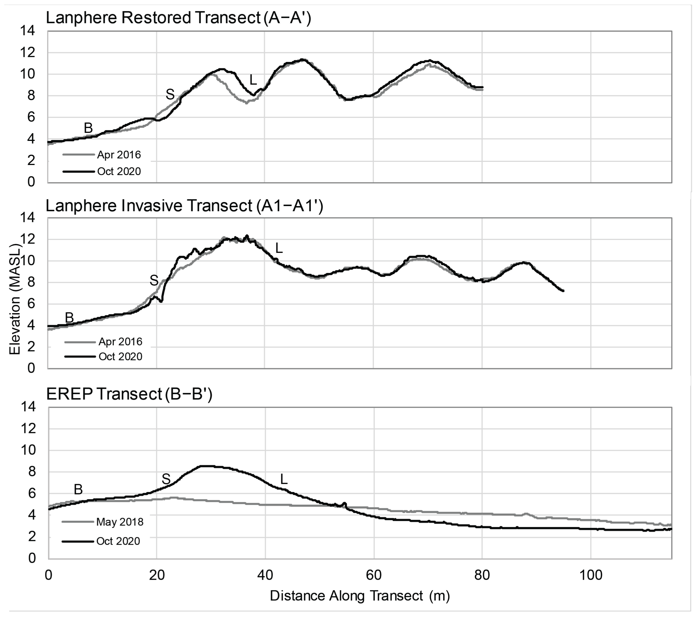
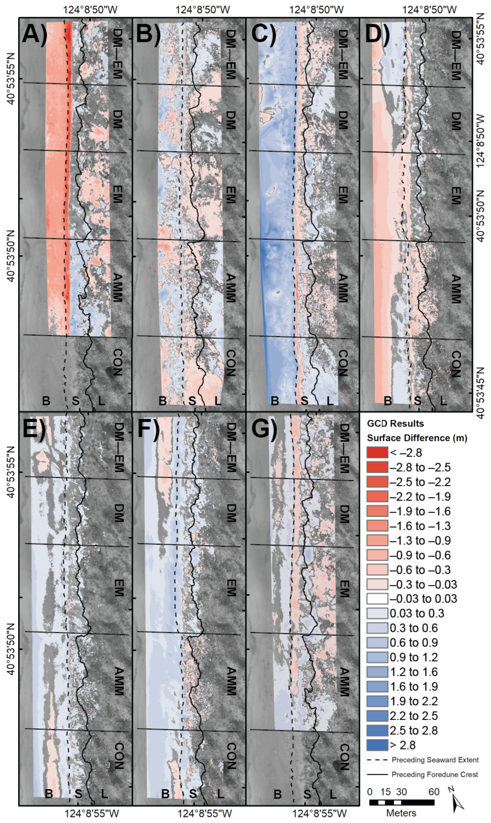
4.3. Geomorphic Change Detection

Spatial-temporal change detection results at the Lanphere and EREP sites were calculated using the GCD plugin [45] in ArcMap 10.7.1. The primary output from each interval was a raster surface of positive and negative surface elevation change values. This surface only included cells that were deemed significant at the 95% confidence limit, as informed by a t-test, and thresholded using the previously described uncertainty budgets (Section 4.1). Insignificant values were not removed from consideration and were included as potential change (±values), signifying results below the minimum level of detection. In this way, all calculated change for each interval is considered, but primary emphasis is placed on the values that were “significant”.

The Lanphere GCD intervals spanned from April 2016–October 2020 and included six collection intervals (Figure 7 and Figure 8;

Table 3. GCD outputs for all Lanphere intervals. This table is a complement to the visual depiction of GCD outputs in Figure 8.

Volumetric Change Normalized by Total Area (m3m−2)
Vegetation/ Geomorphic Unit	Apr 2016–Jan 2017	Jan 2017–Mar 2017	Mar 2017–Oct 2018	Oct 2018–May 2019	May 2019–Sept 2019	Sept 2019–Oct 2020	Apr 2016–Oct 2020
CON Beach		−0.02 ± 0.02	1.14 ± 0.04	−0.22 ± 0.03	0.12 ± 0.03	0.27 ± 0.03
CON Seaward		−0.15 ± 0.03	0.09 ± 0.03	−0.03 ± 0.03	0.07 ± 0.04	0.14 ± 0.03
CON Landward		−0.21 ± 0.03	0.22 ± 0.04	−0.01 ± 0.04	0.01 ± 0.04	0.01 ± 0.03
AMM Beach	−0.79 ± 0.07	0.04 ± 0.02	1.17 ± 0.04	−0.3 ± 0.03	0.16 ± 0.04	0.34 ± 0.04	0.39 ± 0.07
AMM Seaward	−0.09 ± 0.06	−0.02 ± 0.02	0.03 ± 0.03	−0.16 ± 0.04	0.09 ± 0.04	0.04 ± 0.03	0.18 ± 0.06
AMM Landward	0.17 ± 0.06	−0.01 ± 0.02	0.03 ± 0.03	−0.07 ± 0.04	0.03 ± 0.04	0.00 ± 0.03	0.11 ± 0.05
EM Beach	−1.12 ± 0.07	0.10 ± 0.02	1.06 ± 0.04	−0.35 ± 0.04	0.14 ± 0.04	0.36 ± 0.04	0.20 ± 0.07
EM Seaward	−0.44 ± 0.06	−0.03 ± 0.02	0.51 ± 0.03	−0.06 ± 0.03	0.07 ± 0.04	0.16 ± 0.03	−0.11 ± 0.06
EM Landward	−0.04 ± 0.05	−0.06 ± 0.03	0.23 ± 0.04	0.02 ± 0.03	0.05 ± 0.04	0.12 ± 0.04	0.32 ± 0.07
DM Beach	−0.94 ± 0.07	0.13 ± 0.02	0.71 ± 0.03	−0.14 ± 0.03	0.12 ± 0.04	0.15 ± 0.03	0.23 ± 0.07
DM Seaward	−0.52 ± 0.06	0.06 ± 0.02	0.06 ± 0.03	−0.01 ± 0.03	0.04 ± 0.04	0.17 ± 0.04	−0.12 ± 0.06
DM Landward	0.00 ± 0.05	−0.04 ± 0.03	0.04 ± 0.03	0.06 ± 0.04	0.06 ± 0.04	0.14 ± 0.03	0.28 ± 0.07
DM-EM Beach	−0.90 ± 0.07	0.08 ± 0.02	0.66 ± 0.04	0.08 ± 0.03	0.03 ± 0.03	0.10 ± 0.03	0.15 ± 0.06
DM-EM Seaward	−0.78 ± 0.06	0.05 ± 0.02	0.01 ± 0.03	0.01 ± 0.03	0.06 ± 0.04	0.18 ± 0.03	−0.21 ± 0.05
DM-EM Landward	−0.07 ± 0.06	0.05 ± 0.03	−0.01 ± 0.03	0.04 ± 0.04	0.02 ± 0.04	0.12 ± 0.04	0.15 ± 0.06

). No campaigns were conducted in spring 2020 due to travel restrictions during the COVID-19 pandemic. Strong winter storms between April 2016–January 2017 resulted in 0.9 ± 0.02 m of erosion of the beach. However, net deposition was recorded in almost all future timesteps, except October 2018–May 2019. A comparison between the April 2016–October 2020 surfaces showed that the beach accreted above April 2016 levels by 0.25 ± 0.068 m, while surface change on the seaward slope was negligible (0.025 ± 0.058 m). The winter of 2016–17 resulted in substantial erosion of the seaward toe of the foredune and, in some places, the development of an erosive scarp up to 3 m tall. Accretion on the upper beach between March 2017–October 2018 repaired most of the erosive scarp and minor accretion (0.06 ± 0.03 m) of the seaward slope was observed. October 2018–September 2019 recorded minimal net accretion, but the final timestep of September 2019–October 2020 recorded the highest accretion across all timesteps.

Next to the beach, the landward slope of the foredune recorded the most overall accretion resulting from sand ramp rebuilding and delivery up the seaward slope and over the crest. Erosion in the landward slope occurred between January–March 2017 (0.055 ± 0.028 m). The greatest accretion occurred in the March 2017–October 2018 (0.105 ± 0.034 m) interval, with minor accretion recorded from September 2019–October 2020 (0.071 ± 0.034 m) (Figure 8).

The EREP GCD results spanned from May 2018–October 2020 and the landscape was partitioned to include a fourth geomorphic unit for the overwash fan (Figure 7 and Figure 9;

Table 4. GCD outputs for all EREP intervals. This table is a complement to the visual depiction of GCD outputs in Figure 9.

Volumetric Change Normalized by Total Area (m3 m−2)
Geomorphic Unit	Oct 18–May 18	May 19–Oct 18	Sept 19–May 19	Oct 20–Sept 19
Beach	−0.007 ± 0.04	−0.081 ± 0.03	0.004 ± 0.05	0.266 ± 0.04
Seaward	1.500 ± 0.04	0.051 ± 0.03	0.051 ± 0.05	0.119 ± 0.04
Landward	1.597 ± 0.04	0.023 ± 0.04	0.003 ± 0.05	0.069 ± 0.04
Overwash	−0.822 ± 0.04	0.000 ± 0.03	0.000 ± 0.04	0.000 ± 0.04

). During reconstruction of the foredune, in the summer of 2018, sediment from the overwash fan was pushed by heavy machinery and graded to match the approximate shape of the surrounding intact foredune. Net volume changes between the foredune and the overwash fan from May 2018–October 2018 (pre- and post-reconstruction) were +1928 m³ and −1961 m³, respectively, exhibiting a 1.6% difference in volume. In subsequent years, area-normalized volumetric differences on the seaward and landward slopes of the foredune were positive and ranged between 0.051 ± 0.03 m and 0.119 ± 0.04 m (seaward slope) and between 0.023 ± 0.04 m and 0.069 ± 0.04 m (landward slope) (Table 4). GCD outputs in the final interval (September 2019–October 2020) show up to 0.266 ± 0.04 m of beach rebuilding in front of the foredune and accretion of the seaward (0.119 ± 0.04 m) and landward (0.069 ± 0.04 m) slopes. Further landward extension of the landward slope is hindered by the presence of large woody debris that was set in place to deter off-highway vehicle traffic from degrading the foredune. The overwash fan did not exhibit much measurable geomorphic change (Table 4), but the flattening of bulldozer scars (visible in Figure 9 Panel B) is evident in the October 2018–May 2019 interval.

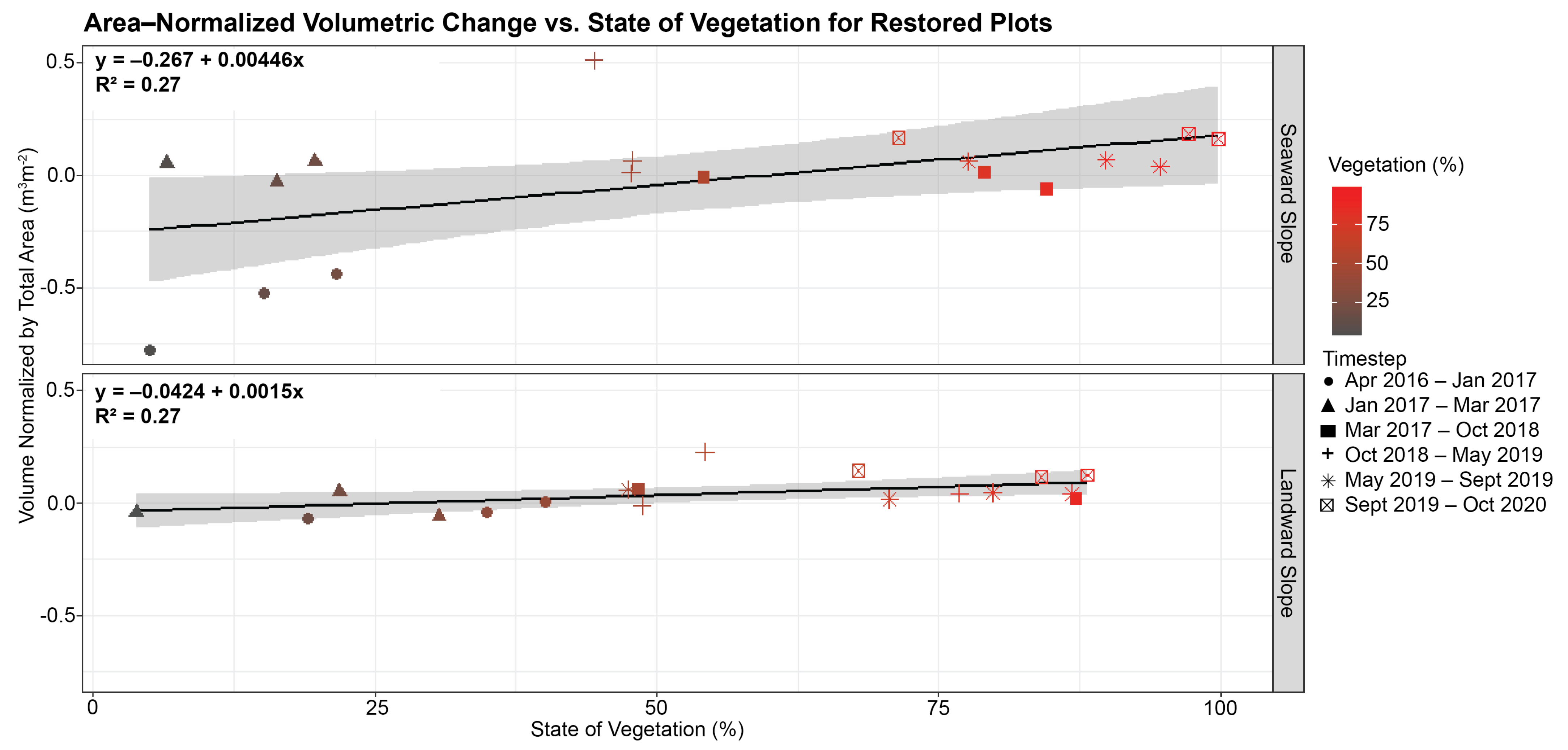
4.4. Vegetation and Geomorphic Change

Changes in vegetation cover and density were calculated through manual digitization and used to inform on potential impacts of vegetation on volumetric changes within the different treatment plots (Section 3.5; Figure 8;

Table 5. E. mollis plant count per m² and percent of dune mat coverage per plot for the restored foredune plots. The beach geomorphic unit was excluded from these calculations because it was not the focus of any replanting efforts. Conditions across the AMM and CON plots were consistent across the study.

Vegetation	Plot	Apr 2016	Jan 2017	Mar 2017	Oct 2017	Oct 2018	May 2019	Sep 2019	Oct 2020
EM per m2	EM	0	0.49	0.38	0.31	0.40	1.01	0.88	0.63
	DM	0	0.02	0.02	0.00	0.02	0.01	0.04	0.02
	DM-EM	0	0.07	0.09	0.05	0.19	0.44	0.34	0.28
DM (% Total Area)	EM	6.95	4.13	4.06	10.05	14.01	18.90	18.54	17.59
	DM	2.06	0.31	0.11	14.50	17.61	23.57	23.49	23.14
	DM-EM	8.53	0.43	0.49	21.64	22.95	29.90	30.24	31.44

). Corresponding erosion and deposition values were provided from the GCD analyses as area-normalized volumetric change (Figure 8).

4.4.1. Changes in Vegetation Coverage

The April 2016 surface reflected the initial removal of invasive plants and, as such, provided a pre-native replanting baseline for assessing changes in vegetation cover. At this time, there were no E. mollis plants and dune mat coverage extended across only 6% the entire domain of foredune identified for restoration (Table 5). January 2017 and March 2017 surfaces represent a post-native replanting and pre-growth stage, during which most of the native species had been planted in the treatment plots, with the exception of some dune mat planting that would occur later in the year. E. mollis planting resulted in a plot density of 0.49 plants per m² in January 2017, decreasing to 0.38 plants per m² by March. By the end of the first growing season (October 2017), E. mollis plot density had continued to decrease, but dune mat planting and natural propagation led to widespread growth, with the highest coverage in the DM-EM plot (21.6%) (Table 5).

Species have generally expanded in cover and density over the three years following the end of the first growing season (2017). E. mollis and dune mat both experienced consistent growth and expansion over the second, third, and fourth growing seasons, despite apparent decreases in E. mollis plants per m² and percent coverage of dune mat (Table 5). These decreases correspond to increases in the total area of the foredune, through seaward and landward extension of the dune, rather than to decreases in the count or coverage of the native species. By the end of the second growing season, some E. mollis had naturally propagated across (<5 m) the north and south edges of the DM plot and densities were up in all treatment plots. The third (2019) and fourth (2020) growing seasons recorded substantial increases in E. mollis in both the EM and DM-EM plots. Dune mat naturally propagated across much of the EM plot, migrating seaward of the foredune crest and spreading across much of the seaward slope by the October 2020 survey (visible in the October 2020 ground photo in Figure 3).

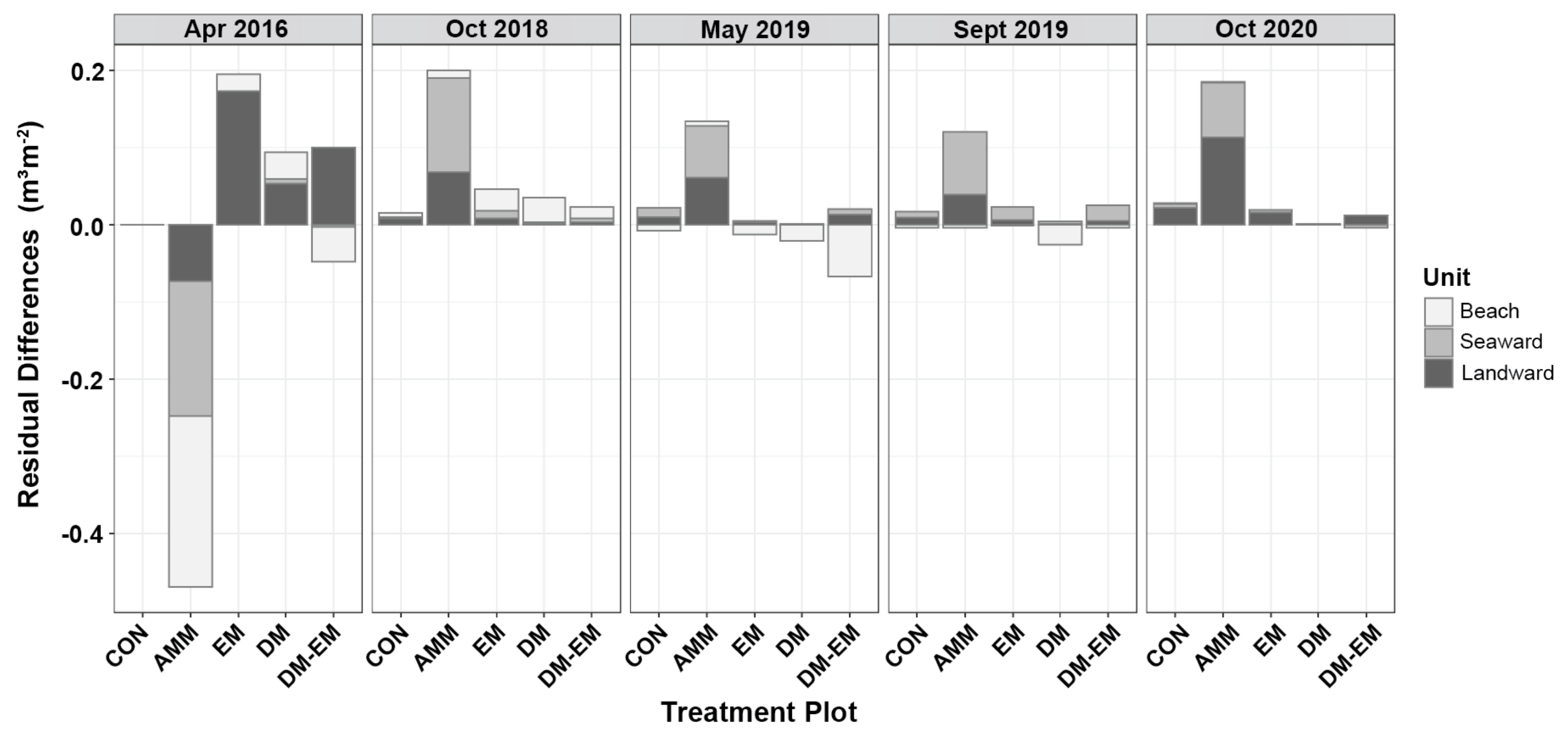
4.4.2. Geomorphic Change Within Vegetation Plots

Subsets of the GCD analyses at Lanphere were divided into the three geomorphic units (beach, seaward slope, landward slope) and five vegetation plots (CON, AMM, EM, DM, DM-EM), resulting in fifteen subset plots. April 2016 did not include the CON plot, because the KAP flight did not extend far enough south to fully encompass the plot or remove edge effects. The growing season prior to planting of the treatment plots (April 2016–January 2017) experienced consistent erosion across most plots and geomorphic units (Figure 8; Table 3).

Minor erosion was recorded in the January–March 2017 interval, related to winter erosive events and a lack of vegetation to hinder transport. By the end of the second growing season (October 2018), the scarp left by erosion during the winter of 2016–2017 had been rebuilt, thereby reconnecting the seaward slope of the foredune with the upper beach in all plots except the AMM plot dominated by A. arenaria (Figure 8 Panel C). Seaward slope accretion was most prominent in the EM plot, with 0.51 m ± 0.03 m of increase observed (Table 3). Erosion between October 2018–May 2019 was consistent across the seaward slope of most treatment plots, following minor scarping of the seaward toe. The seaward toe had reconnected to the upper beach by the September 2019 collection, with accretion recorded on the seaward and landward slopes of all vegetation plots. During the final interval (September 2020–October 2020), all natively vegetated plots recorded between 0.14–0.18 ± 0.03 m and 0.12–0.14 ± 0.04 m of accretion on the seaward and landward slopes of the dune, respectively (Figure 8 Panel F). The seaward slope of the AMM plot, which scarped during the winter storms of 2016–2017, had mostly reconnected with the upper beach by October 2020. An incipient foredune was beginning to form on the upper beach by October 2020, with Cakile edentula (American searocket) and some E. mollis present. Over the entire study, replanted plots recorded erosion of the seaward slope (−0.11 m to −0.21 m ± 0.03) and accretion on the landward slope (0.15–0.32 ± 0.03 m).

A linear regression model was developed to characterize the relationship between sediment erosion and deposition observations and vegetation treatment type. The model shows a weak (R² = 0.27) positive correlation between the state of vegetation (% relative to the local plot maximums) and normalized volumes (m³ m⁻²) for both the seaward and landward slope of the foredune (Figure 10). A positive correlation between area-normalized volume and the state of vegetation suggests that, as the proportion of vegetation within a plot increases, relative to the maximum observed vegetation in that plot, so too does the amount of deposition. There is also a general positive trend over time, such that as vegetation increases, more sediment deposition is observed.

Vegetation at the EREP site had not developed to a state where vegetation-driven geomorphic change was measurable. However, the presence of dune mat species through restoration and natural succession was noted in recent field campaigns during September 2019 and October 2020. The impacts of these plants were not within the range of significantly measurable change in the GCD results, but could serve as loci for future growth and expansion of plant cover. Dune mat plants are visible in the October 2020 orthomosaic and oblique aerial image panels in Figure 4. A. arenaria is present on either side of the rebuilt foredune and is also widespread elsewhere along the south spit of the ELC. No efforts to control A. arenaria have been applied to the area surrounding the rebuilt foredune and future encroachment could further impact biogeomorphic relationships at the EREP site.

5. Discussion

5.1. Cross-Platform Comparison

5.1.1. Variability Between KAP and TLS Methods

We compared the products of our KAP- and UAS-SfM datasets to concurrently collected TLS data (Section 4.2). Two of the removed KAP-SfM datasets (September 2016 and October 2017) exhibited similar issues that arose during processing: high pitch, yaw, and roll variability and a trend in unintentional off-nadir imagery. Imagery from the September 2016 collection had a consistent northerly pitch, which led to increasing diffusivity in the point cloud towards the north, despite thorough manual masking to remove water, the horizon, and distant points from the sparse and dense clouds. Imagery from October 2017 had a consistent southerly pitch and easterly roll, which led to a lack of points in the landward slope and few retained points in the upper beach and seaward slope. The April 2016 KAP-SfM data, despite being successfully aligned to the TLS surface, exhibited the highest vertical error (±0.072 m) across all datasets, as well as the highest variability against the TLS surface. The April KAP-SfM surface also struggled to reconstruct the flat, homogeneous beach, leading to the presence of artifacts and errant surfaces when compared to the TLS surface (Figure 11).

5.1.2. Variability Between UAS and TLS Methods

Our UAS-TLS comparisons featured lower residuals than the KAP-TLS comparison, however there were still consistent differences between the two platforms (Figure 12). Similar to findings by Mancini et al. [8], Guisado-Pintado et al. [32], and Rotnicka et al. [81], our comparison found that the locations of highest variability were located within the beach unit, particularly where wet and relatively featureless sand was present, as well as in areas of dense vegetation, particularly in the AMM plot. We also note that two of the highest residuals were across the seaward slope of the foredune and corresponded with spring acquisition campaigns when the seaward slope was scarped, suggesting that, as discussed by James et al. [79], topographic complexity played a role in limiting the number of convergent points for surface reconstruction on steep slopes. To better highlight the impact of the denser vegetation typical in the AMM and CON plots, we included a summation of UAS-TLS residuals for only the restored plots (EM, DM, DM-EM), where vegetation density was less pronounced. When only the restored plots were compared, residual values across almost all comparisons between the TLS and UAS-SfM residuals were reduced by nearly half (Table 2). When comparing differences between the UAS platforms and concurrent TLS reference surfaces, quality differences were also readily apparent. To fully assess these differences, it helps to consider the state of the final SfM products with concurrent TLS collections. The CON, EM, and DM-EM plots exhibited similar residuals, while the DM plot consistently had the lowest variability, suggesting that sparser, taller grasses may have been impacting the point cloud, even after efforts to remove vegetation (Figure 13).

5.2. UAS for Assessing Geomorphic Change in Restored Coastal Dune Landscapes

This study examines the application of a multi-platform (KAP- and UAS-SfM) approach to detect and interpret sediment erosion and deposition patterns and related geomorphic changes across two beach-dune systems that were the focus of restoration efforts between 2016–2020. A dynamic restoration approach was taken at the Lanphere Dunes to re-establish natural processes within the system through native revegetation and enhancing the potential for aeolian activity. The EREP study site required the reconstruction of a foredune that had experienced a high water breaching event. For the purposes of assessing performance and effectiveness for detecting and quantifying geomorphic change, we used three different aerial platforms referenced to ground-based TLS reference surfaces at our Lanphere study site and two platforms at our EREP study site.

Regional trends in shoreline response, sediment budgets, vegetation cover, and historic foredune evolution and morphodynamics by Rader et al. [27] and Pickart and Hesp [28] provide broader scale context on natural cycles of erosion and deposition and impacts of climatic variability events at the study site. For instance, a north-south trend in sediment availability and shoreline change rates indicate that shoreline progradation and foredune stability are the dominant trends at the Lanphere study site. Despite notable erosion in recent years, foredune recovery via scarp rebuilding to re-establish sand transport from the beach to the foredune is rapid and recent (2000–2016) shoreline and foredune positions have remained relatively stable. Pickart and Hesp [28] also identified a decrease in stabilized forest vegetation and a concurrent increase in herbaceous/scrub vegetation that correlates with a decrease in dune migration rates in observed areas of the North Spit of the ELC, including the Lanphere site. The South Spit of the ELC has not been studied in as much detail, but trends in shoreline change exhibit similar north-south variability [82]. North of the Eel River estuary, shorelines exhibit higher rates of progradation (+1.39 m⁻¹). However, south the estuary, where the EREP site is located, shoreline retreat (−0.24 m⁻¹) and dune erosion are predominant. Considering the observed historical differences in land use, land cover, ownership/management and geomorphology, the Lanphere and EREP study sites are fundamentally different systems - the former is more stable or progradational with stable foredunes, the latter is erosional and with much narrower foredunes. As such, restoration efforts at each site are specific to local conditions and land management strategies.

The Lanphere site required different considerations for characterizing changes in vegetation and in geomorphic change than at the EREP site. While the EREP site was primarily unvegetated, and surface reconstruction was not impacted by the presence of vegetation, the Lanphere site utilized both the high resolution (<0.02 m) orthomosaic imageries, to quantify dune mat and even locate individual E. mollis plants, and the DSM, to quantify surface change. We applied these methods to effectively characterize seasonal changes in vegetation and compare them to seasonal changes in sediment deposition and erosion (Figure 10). However, while the SfM outputs were able to capture erosion and slumping of the seaward toe of the foredune on the upper beach, it generally failed to accurately model the “bare earth” surface of the densely vegetated AMM plot, introducing inaccuracies in the GCD results, as reflected in generally positive residuals when referenced to the coincident TLS baseline datasets. In the restored plots, the impact of vegetation on the change detection results is most pronounced where E. mollis is present. E. mollis, a taller (<1 m) grass, is poorly reconstructed in the SfM point cloud. Rather than a discrete taller feature, the grass is often rendered as a low-lying mound (Figure 13) and is not captured by the vegetation filters applied to strip vegetation from the point clouds. However, considering the magnitude of deviations from the TLS surfaces in the restored plots across all KAP- (<0.06 ± 0.07 m) and UAS-TLS (<0.02 ± 0.03 m) comparisons, we were confident that we effectively captured trends in sediment erosion and deposition and the associated geomorphic responses within the landform units at Lanphere.

While examples of high variance from the TLS reference surfaces were noted in the UAS collections (Section 5.1), these were typically restricted to areas of dense vegetation where, due to a fundamental lack of visibility of the ground surface, both the SfM reconstruction and TLS elevation model struggled to accurately reconstruct a bare earth surface. Higher wind conditions and inconsistencies during collections, such as coverage extent, variable flight altitude, and variable image overlap, proved the biggest downfall across the six KAP datasets (Table 1). Such inconsistencies are driven by a lack of control during KAP data collection. Whereas the UAS collection campaigns employed preprogrammed, automated flight plans that standardized altitude, flight speeds, and regular image overlap, the KAP collection campaigns were driven by external factors, such as winds that drove the gliding altitude or the pace of the person walking the kite. As outlined by James et al. [31] and Singh and Frazier [4], consistency is essential for quality SfM processing, representing a flaw inherent to the use of KAP datasets for surface modeling and topographic differencing. While we agree with Duffy et al. [33] that KAP provides a low-cost, highly portable, easy to deploy and maintain technique for aerial mapping, careful consideration should be taken to standardize repeat-collection methods if topographic differencing is a desired product. Methods to improve KAP-SfM efficiency and increase point confidence in complex terrains could include decreasing the distance between walking passes to increase image overlap, including off-nadir imagery to improve convergent angle feature reconstruction [4,83], or choosing a kite suitable for wind conditions to improve flight stability. Such techniques, regularly used to improve consistency in UAS-SfM point clouds [4], would work well to improve KAP-SfM point clouds.

5.3. Uncertainty Budget Calculation

The detection and quantification of topographic change, using DEMs or DSMs derived from close-range remote sensing platforms, requires many subjective decisions that include sensor choice, flight parameters and acquisition planning, georeferencing and geocorrection methods, processing parameters, and post-processing comparison techniques. Each of the items listed above represent choices that are made by both the pilot and field crew who collect the data, as well as the analyst(s) who process the data and develop the DEMs. When developing an uncertainty budget, each of these choices implies a possible deviation in methodology across surveys or analysts. Our uncertainty budgets for each unique acquisition campaign incorporated GCP error (for the quadcopter UAS and KAP surveys) or total XYZ error (for the fixed-wing UAS surveys), RTK accuracy (both for georeferencing of GCPs and for the fixed-wing UAS with onboard RTK), and RMSE generated from the alignment of the point clouds to a reference point cloud (e.g., TLS point clouds at the Lanphere site, geocorrected May 2018 point cloud at the EREP site).

In developing our uncertainty budget, we assumed that uncertainty would be introduced from a combination of collection and processing methods and that: (1) the uncertainty can be represented by a global, or uniform model (vs. spatially variable), (2) the accuracy of data from the aerial platforms can be assessed by alignment and comparison to concurrently collected TLS data, (3) that KAP- and UAS-SfM products are comparable when processed with consistent methodology, and (4) that the delineation of geomorphic units and vegetation treatment types is useful for identifying and interpreting the performance of the aerial platforms for detecting change. Others, such as Duffy et al. [33] and Guisado-Pintado et al. [32], calculated their budget using reported RMS errors. Wheaton et al. [45] discussed a more encompassing uncertainty budget approach that could include manufacturer reported equipment precision, measurement error, sampling bias, interpolation methods, differences from repeat occupation of a control point, and spatial variability. Bangen et al. [84] built on that and discussed uncertainty budget development and error propagation, suggesting that error could be introduced by survey methods, sampling strategy, and surface complexity. In the context of the coastal zone, variability and possible sources of uncertainty could even extend to weather, tidal, and moisture conditions or seasonal variability in the complexity of the terrain or vegetation cover [32,81].

While we found examples of study-specific uncertainty budgets, e.g., [32,45,84], we were unable to find a standardized budget construction method that allows uncertainty to be compared across different studies. Our calculated error totals (Table 1) were similar in magnitude to those used by Guisado-Pintado et al. [32], although we came to our values in a completely different way. This highlights a shortcoming in the current discussion and understanding of propagated error in the method of topographic differencing and geomorphic change detection. While many [31,38,45,69,73,84,85,86] have discussed uncertainty and how to calculate propagated error for topographic differencing, we were unable to find a consensus amongst publications in the geodesy or geoscience communities that aimed to standardize the ways in which a budget is constructed, what should be included, or to what extent possible sources are attributable. Standardization and community-developed guidelines could reduce the subjectivity inherent in creating an uncertainty budget, improve cross-study comparability, and strengthen methods for reproducibility and replicability of UAS-SfM studies across the geosciences. Photogrammetric software, like Agisoft Metashape, and federally managed geocorrection services, like the NOAA-operated OPUS, include various forms of reported error and uncertainty that can be used in SfM processing and geocorrectional accuracy. Equipment manufacturers can also provide precision and accuracy expectations with their products, though this is not standard practice, and varies between companies. Point cloud processing software, such as the open-source program CloudCompare (https://www.danielgm.net/cc/), provide alignment RMSE when aligning point clouds. While these are only some examples of reported uncertainty, consideration and inclusion of similar products will improve the reasonable minimum level of detection when calculating topographic differences.

It is helpful to revisit the two previously mentioned (Section 3.3) sources of uncertainty that we considered for geomorphic SfM-related work: (1) collection uncertainty and (2) processing uncertainty. Collection uncertainty could include equipment precision, measurement error, sampling bias/strategy, variations in the repeat occupation of a survey point, or survey method differences, to name a few. These deviations inflate uncertainty by decreasing the likelihood that a surface was accurately located in space and increasing the minimum level of detection for topographic differencing. If not properly accounted for or considered, these sources of uncertainty can propagate and impact the accuracy of volumetric difference calculations, or overestimate the significance threshold, removing unnecessary raster cells from the output model. The KAP-SfM datasets provide an example of a dataset driven by heightened collection uncertainty. For these datasets, the processing procedure was consistent with all other UAS-SfM datasets, however collection methods were highly variable, with differences in site extent, image overlap, flight altitude, and external (wind speed and direction) factors playing a role in inflating uncertainty or rendering a dataset unusable. The UAS-SfM datasets exhibited less than half of the uncertainty reported by the April 2016 KAP-SfM dataset. More comprehensive methods for controlling and standardizing flight plans, image overlap, and altitude, as well as more rigorous geocorrection strategies, led to lower collection uncertainties across the four UAS-SfM datasets. Based on our experiences, we found that standardization was a major driver for accurate and confident surface reconstruction, explaining why the pre-programmed UAS-SfM datasets were far less problematic than the KAP-SfM datasets.

Processing uncertainty is driven by decisions during the creation of the SfM dataset within virtual space, including parameter choices, the filtering of low confidence points, manual point cloud cleaning efforts, or the accuracy of the point cloud-to-point cloud alignment process. These variables have the potential to be more subjective and can be based on the processing time that an analyst is willing to spend preparing and refining a dataset. Processing uncertainty in our study was primarily driven by point cloud alignment. Similar to the factors contributing to collection uncertainty, our processing uncertainty was inflated in the KAP-SfM datasets because of how lower point confidence translated to the removal of more points throughout the point cloud and to higher RMSE during the SfM to TLS alignment step. The UAS-SfM datasets featured lower alignment RMSE than the KAP-SfM datasets, but still exhibited residual artifacts where vegetation was present, even following filtering and manual point cloud cleaning efforts. A downfall of automated classification methods used in our research, that could have contributed to the inability to detect the vegetation signature, stemmed from seasonal vegetation phenology and the color of vegetation during the collection campaigns. Our collections occurred in early spring, before much new plant growth had occurred, and in fall, as vegetation was starting to senesce. Vegetation color was often a light brown during our collection campaigns, which became muddled with the color of the surrounding sand, making automatic classification more difficult and increasing uncertainty within the point clouds.

We propose that, when constructing uncertainty budgets for topographic differencing, one considers and compounds the primary sources of collection uncertainty (e.g., equipment precision, flight conditions) and processing uncertainty (e.g., point cloud alignment RMSE, overall GCP or total image error) inherent to their data. Flight conditions (e.g., wind speed and direction, lighting) and collection parameters (altitude, image overlap, capture angle) should also be reported, to better describe external factors that could impact SfM products. Employing this practice requires careful consideration of the possible influences on a KAP or UAS campaign, and subsequent processing procedures, and can better contextualize the range of impacts on uncertainty that is possible throughout the process. Including unique, campaign-specific uncertainty will not only improve reporting procedures and comparability between datasets, but will also help convey the range of values that may not be realistically measurable when reporting the results of topographic differencing. Finally, we realize that developing a standardized method for uncertainty budgeting requires comprehensive knowledge of the possible influences on an SfM dataset and that it can be a difficult task to undertake, particularly with the rapid development of new technologies and methods. A broader commentary on the equipment, procedures, and decisions made during SfM data collection and processing, and how those factors impact uncertainty, would greatly serve the geoscience and geodesy communities and further the development of standard, reproducible, and replicable procedures, much like those suggested by James et al. [31].

6. Conclusions

We have highlighted necessary considerations when attempting to employ and reconcile multiple aerial platforms for assessing geomorphic change detection related to changes in vegetation in restored coastal dune landscapes. Our two study areas in the Lanphere Dunes and Eel River Estuary Preserve in northern California present two very different examples of restored ecosystems with very different goals. Dynamic restoration of the foredune at Lanphere focused on restoring naturally-driven foredune resiliency through native revegetation. We used the GCD toolset in ArcMap 10.7.1 to quantify sediment erosion and deposition between collection intervals and related those changes to the different treatment plots. We found that our multi-platform approach captured significant geomorphic change across all geomorphic units and treatment plots, though the residual impact of vegetation led to a potential overestimation of change volumes. Restoration at the EREP site involved foredune reconstruction that aimed at repairing the natural foredune barrier to preserve landward interests. At EREP, we were able to quantify significant change across the foredune from its initial construction (summer 2018) through October 2020. Geomorphic change at the EREP site was not driven by the presence of vegetation and, because of this, volumetric differences were not dependent on the accuracy of spurious (vegetation) point removal. We feel that our approach contextualized change at each location and showed that a multi-platform approach can effectively characterize sediment erosion and deposition, as well as vegetation change in restored coastal foredune ecosystems. Finally, we propose the inclusion of two primary forms of uncertainty, collection and processing uncertainty, when utilizing KAP- or UAS-SfM products for topographic differencing. Employing this approach requires careful consideration of where uncertainty arises within an SfM dataset and how that uncertainty propagates throughout the dataset. Incorporating multiple levels of uncertainty (e.g., level of GNSS accuracy, total XYZ error, point cloud-point cloud alignment) allows for a better understanding of realistic change within a topographic difference interval and can be a standardized method to compare uncertainty across datasets and in the broader discipline. Our main findings are:

• Geomorphic change detection, coupled with SfM datasets, is a valuable tool for geomorphologists and land managers to characterize statistically significant changes in geomorphic systems and, as we have shown, restored systems. However, when using conventional SfM it is necessary to consider the impacts that vegetation, moisture, and topographic complexity may have on reconstruction accuracy and point confidence. Failure to consider these factors may result in the exaggeration of differences between intervals and/or platforms.
• When compared to TLS datasets with better constraints on vegetation removal, the aerial datasets performed well, but struggled in areas of denser vegetation. Even after efforts to remove vegetation from the constructed dense point cloud, artifacts were still apparent when comparing concurrently collected surfaces. The UAS data struggled to accurately capture true geomorphic change in areas of dense vegetation, but deviations from the TLS datasets were typically on the order of 15% of the total area and 0.01–0.02 m of area-normalized volumetric difference (m³m⁻²).
• Uncertainty budgets for aerial datasets require careful consideration of the possible avenues for introducing error. This is further complicated by a lack of standardization or suggested best practices for constructing an uncertainty budget. We viewed inputs in terms of collection and processing uncertainty and our budgets reflected the sum of those inputs. However, the variety of uncertainty budgets for geomorphic change across published research highlights a need for more standard practices.

We suggest that future efforts in the geoscience and geodesy communities focus on standardizing methodology for SfM processing, similar to the methods proposed by James et al. [31]. Standardization of these methods should also focus on the impact that collection- and processing-based uncertainty have on SfM products. Efforts to improve these methods will not only improve transparency and reporting practices, but would also hold the rapidly advancing field of SfM photogrammetry for topographic differencing more accountable for the decisions made during processing and analysis of results. For coastal geomorphologist and resource managers, it is imperative that reported results accurately and reasonably describe sediment budgets and geomorphic change to better prepare for the widespread impact that increased coastal flooding and erosion will have on communities living along the coast.

References

1. Westoby, M.J.; Brasington, J.; Glasser, N.; Hambrey, M.; Reynolds, J.M. ‘Structure-from-Motion’ photogrammetry: A low-cost, effective tool for geoscience applications. Geomorphology 2012, 179, 300–314. [Google Scholar] [CrossRef] [Green Version]
2. Fonstad, M.; Dietrich, J.; Courville, B.; Jensen, J.; Carbonneau, P. Topographic structure from motion: a new development in photogrammetric measurement. Earth Surf. Proc. Land. 2013, 38, 421–430. [Google Scholar] [CrossRef] [Green Version]
3. Smith, M.W.; Carrivick, J.; Quincey, D. Structure from motion photogrammetry in physical geography. Prog. Phys. Geog. 2016, 40, 247–275. [Google Scholar] [CrossRef] [Green Version]
4. Singh, K.K.; Frazier, A.E. A meta-analysis and review of unmanned aircraft system (UAS) imagery for terrestrial applications. Int. J. Remote Sens. 2018, 39, 5078–5098. [Google Scholar] [CrossRef]
5. Anderson, K.; Westoby, M.; James, M. Low-budget topographic surveying comes of age: Structure from motion photogrammetry in geography and the geosciences. Prog. Phys. Geogr. 2019, 43, 163–173. [Google Scholar] [CrossRef]
6. Fonstad, M.; Zettler-Mann, A. The camera and the geomorphologist. Geomorphology 2020, 366, 107181. [Google Scholar] [CrossRef]
7. Delgado-Fernandez, I.; Davidson-Arnott, R.; Ollerhead, J. Application of a Remote Sensing Technique to the Study of Coastal Dunes. J. Coast. Res. 2009, 2009, 1160–1167. [Google Scholar] [CrossRef]
8. Mancini, F.; Dubbini, M.; Gattelli, M.; Stecchi, F.; Fabbri, S.; Gabbianelli, G. Using Unmanned Aerial Vehicles (UAV) for High-Resolution Reconstruction of Topography: The Structure from Motion Approach on Coastal Environments. Remote Sens. 2013, 5, 6880–6898. [Google Scholar] [CrossRef] [Green Version]
9. Turner, I.L.; Harley, M.D.; Drummond, C.D. UAVs for coastal surveying. Coast. Eng. 2016, 114, 19–24. [Google Scholar] [CrossRef]
10. Sturdivant, E.; Lentz, E.; Thieler, E.R.; Farris, A.; Weber, K.; Remsen, D.; Miner, S.; Henderson, R. UAS-SfM for Coastal Research: Geomorphic Feature Extraction and Land Cover Classification from High-Resolution Elevation and Optical Imagery. Remote Sens. 2017, 9, 1020. [Google Scholar] [CrossRef] [Green Version]
11. Hodgson, M.E.; Morgan, G.R. Modeling Sensitivity of Topographic Change with sUAS Imagery. Geomorphology 2020, 8, 107563. [Google Scholar] [CrossRef]
12. Luijendijk, A.; Hagenaars, G.; Ranasinghe, R.; Baart, F.; Donchyts, G.; Aarninkhof, S. The State of the World’s Beaches. Sci. Rep. 2018, 8, 6641. [Google Scholar] [CrossRef] [PubMed]
13. Luijendijk, A.; de Vries, S. Global beach database. In Sandy Beach Morphodynamics; Elsevier: Amsterdam, The Netherlands, 2020; Chapter 26; pp. 641–658. [Google Scholar] [CrossRef]
14. National Academies of Sciences Engineering and Medicine. A Vision for NSF Earth Sciences 2020–2030; National Academies Press: Washington, DC, USA, 2020. [Google Scholar]
15. Nordstrom, K.F. Beaches and dunes of human-altered coasts. Prog. Phys. Geog. 1994, 18, 497–516. [Google Scholar] [CrossRef]
16. Gangaiya, P.; Beardsmore, A.; Miskiewicz, T. Morphological changes following vegetation removal and foredune re-profiling at Woonona Beach, New South Wales, Australia. Ocean Coast. Manag. 2017, 146, 15–25. [Google Scholar] [CrossRef]
17. Ketchum, B.H. The Water’s Edge: Critical Problems of the Coastal Zone; MIT Press: Cambridge, MA, USA, 1972. [Google Scholar]
18. Martínez, M.L.; Hesp, P.A.; Gallego-Fernández, J.B. Coastal Dunes: Human Impact and Need for Restoration. In Restoration of Coastal Dunes; Martinez, M.L., Gallego-Fernandez, J.B., Hesp, P.A., Eds.; Springer: Berlin, Germany, 2013; Chapter 1; pp. 1–14. [Google Scholar] [CrossRef]
19. Everard, M.; Jones, L.; Watts, B. Have we neglected the societal importance of sand dunes? An ecosystem services perspective. Aquat. Conserv. 2010, 20, 476–487. [Google Scholar] [CrossRef]
20. Hesp, P.A. Foredunes and blowouts: Initiation, geomorphology and dynamics. Geomorphology 2002, 48, 245–268. [Google Scholar] [CrossRef]
21. Walker, I.J.; Davidson-Arnott, R.G.D.; Bauer, B.O.; Hesp, P.A.; Delgado-Fernandez, I.; Ollerhead, J.; Smyth, T.A.G. Scale-dependent perspectives on the geomorphology and evolution of beach-dune systems. Earth Sci. Rev. 2017, 171, 220–253. [Google Scholar] [CrossRef]
22. Hesp, P.A.; Walker, I.J. 11.17 Coastal Dunes. In Treatise on Geomorphology; Shroder, J.F., Ed.; Elsevier: Amsterdam, The Netherlands, 2013; Volume 11, Chapter 11.17; pp. 328–355. [Google Scholar]
23. Martínez, M.L.; Gallego-Fernández, J.B.; Hesp, P.A. (Eds.) Restoration of Coastal Dunes; Springer Series on Environmental Management; Springer: Berlin/Heidelberg, Germany, 2013. [Google Scholar] [CrossRef]
24. Ollerhead, J.; Davidson-Arnott, R.G.D.; Walker, I.J.; Mathew, S. Annual to decadal morphodynamics of the foredune system at Greenwich Dunes, Prince Edward Island, Canada. Earth Surf. Process. Landforms 2013, 38, 284–298. [Google Scholar] [CrossRef]
25. Pickart, A.; Sawyer, J. Ecology and Restoration of Northern California Coastal Dunes; California Native Plant Society: Sacramento, CA, USA, 1998. [Google Scholar]
26. Barnard, P.; Short, A.; Harley, M.; Splinter, K.; Vitousek, S.; Turner, I.; Allan, J.; Banno, M.; Bryan, K.; Doria, A.; et al. Coastal vulnerability across the Pacific dominated by El Niño/Southern Oscillation. Nat. Geosci. 2015, 8, 801–807. [Google Scholar] [CrossRef]
27. Rader, A.M.; Pickart, A.J.; Walker, I.J.; Hesp, P.A.; Bauer, B.O. Foredune morphodynamics and sediment budgets at seasonal to decadal scales: Humboldt Bay National Wildlife Refuge, California, USA. Geomorphology 2018, 318, 69–87. [Google Scholar] [CrossRef]
28. Pickart, A.J.; Hesp, P.A. Spatio-temporal geomorphological and ecological evolution of a transgressive dunefield system, Northern California, USA. Glob. Planet. Chang. 2019, 172, 88–103. [Google Scholar] [CrossRef]
29. Walker, I.J.; Hesp, P.A. 11.7 Fundamentals of Aeolian Sediment Transport: Airflow Over Dunes. In Treatise on Geomorphology; Shroder, J.F., Ed.; Elsevier: Amsterdam, The Netherlands, 2013; Volume 11, Chapter 11.7; pp. 109–133. [Google Scholar]
30. Yager, E.M.; Schmeeckle, M.W. The influence of vegetation on turbulence and bed load transport. J. Geophys. Res. Earth Surf. 2013, 118, 1585–1601. [Google Scholar] [CrossRef]
31. James, M.R.; Chandler, J.H.; Eltner, A.; Fraser, C.; Miller, P.E.; Mills, J.P.; Noble, T.; Robson, S.; Lane, S.N. Guidelines on the use of structure-from-motion photogrammetry in geomorphic research. Earth Surf. Process. Landforms 2019, 44, 2081–2084. [Google Scholar] [CrossRef]
32. Guisado-Pintado, E.; Jackson, D.W.T.; Rogers, D. 3D mapping efficacy of a drone and terrestrial laser scanner over a temperate beach-dune zone. Geomorphology 2019, 328, 157–172. [Google Scholar] [CrossRef]
33. Duffy, J.; Shutler, J.; Witt, M.; DeBell, L.; Anderson, K. Tracking Fine-Scale Structural Changes in Coastal Dune Morphology Using Kite Aerial Photography and Uncertainty-Assessed Structure-from-Motion Photogrammetry. Remote Sens. 2018, 10, 1494. [Google Scholar] [CrossRef] [Green Version]
34. Madurapperuma, B.; Close, P.; Fleming, S.; Collin, M.; Thuresson, K.; Lamping, J.; Dellysse, J.; Cortenbach, J. Habitat Mapping of Ma-le’l Dunes Coupling with UAV and NAIP Imagery. Proceedings 2018, 2, 368. [Google Scholar] [CrossRef] [Green Version]
35. Madurapperuma, B.; Lamping, J.; McDermott, M.; Murphy, B.; McFarland, J.; Deyoung, K.; Smith, C.; MacAdam, S.; Monroe, S.; Corro, L.; et al. Factors Influencing Movement of the Manila Dunes and Its Impact on Establishing Non-Native Species. Remote Sens. 2020, 12, 1536. [Google Scholar] [CrossRef]
36. Van Puijenbroek, M.E.B.; Nolet, C.; de Groot, A.V.; Suomalainen, J.M.; Riksen, M.J.P.M.; Berendse, F.; Limpens, J. Exploring the contributions of vegetation and dune size to early dune development using unmanned aerial vehicle (UAV) imaging. Biogeosciences 2017, 14, 5533–5549. [Google Scholar] [CrossRef] [Green Version]
37. Nolet, C.; van Puijenbroek, M.E.B.; Suomalainen, J.M.; Limpens, J.; Riksen, M.J.P.M. UAV-imaging to model growth response of marram grass to sand burial: Implications for coastal dune development. Aeolian Res. 2018, 31, 50–61. [Google Scholar] [CrossRef]
38. Eamer, J.; Walker, I. Quantifying spatial and temporal trends in beach-dune volumetric changes using spatial statistics. Geomorphology 2013, 191, 94–108. [Google Scholar] [CrossRef]
39. Walker, I.J.; Eamer, J.B.R.; Darke, I.B. Assessing significant geomorphic changes and effectiveness of dynamic restoration in a coastal dune ecosystem. Geomorphology 2013, 199, 192–204. [Google Scholar] [CrossRef]
40. Darke, I.; Eamer, J.; Beaugrand, H.; Walker, I. Monitoring considerations for a dynamic dune restoration project: Pacific Rim National Park Reserve, British Columbia, Canada. Earth Surf. Proc. Land. 2013, 38, 983–993. [Google Scholar] [CrossRef]
41. Scarelli, F.M.; Sistilli, F.; Fabbri, S.; Cantelli, L.; Barboza, E.G.; Gabbianelli, G. Seasonal dune and beach monitoring using photogrammetry from UAV surveys to apply in the ICZM on the Ravenna coast (Emilia-Romagna, Italy). Remote Sens. Appl. Soc. Environ. 2017, 7, 27–39. [Google Scholar] [CrossRef]
42. Ruessink, B.G.; Arens, S.M.; Kuipers, M.; Donker, J.J.A. Coastal dune dynamics in response to excavated foredune notches. Aeolian Res. 2018, 31, 3–17. [Google Scholar] [CrossRef]
43. Costas, S.; de Sousa, L.B.; Kombiadou, K.; Ferreira, Ó.; Plomaritis, T.A. Exploring foredune growth capacity in a coarse sandy beach. Geomorphology 2020, 371, 107435. [Google Scholar] [CrossRef]
44. Riverscapes Consortium. Geomorphic Change Detection 7. 2020. Available online: http://gcd.riverscapes.xyz/ (accessed on 18 June 2020).
45. Wheaton, J.M.; Brasington, J.; Darby, S.E.; Sear, D.A. Accounting for uncertainty in DEMs from repeat topographic surveys: Improved sediment budgets. Earth Surf. Proc. Land. 2010, 35, 136–156. [Google Scholar] [CrossRef]
46. Wheaton, J.M.; Brasington, J.; Darby, S.E.; Merz, J.; Pasternack, G.B.; Sear, D.A.; Vericat, D. Linking geomorphic changes to salmonid habitat at a scale relevant to fish. River Res. Appl. 2010, 26, 469–486. [Google Scholar] [CrossRef]
47. Patsch, K.; Griggs, G.B. Development of Sand Budgets for California’s Major Littoral Cells. Calif. Coast. Rec. Proj. 2007, 1–115. [Google Scholar] [CrossRef]
48. Patton, J.R.; Williams, T.B.; Anderson, J.K.; Leroy, T.H. Tectonic Land Level Changes and Their Contribution to Sea-Level Rise, Humboldt Bay Region, Northern California; Technical Report; Cascadia Geosciences: Arcata, CA, USA, 2017. [Google Scholar]
49. Burgette, R.J.; Weldon, R.J.; Schmidt, D.A. Interseismic uplift rates for western Oregon and along-strike variation in locking on the Cascadia subduction zone. J. Geophys. Res. Solid Earth 2009, 114, 1–24. [Google Scholar] [CrossRef] [Green Version]
50. Patsch, K.; Griggs, G.B. Littoral Cells, Sand Budgets, and Beaches: Understanding California’s Shoreline. In California Department of Boating and Waterways, California Coastal Sediment Management Workgroup; Institute of Marine Sciences, University of California: Santa Cruz, CA, USA, 2006. [Google Scholar]
51. Black, J.; Gress, C.; Byers, J.; Jennings, E.; Ely, C. Behaviour of wintering Tundra Swans Cygnus columbianus columbianus at the Eel River delta and Humboldt Bay, California, USA. Wildfowl 2010, 60, 38–51. [Google Scholar]
52. Monroe, G.; Reynolds, F. Natural Resources of the Eel River Delta; Technical Report; California Department of Fish and Game: Sacramento, CA, USA, 1974. [Google Scholar]
53. Carslaw, D.C.; Ropkins, K. Openair—An R Package for Air Quality DATA analysis. Environ. Model. Softw. 2012, 27–28, 52–61. [Google Scholar] [CrossRef]
54. Carslaw, D.C. The Openair Manual—Open-Source Tools for Analysing Air Pollution Data; Manual for Version 2.6-6. 2019. Available online: https://cran.r-project.org/web/packages/openair/index.html (accessed on 17 December 2020).
55. Pickart, A. Dune Restoration Over Two Decades at the Lanphere and Ma-le’l Dunes in Northern California. In Restoration of Coastal Dunes; Martínez, M., Gallego-Fernández, J., Hesp, P., Eds.; Springer: Berlin/Heidelberg, Germany, 2013; pp. 159–171. [Google Scholar]
56. Buell, A.; Pickart, A.; Stuart, J. Introduction History and Invasion Patterns of Ammophila arenaria on the North Coast of California. Conserv. Biol. 1995, 9, 1587–1593. [Google Scholar] [CrossRef]
57. Tobias, M.M. California foredune plant biogeomorphology. Phys. Geogr. 2015, 36, 19–33. [Google Scholar] [CrossRef]
58. Pickart, A. Control of European Beachgrass (Ammophila arenaria) on the West Coast of the United States; California Exotic Pest Council: Berkeley, CA, USA, 1997; pp. 1–8. [Google Scholar]
59. Costa, S.; Glatzel, K. Humboldt Bay, California, Entrance Channel. Report 1: Data Review; Technical Report; Coastal and Hydraulics Lab, U.S. Army Engineer Research and Development Center: Vicksburg, MS, USA, 2002. [Google Scholar]
60. Hapke, C.J.; Reid, D.; Richmond, B.M.; Ruggiero, P.; List, J. National assessment of shoreline change: Part 3: Historical shoreline changes and associated coastal land loss along the sandy shorelines of the California coast. US Geol. Surv. Open File Rep. 2006, 1219, 79. [Google Scholar]
61. Sallenger, A., Jr. Storm impact scale for barrier islands. J. Coast. Res. 2000, 16, 890–895. [Google Scholar]
62. Houser, C.; Hapke, C.; Hamilton, S. Controls on coastal dune morphology, shoreline erosion and barrier island response to extreme storms. Geomorphology 2008, 100, 223–240. [Google Scholar] [CrossRef]
63. Mathew, S.; Davidson-Arnott, R.; Ollerhead, J. Evolution of a beach–dune system following a catastrophic storm overwash event: Greenwich Dunes, Prince Edward Island, 1936–2005. Can. J. Earth Sci. 2010, 47, 273–290. [Google Scholar] [CrossRef]
64. The Wildlands Conservancy. Eel River Estuary Preserve (EREP) Management Plans; Technical Report; The Wildlands Conservancy: Oak Glen, CA, USA, 2017. [Google Scholar]
65. James, M.; Antoniazza, G.; Robson, S.; Lane, S. Mitigating systematic error in topographic models for geomorphic change detection: Accuracy, precision and considerations beyond off-nadir imagery. Earth Surf. Proc. Land. 2020, 45, 2251–2271. [Google Scholar] [CrossRef]
66. Mosbrucker, A.R.; Major, J.J.; Spicer, K.R.; Pitlick, J. Camera system considerations for geomorphic applications of SfM photogrammetry. Earth Surf. Process. Landforms 2017, 42, 969–986. [Google Scholar] [CrossRef] [Green Version]
67. Agisoft, L.L.C. Agisoft Metashape User Manual: Professional Edition; St. Petersburg, Russia, 2019. [Google Scholar]
68. Bayley, D.T.I.; Mogg, A.O.M. A protocol for the large-scale analysis of reefs using Structure from Motion photogrammetry. Methods Ecol. Evol. 2020, 11. [Google Scholar] [CrossRef]
69. Wernette, P.A.; Lehner, J.; Houser, C. What is ‘real’? Identifying erosion and deposition in context of spatially-variable uncertainty. Geomorphology 2020, 355, 107083. [Google Scholar] [CrossRef]
70. Hon, G. Error: the long neglect, the one-sided view, and a typology. In Going Amiss in Experimental Research; Springer: Berlin, Germany, 2009; pp. 11–26. [Google Scholar]
71. Sherman, D.J. Understanding wind-blown sand: Six vexations. Geomorphology 2020, 366. [Google Scholar] [CrossRef]
72. Brasington, J.; Rumsby, B.T.; Mcvey, R.A. Monitoring and modelling morphological change in a braided gravel-bed river using high resolution GPS-based survey. Earth Surf. Proc. Land. 2000, 25, 973–990. [Google Scholar] [CrossRef]
73. Lane, S.N.; Westaway, R.M.; Hicks, M. Estimation of erosion and deposition volumes in a large, gravel-bed, braided river using synoptic remote sensing. Earth Surf. Proc. Land. 2003, 28, 249–271. [Google Scholar] [CrossRef]
74. Rader, A. Foredune Morphodynamics and Seasonal Sediment Budget Patterns: Humboldt Bay National Wildlife Refuge, Northern California, USA. Master’s Thesis, University of Victoria, Victoria, BC, Canada, 2017. [Google Scholar]
75. Chiba, T.; Kaneta, S.; Suzuki, Y. Red relief image map: New visualization method for three dimensional data. Int. Arch. Photogramm. Remote Sens. Spat. Inf. Sci. 2008, 37, 1071–1076. [Google Scholar]
76. Smith, A.; Houser, C.; Lehner, J.; George, E.; Lunardi, B. Crowd-sourced identification of the beach-dune interface. Geomorphology 2020, 367, 107321. [Google Scholar] [CrossRef]
77. Wickham, H. ggplot2: Elegant Graphics for Data Analysis; Springer: New York, NY, USA, 2016. [Google Scholar]
78. James, M.R.; Robson, S. Mitigating systematic error in topographic models derived from UAV and ground-based image networks. Earth Surf. Proc. Land. 2014, 39, 1413–1420. [Google Scholar] [CrossRef] [Green Version]
79. James, M.R.; Robson, S.; Smith, M.W. 3-D uncertainty-based topographic change detection with structure-from-motion photogrammetry: Precision maps for ground control and directly georeferenced surveys. Earth Surf. Proc. Land. 2017, 42, 1769–1788. [Google Scholar] [CrossRef]
80. Meyer, F.; Perrier, V.; Carroll, I.; Dang, X. Esquisse: Explore and Visualize Your Data Interactively. Available online: https://cran.r-project.org/package=esquisse (accessed on 17 December 2020).
81. Rotnicka, J.; Dłużewski, M.; Da̧bski, M.; Rodzewicz, M.; Włodarski, W.; Zmarz, A. Accuracy of the UAV-Based DEM of Beach–Foredune Topography in Relation to Selected Morphometric Variables, Land Cover, and Multitemporal Sediment Budget. Estuaries Coasts 2020, 43, 1939–1955. [Google Scholar] [CrossRef]
82. GHD. Coastal Dune Vulnerability and Adaptation Study: Eel River Shoreline Trends; GHD: Eureka, CA, USA, 2018. [Google Scholar]
83. Smith, M.W.; Vericat, D. From experimental plots to experimental landscapes: Topography, erosion and deposition in sub-humid badlands from Structure-from-Motion photogrammetry. Earth Surf. Process. Landforms 2015, 40, 1656–1671. [Google Scholar] [CrossRef] [Green Version]
84. Bangen, S.G.; Hensleigh, J.; McHugh, P.; Wheaton, J.M. Error modeling of DEMs from topographic surveys of rivers using fuzzy inference systems. Water Resour. Res. 2016, 52, 1176–1193. [Google Scholar] [CrossRef] [Green Version]
85. Anderson, S. Uncertainty in quantitative analyses of topographic change: error propagation and the role of thresholding. Earth Surf. Proc. Land. 2019, 44, 1015–1033. [Google Scholar] [CrossRef]
86. Griffiths, D.; Burningham, H. Comparison of pre- and self-calibrated camera calibration models for UAS-derived nadir imagery for a SfM application. Prog. Phys. Geog. 2019, 43, 215–235. [Google Scholar] [CrossRef] [Green Version]
Figure 1. Study area map showing the Eureka Littoral Cell, Lanphere Dunes, and Eel River Estuary Preserve (EREP) study sites. The beach and Pacific Ocean are to the west and the foredune is in the center in both callout maps. The two study sites represent typical dune morphology on the South and North Spits of Humboldt Bay. Southern spit dunes are characterized by narrower, reflective beaches without transgressive dune complexes landward. Northern spit dunes are characterized by wider beaches with larger active transgressive dune fields and vegetated relict dunes.
Remotesensing 13 00354 g001
Figure 2. Annual wind rose and annual wave rose generated from 24-hour observation for North Spit, CA and Eureka, CA, respectively. Wind rose data was sourced from NOAA Station HBYC1 (9418767) at North Spit, CA, (40.767 N, 124.217 W). Wave rose data was sourced from NBDC Station 46022 17NM WSW of Eureka, CA (40.703 N, 124.554 W). Wind and wave data were processed using the RStudio package ‘openair’ [53,54].
Remotesensing 13 00354 g002
Figure 3. Map of orthomosaics from the first and last collection at the Lanphere Dunes. The beach and Pacific Ocean are to the west and the foredune is in the center of both callout maps. Plots are labeled as native control (CON), A. arenaria (AMM), E. mollis (EM), dune mat (DM), and mixed dune mat-E. mollis (DM-EM) and represent restoration treatment plots established prior to the January 2017 campaign. The arrows in the October 2020 orthomosaic provide the vantage point, looking NNE, for the three photos to the right. The April 2016 (photo credit: A. Rader) and October 2020 (photo credit: Z. Hilgendorf) photos were taken during data collection. The May 2017 (photo credit: A. Rader) photo was taken shortly after native replanting. Transects A–A’ and A1–A1’ are discussed in Figure 7.
Remotesensing 13 00354 g003
Figure 4. First and last aerial collections at the EREP study area, located in the northern portion of the preserve. The beach and Pacific Ocean are to the west and the foredune is in the center of both callout maps. The May 2018 campaign captured a baseline of the site prior to rebuilding of the foredune. At this point in time, the dune had been breached for a number of years and an overwash fan extends ∼100 m inland. The October 2020 campaign shows the post-rebuilding state, two years after restoration. Both oblique images were taken with a DJI Phantom 4 Pro and the vantage point is shown by the arrows in the bottom-left of the October 2020 orthomosaic. Transect B–B’ is discussed in Figure 7.
Remotesensing 13 00354 g004
Figure 5. Examples of all uncrewed aerial systems in the field (A) Kite (B) DJI Phantom 4 Pro, (C) WingtraOne, and (D) an example GCP deployment and geotagging.
Remotesensing 13 00354 g005
Figure 6. Cumulative residual values, characterized by volumetric change normalized by total area, for each treatment plot and KAP- or UAS-TLS comparison. Shading shows the proportion of change attributed to each geomorphic unit. Higher deviations persisted in the AMM plot across all collections. The significant deviation captured by the April 2016 KAP-TLS comparison was, in part, related to the inaccurate reconstruction of the beach and high variability in the A. arenaria surface.
Remotesensing 13 00354 g006
Figure 7. Cross-shore transects at Lanphere (A-A’, A1-A1’) and EREP (B-B’) sites, extracted from the first and last DSMs at each site. Transect A-A’ shows broadening of the restored foredune and landward translation of the foredune crest at Lanphere. Transect A1-A1’ shows steepening of the seaward slope of the invasive foredune at Lanphere. Transect B-B’ shows the difference between the overwashed and reconstructed states of the foredune at the EREP site.
Remotesensing 13 00354 g007
Figure 8. GCD outputs for (A) April 2016 to January 2017, (B) January 2017 to March 2017, (C) March 2017 to October 2018, (D) October 2018 to May 2019, (E) May 2019 to September 2019, (F) September 2019 to October 2020, (G) April 2016 to October 2020. The dashed line and solid lines show the seaward slope extent and crest position, respectively, from the earlier time in the comparison. Maps are further subset by the beach (B), seaward slope (S), and landward slope (L), and dominant vegetation type. The CON plot was removed from calculations for April 2016 comparisons due to artifacts in the SfM point cloud.
Remotesensing 13 00354 g008
Figure 9. (AD) GCD outputs for each timestep from May 2018 through October 2020. All GCD results are underlain by the orthomosaic of the earlier timestep. Maps are subset by the beach (B), seaward slope (S), and landward slope (L), and overwash fan (O).
Remotesensing 13 00354 g009
Figure 10. Result of the comparison between geomorphic change values and the calculated state of vegetation values. Points are varied by shape, relative to the GCD timestep, and size, relative to the state of vegetation calculation. The bounding polygon represents the 95% confidence interval for each dataset. This plot was created with the R package ‘ggplot2’ [77] and ’esquisse’ [80].
Remotesensing 13 00354 g010
Figure 11. Examples of differences between the KAP-SfM and TLS surfaces from April 2016. These examples show the boundary between the AMM and EM plots (see Figure 3 for reference) and (A) the orthomosaic, (B) the residual surface created by differences between the KAP-SfM and TLS surfaces, (C) the KAP-SfM DSM, (D) the TLS DEM, (E) the final KAP-SfM dense point cloud, and (F) the final bare earth TLS point cloud. The beach and Pacific Ocean are to the west and the foredune is to the right in all panels. Note that both point clouds exhibit gaps. While the TLS point cloud “hole” is related to the position of the scanner, the KAP-SfM gaps are related to poor surface reconstruction and low confidence points.
Remotesensing 13 00354 g011
Figure 12. Examples of differences between the UAS-SfM and TLS datasets from May 2019, showing the boundary between the AMM and EM plots (see Figure 3 for reference) and (A) the orthomosaic, (B) the residual surface created by differences between the UAS-SfM and TLS surfaces, (C) the UAS-SfM DSM, (D) the TLS DEM, (E) the final UAS-SfM dense point cloud, and (F) the final bare earth TLS point cloud. The beach and Pacific Ocean are to the west and the foredune is to the right in all panels. Note that both point clouds are relatively continuous across the study area of interest, however the TLS cloud features a denser grouping of points along the scarp of the AMM plot, unlike the UAS-SfM point cloud.
Remotesensing 13 00354 g012
Figure 13. (A) October 2020 TLS elevation model and (B) October 2020 UAS-SfM elevation model following removal of vegetation and spurious points. (C) October 2020 orthomosaic with the location of digitized E. mollis points and dune mat coverage over a stretch of foredune at the Lanphere site. (D) Orthomosaic showing vegetation location and overlain by positive and negative residuals between the September 2019 to October 2020 timestep.
Remotesensing 13 00354 g013