
A Review of Tree Species Classification Based on Airborne LiDAR Data and Applied Classifiers


Abstract
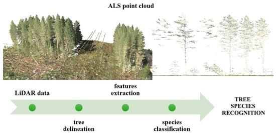
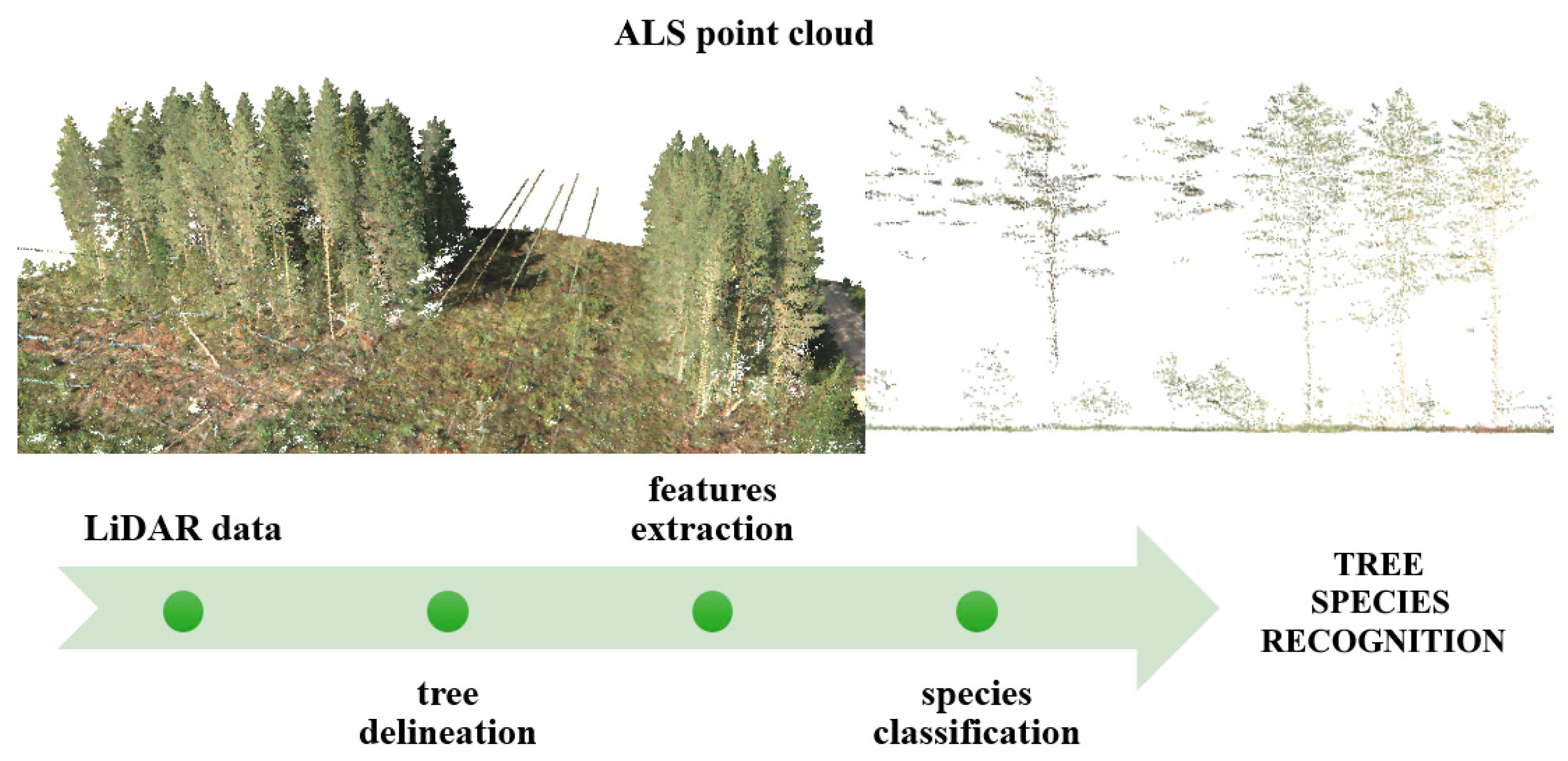
1. Introduction
- What LiDAR features are the most effective for tree species classification?
- What is the most effective classification algorithm to take maximum advantage of the information extracted from LiDAR data to potentially increase the accuracy of tree species classification?
2. Materials and Methods
2.1. Review Approach
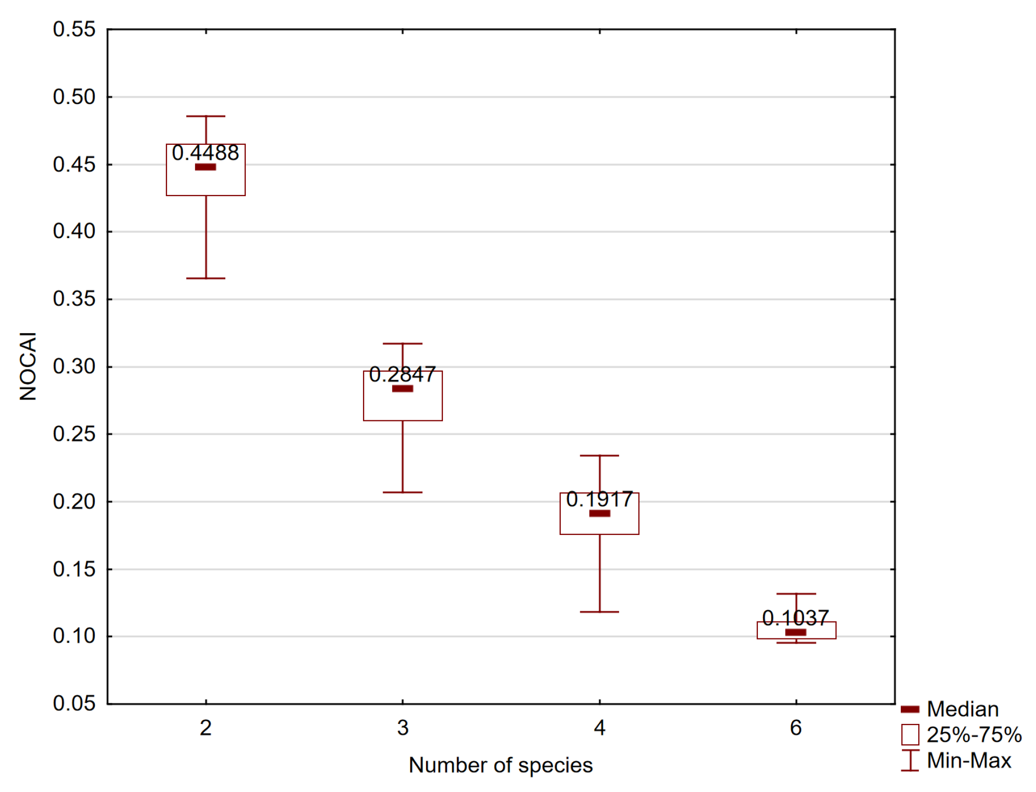
2.2. Accuracy of Species Classification
- N—the total number of samples,
- —the value on the diagonal of the confusion matrix,
- m—the number of classes/species, and
- , —the sums of values on the ith row and ith column, respectively.
- —overall accuracy, and
- k—the number of identified species ( is expected to be achieved if trees were randomly assigned to a species).
2.3. Lidar Features for Tree Species Classification
2.3.1. Geometric—Point Cloud
2.3.2. Radiometric—Intensity and Reflection Type
2.3.3. Full-Waveform Metrics
2.4. Seasonal Tree Condition
2.5. Classification Algorithms
2.5.1. Decision Trees and Random Forest
2.5.2. Support Vector Machine
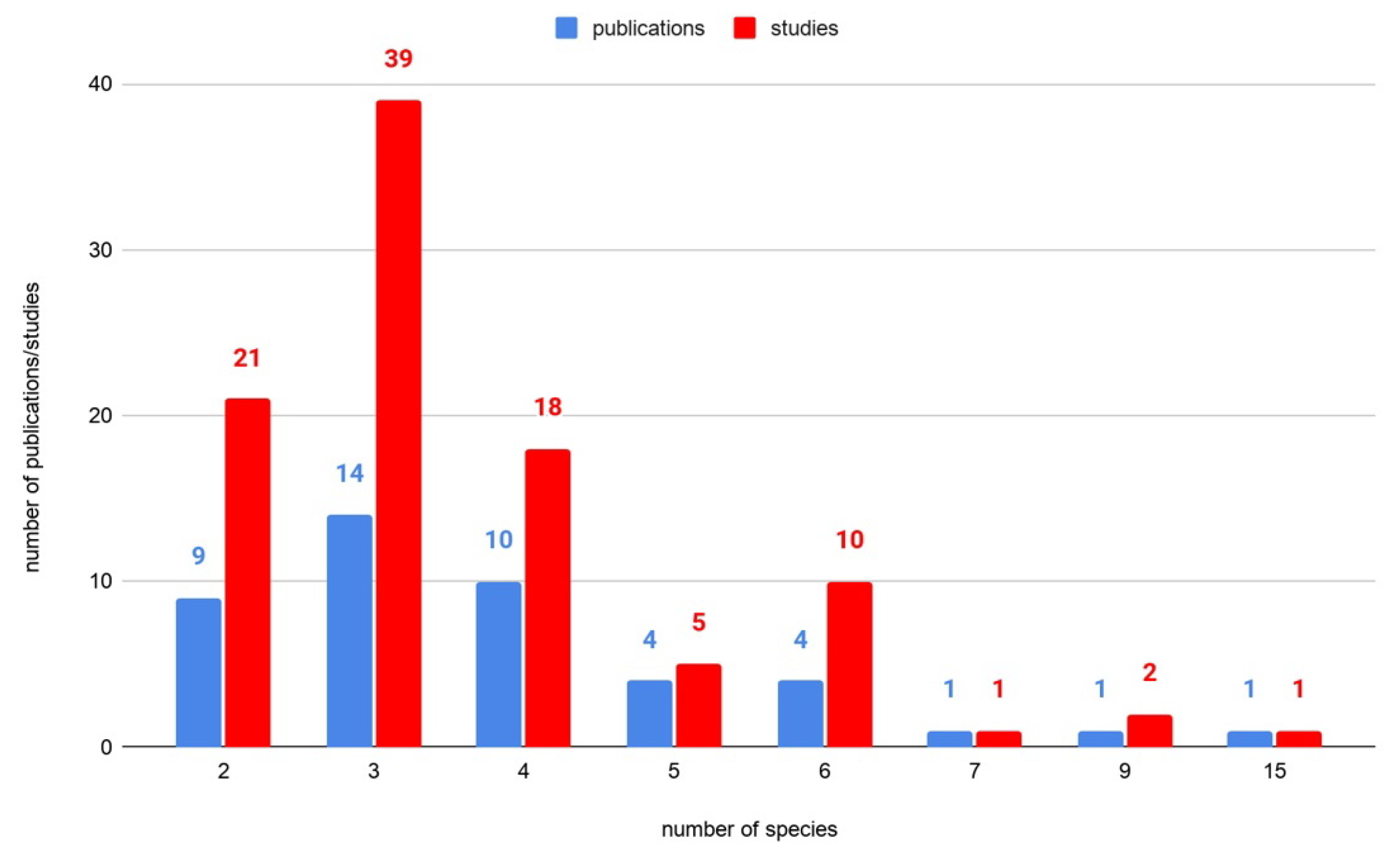
3. Results
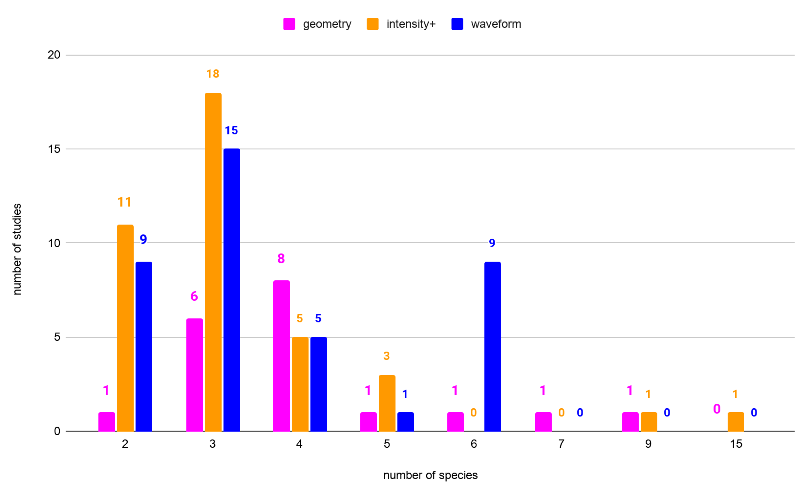
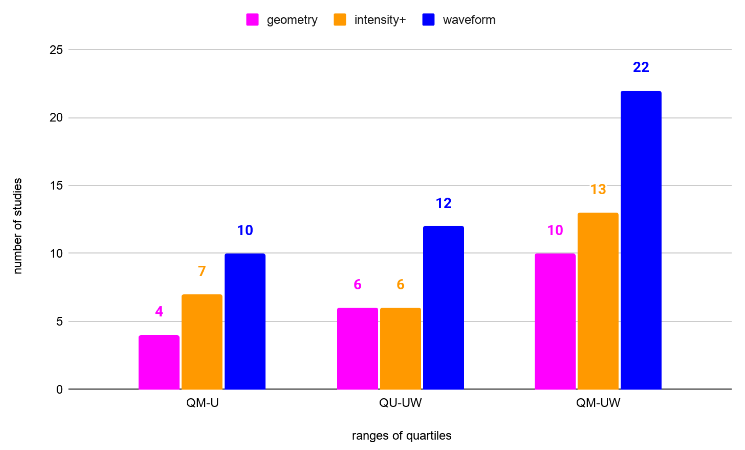
- geometry (G)—geometric features: statistics, point distribution, vertical profile, shape;
- intensity+ (I+)—radiometric features, intensity metrics combined with geometric features, intensity features from three Multispectral Laser Scanning channels;
- waveform (WF)—features extracted from the full-waveform decomposition, full-waveform metrics combined with other metrics.
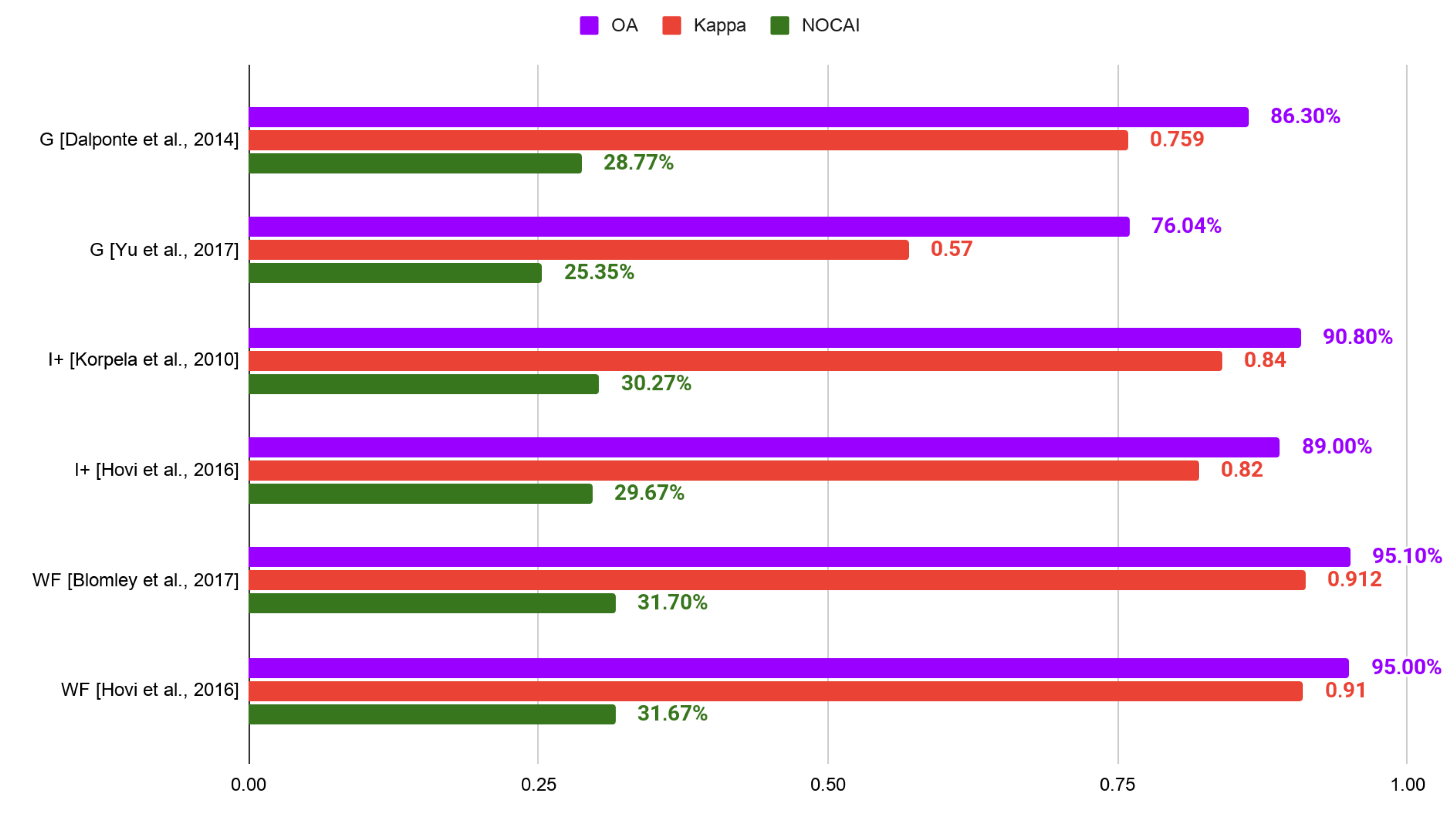
3.1. Effectiveness of the Features Groups in Species Classification
3.2. Effectiveness of the Classifiers in Species Classification
4. Conclusions and Discussion
Author Contributions
Funding
Institutional Review Board Statement
Informed Consent Statement
Data Availability Statement
Conflicts of Interest
Abbreviations
| ABA | Area-Based Approach |
| ALS | Airborne Laser Scanning |
| CHM | Canopy Height Model |
| CNN | Convolutional Neural Network |
| DL | Deep learning |
| G | geometry features group |
| GPS | Global Positioning System |
| I+ | radiometric features group |
| IMU | Inertial Measurement Unit |
| ITC | Individual Tree Crown |
| kNN | k-nearest neighbors |
| LiDAR | Light Detection and Ranging |
| LR | Logistic Regression |
| MLC | Maximum-Likelihood Classifier |
| MLS | Multispectral Laser Scanning |
| NOCAI | Number of Categories Adapted Index |
| OA | Overall Accuracy |
| QM-U | quartile range from the median to upper quartile (75%) |
| QM-UW | quartile range from the median to the upper whisker |
| QU-UW | quartile range from upper quartile (75%) to the upper whisker |
| PA | Producer’s Accuracy |
| RF | Random Forest |
| RS | Remote Sensing |
| SVM | Support Vector Machine |
| TLS | Terrestrial Laser Scanning |
| UAV | Unmanned Aerial Vehicle |
| WF | full-waveform features group |
| WSVM | Weighted Support Vector Machine |
| 2D | two-dimensional |
| 3D | three-dimensional |
Appendix A

| Number of Species | OA | NOCAI | Article | |
|---|---|---|---|---|
| 2 | 95.0% | N/A | 47.50% | [75] |
| 3 | 88.6% | N/A | 29.53% | [87] |
| 3 | 86.3% | 0.759 | 28.77% | [63] |
| 3 | 85.4% (DM) | 0.739 | 28.47% | [63] |
| 3 | 83.15% (DM) | N/A | 27.72% | [61] |
| 3 | 76.04% | 0.57 | 25.35% | [34] |
| 3 | 62.1% | N/A | 20.70% | [81] |
| 4 | 93.7% | N/A | 23.43% | [78] |
| 4 | 89.7% | 0.86 | 22.43% | [66] |
| 4 | 85% | N/A | 21.25% | [79] |
| 4 | 82.5% | N/A | 20.63% | [79] |
| 4 | 77.5% | 0.7 | 19.38% | [77] |
| 4 | 68% | N/A | 17.00% | [35] |
| 4 | 65% | N/A | 16.25% | [79] |
| 4 | 47.27% | N/A | 11.82% | [4] |
| 5 | 87.54% | 0.81 | 17.51% | [83] |
| 6 | 79% | 0.75 | 13.17% | [67] |
| 7 | 50.5% | 0.39 | 7.21% | [66] |
| 9 | 41.3% | N/A | 4.59% | [76] |
| Number of Species | OA | NOCAI | Article | |
|---|---|---|---|---|
| 2 | 97.1% | 0.94 | 48.55% | [40] |
| 2 | 97% | N/A | 48.50% | [113] |
| 2 | 90.6% | N/A | 45.30% | [85] |
| 2 | 90.0% | 0.80 | 45.00% | [40] |
| 2 | 89% | N/A | 44.50% | [113] |
| 2 | 86.9% | 0.74 | 43.42% | [40] |
| 2 | 86% | N/A | 43.00% | [113] |
| 2 | 83.4% | N/A | 41.70% | [85] |
| 2 | 83% | N/A | 41.50% | [113] |
| 2 | 78% | N/A | 39.00% | [113] |
| 2 | 73.1% | N/A | 36.55% | [85] |
| 3 | 92.8% | N/A | 30.93% | [87] |
| 3 | 90.8% (DM) | 0.84 | 30.27% | [43] |
| 3 | 89% | 0.82 | 29.67% | [60] |
| 3 | 88.2% | 0.79 | 29.40% | [27] |
| 3 | 88% | 0.82 | 29.33% | [62] |
| 3 | 88% | 0.79 | 29.33% | [60] |
| 3 | 85.42% | 0.75 | 28.47% | [34] |
| 3 | 85% (DM) | 0.75 | 28.33% | [60] |
| 3 | 85.0% | 0.72 | 28.33% | [27] |
| 3 | 83% | 0.71 | 27.67% | [60] |
| 3 | 82% (DM) | 0.71 | 27.33% | [60] |
| 3 | 81.60% | 0.68 | 27.20% | [34] |
| 3 | 78.1% | N/A | 26.03% | [100] |
| 3 | 78% (DM) | 0.64 | 26.00% | [60] |
| 3 | 78% | 0.64 | 26.00% | [60] |
| 3 | 75.4% | N/A | 25.13% | [87] |
| 3 | 74.38% | 0.56 | 24.79% | [5] |
| 3 | 74% (DM) | 0.57 | 24.67% | [60] |
| 4 | 92.5% | N/A | 23.13% | [79] |
| 4 | 80% | N/A | 20.00% | [79] |
| 4 | 75% | N/A | 18.75% | [35] |
| 4 | 73% | N/A | 18.25% | [35] |
| 4 | 68.0% | 0.56 | 17.60% | [80] |
| 5 | 92.35% | 0.88 | 18.47% | [83] |
| 5 | 69.3% | 0.58 | 13.86% | [68] |
| 5 | 65.1% | 0.57 | 13.02% | [59] |
| 9 | 76.5% | N/A | 8.50% | [76] |
| 15 | 61% | 0.58 | 4.07% | [64] |
| Number of Species | OA | NOCAI | Article | |
|---|---|---|---|---|
| 2 | 95.7% | 0.92 | 47.85% | [84] |
| 2 | 93.45% | 0.61 | 46.73% | [114] |
| 2 | 93.0% | 0.72 | 46.5% | [37] |
| 2 | 92.96% | 0.570 | 46.48% | [114] |
| 2 | 91.7% | N/A | 45.85% | [36] |
| 2 | 89.76% | 0.389 | 44.88% | [114] |
| 2 | 86.2% | 0.72 | 43.10% | [91] |
| 2 | 85.4% | 0.71 | 42.70% | [84] |
| 2 | 84.4% | 0.69 | 42.20% | [91] |
| 3 | 95.1% | 0.912 | 31.70% | [99] |
| 3 | 95% | 0.91 | 31.67% | [60] |
| 3 | 94.8% | 0.905 | 31.60% | [99] |
| 3 | 94.5% | 0.901 | 31.50% | [99] |
| 3 | 92% | 0.86 | 30.67% | [60] |
| 3 | 92% | 0.86 | 30.67% | [60] |
| 3 | 91% (DM) | 0.86 | 30.33% | [60] |
| 3 | 88% (DM) | 0.8 | 29.33% | [60] |
| 3 | 88% | 0.79 | 29.33% | [60] |
| 3 | 87% (DM) | 0.79 | 29.00% | [60] |
| 3 | 84% (DM) | 0.74 | 28.00% | [60] |
| 3 | 85.0% | 0.62 | 28.33% | [94] |
| 3 | 75.0% | N/A | 25.00% | [115] |
| 3 | 73.4% | N/A | 24.47% | [81] |
| 3 | 71.5% | N/A | 23.83% | [81] |
| 4 | 80.4% | N/A | 20.10% | [36] |
| 4 | 79.22% | N/A | 19.81% | [4] |
| 4 | 75.8% | 0.68 | 18.95% | [91] |
| 4 | 73.2% | 0.64 | 18.30% | [91] |
| 4 | 53% | 0.44 | 13.25% | [42] |
| 5 | 85.4% | 0.817 | 17.08% | [103] |
| 6 | 68.6% | 0.62 | 11.43% | [91] |
| 6 | 66.5% | 0.58 | 11.08% | [86] |
| 6 | 66.1% | 0.59 | 11.02% | [91] |
| 6 | 62.4% | 0.54 | 10.40% | [86] |
| 6 | 62.0% | 0.51 | 10.33% | [86] |
| 6 | 60.0% | 0.49 | 10.00% | [86] |
| 6 | 59.0% | N/A | 9.83% | [36] |
| 6 | 58.2% | 0.47 | 9.70% | [86] |
| 6 | 57.1% | 0.46 | 9.52% | [86] |
| Number of Species | Quartile | Feature Group | OA | Article | |
|---|---|---|---|---|---|
| 2 | QU-UW | intensity+ | 97.1% | 0.94 | [40] |
| 2 | QU-UW | intensity+ | 97% | N/A | [113] |
| 2 | QU-UW | waveform | 95.7% | 0.92 | [84] |
| 2 | QU-UW | geometry | 95.0% | N/A | [75] |
| 2 | QU-UW | waveform | 93.45% | 0.61 | [114] |
| 2 | QU-UW | waveform | 93.0% | 0.72 | [37] |
| 2 | QM-U | waveform | 92.96% | 0.570 | [114] |
| 2 | QM-U | waveform | 91.7% | N/A | [36] |
| 2 | QM-U | intensity+ | 90.6% | N/A | [85] |
| 2 | QM-U | intensity+ | 90.0% | 0.80 | [40] |
| 2 | QM-U | waveform | 89.76% | 0.389 | [114] |
| 3 | QU-UW | waveform | 95.1% | 0.912 | [99] |
| 3 | QU-UW | waveform | 95% | 0.91 | [60] |
| 3 | QU-UW | waveform | 94.8% | 0.905 | [99] |
| 3 | QU-UW | waveform | 94.5% | 0.901 | [99] |
| 3 | QU-UW | intensity+ | 92.8% | N/A | [87] |
| 3 | QU-UW | waveform | 92% | 0.86 | [60] |
| 3 | QU-UW | waveform | 92% | 0.86 | [60] |
| 3 | QU-UW | waveform | 91% | 0.86 | [60] |
| 3 | QU-UW | intensity+ | 90.8% | 0.84 | [43] |
| 3 | QU-UW | intensity+ | 89% | 0.82 | [60] |
| 3 | QM-U | geometry | 88.6% | N/A | [87] |
| 3 | QM-U | intensity+ | 88.2% | 0.79 | [27] |
| 3 | QM-U | intensity+ | 88% | 0.82 | [62] |
| 3 | QM-U | waveform | 88% | 0.8 | [60] |
| 3 | QM-U | intensity+ | 88% | 0.79 | [60] |
| 3 | QM-U | waveform | 88% | 0.79 | [60] |
| 3 | QM-U | waveform | 87% | 0.79 | [60] |
| 3 | QM-U | geometry | 86.3% | 0.759 | [63] |
| 3 | QM-U | intensity+ | 85.42% | 0.75 | [34] |
| 3 | QM-U | geometry | 85.4% | 0.739 | [63] |
| 4 | QU-UW | geometry | 93.7% | N/A | [78] |
| 4 | QU-UW | intensity+ | 92.5% | N/A | [79] |
| 4 | QU-UW | geometry | 89.7% | 0.86 | [66] |
| 4 | QU-UW | geometry | 85% | N/A | [79] |
| 4 | QU-UW | geometry | 82.5% | N/A | [79] |
| 4 | QM-U | waveform | 80.4% | N/A | [36] |
| 4 | QM-U | intensity+ | 80% | N/A | [79] |
| 4 | QM-U | waveform | 79.22% | N/A | [4] |
| 4 | QM-U | geometry | 77.5% | 0.7 | [77] |
| 6 | QU-UW | geometry | 79% | 0.75 | [67] |
| 6 | QU-UW | waveform | 68.6% | 0.62 | [91] |
| 6 | QU-UW | waveform | 66.5% | 0.58 | [86] |
| 6 | QM-U | waveform | 66.1% | 0.59 | [91] |
| 6 | QM-U | waveform | 62.4% | 0.54 | [86] |
References
- White, J.C.; Coops, N.C.; Wulder, M.A.; Vastaranta, M.; Hilker, T.; Tompalski, P. Remote sensing technologies for enhancing forest inventories: A review. Can. J. Remote Sens. 2016, 42, 619–641. [Google Scholar] [CrossRef]
- Kangas, A.; Maltamo, M. Forest Inventory: Methodology and Applications; Springer Science & Business Media: Dordrecht, The Netherlands, 2006; Volume 10. [Google Scholar] [CrossRef]
- Dalponte, M.; Bruzzone, L.; Gianelle, D. Tree species classification in the Southern Alps based on the fusion of very high geometrical resolution multispectral/hyperspectral images and LiDAR data. Remote Sens. Environ. 2012, 123, 258–270. [Google Scholar] [CrossRef]
- Heinzel, J.; Koch, B. Investigating multiple data sources for tree species classification in temperate forest and use for single tree delineation. Int. J. Appl. Earth Obs. Geoinf. 2012, 18, 101–110. [Google Scholar] [CrossRef]
- Ørka, H.; Dalponte, M.; Gobakken, T.; Næsset, E.; Ene, L. Characterizing forest species composition using multiple remote sensing data sources and inventory approaches. Scand. J. For. Res. 2013, 28. [Google Scholar] [CrossRef]
- Peterson, D.L.; Aber, J.D.; Matson, P.A.; Card, D.H.; Swanberg, N.; Wessman, C.; Spanner, M. Remote sensing of forest canopy and leaf biochemical contents. Remote Sens. Environ. 1988, 24, 85–108. [Google Scholar] [CrossRef]
- Baret, F.; Vanderbilt, V.C.; Steven, M.D.; Jacquemoud, S. Use of spectral analogy to evaluate canopy reflectance sensitivity to leaf optical properties. Remote Sens. Environ. 1994, 48, 253–260. [Google Scholar] [CrossRef]
- Asner, G.P.; Martin, R.E. Airborne spectranomics: Mapping canopy chemical and taxonomic diversity in tropical forests. Front. Ecol. Environ. 2009, 7, 269–276. [Google Scholar] [CrossRef]
- Schimel, D.S.; Asner, G.P.; Moorcroft, P. Observing changing ecological diversity in the Anthropocene. Front. Ecol. Environ. 2013, 11, 129–137. [Google Scholar] [CrossRef]
- Baldeck, C.A.; Asner, G.P.; Martin, R.E.; Anderson, C.B.; Knapp, D.E.; Kellner, J.R.; Wright, S.J. Operational tree species mapping in a diverse tropical forest with airborne imaging spectroscopy. PLoS ONE 2015, 10, e0118403. [Google Scholar] [CrossRef]
- Brosofske, K.D.; Froese, R.E.; Falkowski, M.J.; Banskota, A. A review of methods for mapping and prediction of inventory attributes for operational forest management. For. Sci. 2014, 60, 733–756. [Google Scholar] [CrossRef]
- Maltamo, M.; Næsset, E.; Vauhkonen, J. Forestry applications of airborne laser scanning. Concepts Case Stud. Manag. Ecosys 2014, 27, 460. [Google Scholar] [CrossRef]
- Kelly, M.; Di Tommaso, S. Mapping forests with Lidar provides flexible, accurate data with many uses. Calif. Agric. 2015, 69, 14–20. [Google Scholar] [CrossRef]
- Krzystek, P.; Serebryanyk, A.; Schnörr, C.; Červenka, J.; Heurich, M. Large-Scale Mapping of Tree Species and Dead Trees in Šumava National Park and Bavarian Forest National Park Using Lidar and Multispectral Imagery. Remote Sens. 2020, 12, 661. [Google Scholar] [CrossRef]
- Bachman, C.G. Laser Radar Systems and Techniques; Artech House: Dedham, MA, USA, 1979. [Google Scholar]
- Wehr, A.; Lohr, U. Airborne laser scanning—An introduction and overview. ISPRS J. Photogramm. Remote Sens. 1999, 54, 68–82. [Google Scholar] [CrossRef]
- Pritchard, D.; Sperner, J.; Hoepner, S.; Tenschert, R. Terrestrial laser scanning for heritage conservation: The Cologne Cathedral documentation project. ISPRS Ann. Photogramm. Remote Sens. Spat. Inf. Sci. 2017, 4. [Google Scholar] [CrossRef]
- Pérez-Álvarez, R.; de Luis, J.; Pereda-García, R.; Fernández-Maroto, G.; Malagón-Picón, B. 3D Documentation with TLS of Caliphal Gate (Ceuta, Spain). Appl. Sci. 2020, 10, 5377. [Google Scholar] [CrossRef]
- Pu, S. Generating building outlines from terrestrial laser scanning. ISPRS08 B 2008, 5, 451–455. [Google Scholar]
- Nowak, R.; Orłowicz, R.; Rutkowski, R. Use of TLS (LiDAR) for building diagnostics with the example of a historic building in Karlino. Buildings 2020, 10, 24. [Google Scholar] [CrossRef]
- Suchocki, C.; Damięcka-Suchocka, M.; Katzer, J.; Janicka, J.; Rapinski, J.; Stałowska, P. Remote Detection of Moisture and Bio-Deterioration of Building Walls by Time-Of-Flight and Phase-Shift Terrestrial Laser Scanners. Remote Sens. 2020, 12, 1708. [Google Scholar] [CrossRef]
- Guan, H.; Li, J.; Cao, S.; Yu, Y. Use of mobile LiDAR in road information inventory: A review. Int. J. Image Data Fusion 2016, 7, 219–242. [Google Scholar] [CrossRef]
- Truong-Hong, L.; Laefer, D.F. Documentation of bridges by terrestrial laser scanner. In Proceedings of the IABSE Geneva Conference 2015, Geneva, Switzerland, 23–25 September 2015. [Google Scholar] [CrossRef]
- Artese, S.; Zinno, R. TLS for Dynamic Measurement of the Elastic Line of Bridges. Appl. Sci. 2020, 10, 1182. [Google Scholar] [CrossRef]
- Hyyppä, J.; Yu, X.; Hyyppä, H.; Vastaranta, M.; Holopainen, M.; Kukko, A.; Kaartinen, H.; Jaakkola, A.; Vaaja, M.; Koskinen, J.; et al. Advances in forest inventory using airborne laser scanning. Remote Sens. 2012, 4, 1190–1207. [Google Scholar] [CrossRef]
- Latifi, H.; Fassnacht, F.E.; Müller, J.; Tharani, A.; Dech, S.; Heurich, M. Forest inventories by LiDAR data: A comparison of single tree segmentation and metric-based methods for inventories of a heterogeneous temperate forest. Int. J. Appl. Earth Obs. Geoinf. 2015, 42, 162–174. [Google Scholar] [CrossRef]
- Kukkonen, M.; Maltamo, M.; Korhonen, L.; Packalen, P. Multispectral airborne LiDAR data in the prediction of boreal tree species composition. IEEE Trans. Geosci. Remote Sens. 2019, 57, 3462–3471. [Google Scholar] [CrossRef]
- Prieto, I.; Izkara, J.L.; Usobiaga, E. The application of lidar data for the solar potential analysis based on urban 3D model. Remote Sens. 2019, 11, 2348. [Google Scholar] [CrossRef]
- Wang, X.; Chan, T.O.; Liu, K.; Pan, J.; Luo, M.; Li, W.; Wei, C. A robust segmentation framework for closely packed buildings from airborne LiDAR point clouds. Int. J. Remote Sens. 2020, 41, 5147–5165. [Google Scholar] [CrossRef]
- Heritage, G.; Large, A. Laser Scanning for the Environmental Sciences; John Wiley & Sons: Hoboken, NJ, USA, 2009. [Google Scholar] [CrossRef]
- Pyysalo, U.; Hyyppa, H. Reconstructing tree crowns from laser scanner data for feature extraction. Int. Arch. Photogramm. Remote Sens. Spat. Inf. Sci. 2002, 34, 218–221. [Google Scholar]
- Solberg, S.; Naesset, E.; Bollandsas, O.M. Single tree segmentation using airborne laser scanner data in a structurally heterogeneous spruce forest. Photogramm. Eng. Remote Sens. 2006, 72, 1369–1378. [Google Scholar] [CrossRef]
- Chamberlain, C.P.; Meador, A.J.S.; Thode, A.E. Airborne lidar provides reliable estimates of canopy base height and canopy bulk density in southwestern ponderosa pine forests. For. Ecol. Manag. 2020, 481, 118695. [Google Scholar] [CrossRef]
- Yu, X.; Hyyppä, J.; Litkey, P.; Kaartinen, H.; Vastaranta, M.; Holopainen, M. Single-sensor solution to tree species classification using multispectral airborne laser scanning. Remote Sens. 2017, 9, 108. [Google Scholar] [CrossRef]
- Krüger geb. Amiri, N.; Heurich, M.; Krzystek, P.; Skidmore, A. Feature Relevance Assessment of Multispectral Airborne LiDAR Data for Tree Species Classification. ISPRS Int. Arch. Photogramm. Remote Sens. Spat. Inf. Sci. 2018, XLII-3, 31–34. [Google Scholar] [CrossRef]
- Heinzel, J.; Koch, B. Exploring full-waveform LiDAR parameters for tree species classification. Int. J. Appl. Earth Obs. Geoinf. 2011, 13, 152–160. [Google Scholar] [CrossRef]
- Yao, W.; Krzystek, P.; Heurich, M. Tree species classification and estimation of stem volume and DBH based on single tree extraction by exploiting airborne full-waveform LiDAR data. Remote Sens. Environ. 2012, 123, 368–380. [Google Scholar] [CrossRef]
- Naesset, E. Estimating timber volume of forest stands using airborne laser scanner data. Remote Sens. Environ. 1997, 61, 246–253. [Google Scholar] [CrossRef]
- Hyyppa, J.; Kelle, O.; Lehikoinen, M.; Inkinen, M. A segmentation-based method to retrieve stem volume estimates from 3-D tree height models produced by laser scanners. IEEE Trans. Geosci. Remote Sens. 2001, 39, 969–975. [Google Scholar] [CrossRef]
- Ørka, H.O.; Næsset, E.; Bollandsås, O.M. Effects of different sensors and leaf-on and leaf-off canopy conditions on echo distributions and individual tree properties derived from airborne laser scanning. Remote Sens. Environ. 2010, 114, 1445–1461. [Google Scholar] [CrossRef]
- Bont, L.; Hill, A.; Waser, L.; Bürgi, A.; Ginzler, C.; Blattert, C. Airborne-laser-scanning-derived auxiliary information discriminating between broadleaf and conifer trees improves the accuracy of models for predicting timber volume in mixed and heterogeneously structured forests. For. Ecol. Manag. 2020, 459, 117856. [Google Scholar] [CrossRef]
- Sarrazin, D.; van Aardt, J.; Asner, G.; Mcglinchy, J.; Messinger, D.; Wu, J. Fusing small-footprint waveform LiDAR and hyperspectral data for canopy-level species classification and herbaceous biomass modeling in savanna ecosystems. Can. J. Remote Sens. 2011, 37, 653–665. [Google Scholar] [CrossRef]
- Korpela, I.; Ørka, H.; Maltamo, M.; Tokola, T.; Hyyppä, J.; Tokola, M.; Maltamo, T. Tree Species Classification Using Airborne LiDAR—Effects of Stand and Tree Parameters, Downsizing of Training Set, Intensity Normalization, and Sensor Type. Silva Fenn. 2010, 44. [Google Scholar] [CrossRef]
- Culvenor, D. A Spatial Clustering Approach to Automated Tree Crown Delineation; Pacific Forestry Centre: Victoria, BC, Canada, 1998; pp. 67–88. [Google Scholar]
- Voss, M.; Sugumaran, R. Seasonal effect on tree species classification in an urban environment using hyperspectral data, LiDAR, and an object-oriented approach. Sensors 2008, 8, 3020–3036. [Google Scholar] [CrossRef]
- Reitberger, J.; Schnörr, C.; Krzystek, P.; Stilla, U. 3D segmentation of single trees exploiting full waveform LIDAR data. ISPRS J. Photogramm. Remote Sens. 2009, 64, 561–574. [Google Scholar] [CrossRef]
- Yu, X.; Hyyppä, J.; Holopainen, M.; Vastaranta, M. Comparison of Area-Based and Individual Tree-Based Methods for Predicting Plot-Level Forest Attributes. Remote Sens. 2010, 2, 1481–1495. [Google Scholar] [CrossRef]
- Yao, W. A Sensitivity Analysis for a Novel Individual Tree Segmentation Algorithm Using 3D Lidar Point Cloud Data; Silvilaser: Vancouver, BC, Canada, 2012. [Google Scholar]
- Eysn, L.; Hollaus, M.; Lindberg, E.; Berger, F.; Monnet, J.M.; Dalponte, M.; Kobal, M.; Pellegrini, M.; Lingua, E.; Mongus, D.; et al. A Benchmark of Lidar-Based Single Tree Detection Methods Using Heterogeneous Forest Data from the Alpine Space. Forests 2015, 6, 1721–1747. [Google Scholar] [CrossRef]
- Smith, S.; Holland, D.; Longley, P. The importance of understanding error in lidar digital elevation models. Int. Arch. Photogramm. Remote Sens. Spat. Inf. Sci. 2004, 35, 996–1001. [Google Scholar]
- Tiede, D.; Hochleitner, G.; Blaschke, T. A full GIS-based workflow for tree identification and tree crown delineation using laser scanning. ISPRS Workshop CMRT 2005, 5, 2005. [Google Scholar]
- Zhao, K.; Popescu, S. Hierarchical watershed segmentation of canopy height model for multi-scale forest inventory. Proc. ISPRS Work. Group 2007, 442, 436. [Google Scholar]
- Zhong, L.; Cheng, L.; Xu, H.; Wu, Y.; Chen, Y.; Li, M. Segmentation of Individual Trees From TLS and MLS Data. IEEE J. Sel. Top. Appl. Earth Obs. Remote Sens. 2016, 1–14. [Google Scholar] [CrossRef]
- Xu, S.; Ye, N.; Xu, S.; Zhu, F. A supervoxel approach to the segmentation of individual trees from LiDAR point clouds. Remote Sens. Lett. 2018, 9, 515–523. [Google Scholar] [CrossRef]
- Xu, Y.; Sun, Z.; Hoegner, L.; Stilla, U.; Yao, W. Instance Segmentation of Trees in Urban Areas from MLS Point Clouds Using Supervoxel Contexts and Graph-Based Optimization. In Proceedings of the 10th IAPR Workshop on Pattern Recognition in Remote Sensing (PRRS), Beijing, China, 19–20 August 2018; pp. 1–5. [Google Scholar] [CrossRef]
- Anandakumar, R.; Nidamanuri, R.; Krishnan, R. Assessment of various parameters on 3D semantic object-based point cloud labelling on urban LiDAR dataset. Geocarto Int. 2018, 34, 1–29. [Google Scholar] [CrossRef]
- Anandakumar, R.; Nidamanuri, R.; Krishnan, R. Individual tree detection from airborne laser scanning data based on supervoxels and local convexity. Remote Sens. Appl. Soc. Environ. 2019, 15, 100242. [Google Scholar] [CrossRef]
- Ørka, H.; Næsset, E.; Bollandsås, O. Classifying species of individual trees by intensity and structure features derived from airborne laser scanner data. Remote Sens. Environ. 2009, 113, 1163–1174. [Google Scholar] [CrossRef]
- Shi, Y.; Skidmore, A.; Holzwarth, S.; Heiden, U.; Pinnel, N.; Zhu, X.; Heurich, M. Tree species classification using plant functional traits from LiDAR and hyperspectral data. Int. J. Appl. Earth Obs. Geoinf. 2018, 73. [Google Scholar] [CrossRef]
- Hovi, A.; Korhonen, L.; Vauhkonen, J.; Korpela, I. LiDAR waveform features for tree species classification and their sensitivity to tree- and acquisition related parameters. Remote Sens. Environ. 2016, 173, 224–237. [Google Scholar] [CrossRef]
- Ba, A.; Laslier, M.; Dufour, S.; Hubert-Moy, L. Riparian Trees Genera Identification Based on Leaf-on/Leaf-off Airborne Laser Acanner Data and Machine Learning Classifiers in Northern France. Int. J. Remote Sens. 2019. [Google Scholar] [CrossRef]
- Holmgren, J.; Persson, A.; Söderman, U. Species identification of individual trees by combining high resolution LiDAR data with multi-spectral images. Int. J. Remote Sens. Int. Remote Sens. 2008, 29, 1537–1552. [Google Scholar] [CrossRef]
- Dalponte, M.; Ørka, H.; Ene, L.; Gobakken, T.; Næsset, E. Tree crown delineation and tree species classification in boreal forests using hyperspectral and ALS data. Remote Sens. Environ. 2014, 140, 306–317. [Google Scholar] [CrossRef]
- Liu, L.; Coops, N.; Aven, N.; Pang, Y. Mapping urban tree species using integrated airborne hyperspectral and LiDAR remote sensing data. Remote Sens. Environ. 2017, 200, 170–182. [Google Scholar] [CrossRef]
- Liao, W.; Van Coillie, F.; Gao, L.; Li, L.; Chanussot, J. Deep Learning for Fusion of APEX Hyperspectral and Full-waveform LiDAR Remote Sensing Data for Tree Species Mapping. IEEE Access 2018, 6, 68716–68729. [Google Scholar] [CrossRef]
- Yang, G.; Zhao, Y.; Li, B.; Ma, Y.; Li, R.; Jing, J.; Dian, Y. Tree Species Classification by Employing Multiple Features Acquired from Integrated Sensors. J. Sens. 2019, 2019, 1–12. [Google Scholar] [CrossRef]
- Li, Q.; Wong, F.; Fung, T. Classification of Mangrove Species Using Combined WordView-3 and LiDAR Data in Mai Po Nature Reserve, Hong Kong. Remote Sens. 2019, 11, 2114. [Google Scholar] [CrossRef]
- Shi, Y.; Skidmore, A.; Heurich, M. Improving LiDAR-based tree species mapping in Central European mixed forests using multi-temporal digital aerial colour-infrared photographs. Int. J. Appl. Earth Obs. Geoinf. 2019, 84. [Google Scholar] [CrossRef]
- Cohen, J. A Coefficient of Agreement for Nominal Scales. Psychol. Bull. 1960, 20, 37. [Google Scholar] [CrossRef]
- Landis, J.; Koch, G. The Measurement of Observer Agreement For Categorical Data. Biometrics 1977, 33, 159–174. [Google Scholar] [CrossRef] [PubMed]
- Wang, K.; Liu, X. A Review: Individual Tree Species Classification Using Integrated Airborne LiDAR and Optical Imagery with a Focus on the Urban Environment. Forests 2018, 10, 1. [Google Scholar] [CrossRef]
- Zhang, C.; Qiu, F. Mapping individual tree species in an urban forest using airborne lidar data and hyperspectral imagery. Photogramm. Eng. Remote Sens. 2012, 78, 1079–1087. [Google Scholar] [CrossRef]
- Koenig, K.; Höfle, B. Full-Waveform Airborne Laser Scanning in Vegetation Studies—A Review of Point Cloud and Waveform Features for Tree Species Classification. Forests 2016, 7, 198. [Google Scholar] [CrossRef]
- Ørka, H.; Næsset, E.; Bollandsås, O. Utilizing Airborne Laser Intensity for Tree Species Classification. Int. Arch. Photogramm. Remote Sens. Spat. Inf. Sci. 2012, 36, 300–304. [Google Scholar]
- Holmgren, J.; Persson, A. Identifying species of individual trees using airborne laser scanner. Remote Sens. Environ. 2004, 90, 415–423. [Google Scholar] [CrossRef]
- Axelsson, A.; Lindberg, E.; Olsson, H. Exploring Multispectral ALS Data for Tree Species Classification. Remote Sens. 2018, 10, 183. [Google Scholar] [CrossRef]
- Li, J.; Hu, B.; Noland, T. Classification of tree species based on structural features derived from high density LiDAR data. Agric. For. Meteorol. 2013, 171–172, 104–114. [Google Scholar] [CrossRef]
- Harikumar, A.; Bovolo, F.; Bruzzone, L. An Internal Crown Geometric Model for Conifer Species Classification With High-Density LiDAR Data. IEEE Trans. Geosci. Remote Sens. 2017, 55, 2924–2940. [Google Scholar] [CrossRef]
- Lin, Y.; Hyyppä, J. A comprehensive but efficient framework of proposing and validating feature parameters from airborne LiDAR data for tree species classification. Int. J. Appl. Earth Obs. Geoinf. 2016, 46, 45–55. [Google Scholar] [CrossRef]
- Suratno, A.; Seielstad, C.; Queen, L. Tree species identification in mixed coniferous forest using airborne laser scanning. ISPRS J. Photogramm. Remote Sens. ISPRS Photogramm. 2009, 64, 683–693. [Google Scholar] [CrossRef]
- Yu, X.; Litkey, P.; Hyyppä, J.; Holopainen, M.; Vastaranta, M. Assessment of Low Density Full-Waveform Airborne Laser Scanning for Individual Tree Detection and Tree Species Classification. Forests 2014, 5, 1011–1031. [Google Scholar] [CrossRef]
- Höfle, B.; Hollaus, M.; Hagenauer, J. Urban vegetation detection using radiometrically calibrated small-footprint full-waveform airborne LiDAR data. ISPRS J. Photogramm. Remote Sens. 2012, 67, 134–147. [Google Scholar] [CrossRef]
- You, H.; Lei, P.; Li, M.; Ruan, F. Forest Species Classification Based on Three-dimensional Coordinate and Intensity Information of Airborne LiDAR Data with Random Forest Method. ISPRS Int. Arch. Photogramm. Remote Sens. Spat. Inf. Sci. 2020, XLII-3/W10, 117–123. [Google Scholar] [CrossRef]
- Reitberger, J.; Krzystek, P.; Stilla, U. Analysis of full waveform LIDAR data for the classification of deciduous and coniferous trees. Int. J. Remote Sens. 2008, 29, 1407–1431. [Google Scholar] [CrossRef]
- Kim, S.; Mcgaughey, R.; Andersen, H.E.; Schreuder, G. Tree species differentiation using intensity data derived from leaf-on and leaf-off airborne laser scanner data. Remote Sens. Environ. 2009, 113, 1575–1586. [Google Scholar] [CrossRef]
- Shi, Y.; Skidmore, A.; Heurich, M. Important LiDAR metrics for discriminating forest tree species in Central Europe. ISPRS J. Photogramm. Remote Sens. 2018, 137, 163–174. [Google Scholar] [CrossRef]
- Zhang, Z.; Liu, X. Support vector machines for tree species identification using LiDAR-derived structure and intensity variables. Geocarto Int. 2012, 28, 1–15. [Google Scholar] [CrossRef]
- Budei, B.; St-Onge, B.; Hopkinson, C.; Audet, F.A. Identifying the genus or species of individual trees using a three-wavelength airborne lidar system. Remote Sens. Environ. 2017, 204. [Google Scholar] [CrossRef]
- Pirotti, F. Analysis of full-waveform LiDAR data for forestry applications: A review of investigations and methods. Iforest Biogeosci. For. 2011, 100–106. [Google Scholar] [CrossRef]
- Wagner, W.; Ullrich, A.; Ducic, V.; Melzer, T.; Studnicka, N. Gaussian decomposition and calibration of a novel small-footprint full-waveform digitising airborne laser scanner. ISPRS J. Photogramm. Remote Sens. 2006, 60, 100–112. [Google Scholar] [CrossRef]
- Cao, L.; Coops, N.; Innes, J.; Dai, J.; Ruan, H.; She, G. Tree species classification in subtropical forests using small-footprint full-waveform LiDAR data. Int. J. Appl. Earth Obs. Geoinf. 2016, 49, 39–51. [Google Scholar] [CrossRef]
- Drake, J.B.; Dubayah, R.O.; Clark, D.B.; Knox, R.G.; Blair, J.; Hofton, M.A.; Chazdon, R.L.; Weishampel, J.F.; Prince, S. Estimation of tropical forest structural characteristics using large-footprint LiDAR. Remote Sens. Environ. 2002, 79, 305–319. [Google Scholar] [CrossRef]
- Duong, V. Processing and Application of ICESat Large Footprint Full Waveform Laser Range Data. Ph.D. Thesis, Delft University of Technology, Delft, The Netherlands, 2010. [Google Scholar]
- Hollaus, M.; Mücke, W.; Höfle, B.; Dorigo, W.; Pfeifer, N.; Wagner, W.; Bauerhansl, C.; Regner, B. Tree species classification based on full-waveform airborne laser scanning data. SilviLaser 2009, 54, 14–16. [Google Scholar]
- Zhou, T.; Popescu, S.; Lawing, A.M.; Eriksson, M.; Strimbu, B.; Burkner, P. Bayesian and Classical Machine Learning Methods: A Comparison for Tree Species Classification with LiDAR Waveform Signatures. Remote Sens. 2018, 10, 39. [Google Scholar] [CrossRef]
- Brandtberg, T.; Warner, T.; Landenberger, R.; Mcgraw, J. Detection and analysis of individual leaf-off tree crowns in small footprint, high sampling density lidar data from the eastern deciduous forest in North America. Remote Sens. Environ. 2003, 85, 290–303. [Google Scholar] [CrossRef]
- Wasser, L.; Day, R.; Chasmer, L.; Taylor, A. Influence of Vegetation Structure on Lidar-derived Canopy Height and Fractional Cover in Forested Riparian Buffers During Leaf-Off and Leaf-On Conditions. PLoS ONE 2013, 8, e54776. [Google Scholar] [CrossRef]
- Sumnall, M.; Hill, R.; Hinsley, S. Comparison of small-footprint discrete return and full waveform airborne lidar data for estimating multiple forest variables. Remote Sens. Environ. 2015, 173. [Google Scholar] [CrossRef]
- Blomley, R.; Hovi, A.; Weinmann, M.; Hinz, S.; Korpela, I.; Jutzi, B. Tree species classification using within crown localization of waveform LiDAR attributes. ISPRS J. Photogramm. Remote Sens. 2017, 133, 142–156. [Google Scholar] [CrossRef]
- Vauhkonen, J.; Korpela, I.; Maltamo, M.; Tokola, T. Imputation of single-tree attributes using airborne laser scanning-based height, intensity, and alpha shape metrics. Remote Sens. Environ. 2010, 114, 1263–1276. [Google Scholar] [CrossRef]
- Ballanti, L.; Blesius, L.; Hines, E.; Kruse, B. Tree Species Classification Using Hyperspectral Imagery: A Comparison of Two Classifiers. Remote Sens. 2016, 8, 445. [Google Scholar] [CrossRef]
- Jones, T.; Coops, N.; Sharma, T. Assessing the utility of airborne hyperspectral and LiDAR data for species distribution mapping in the coastal Pacific Northwest, Canada. Remote Sens. Environ. 2010, 114, 2841–2852. [Google Scholar] [CrossRef]
- Vaughn, N.; Moskal, L.; Turnblom, E. Tree Species Detection Accuracies Using Discrete Point Lidar and Airborne Waveform Lidar. Remote Sens. 2012, 4, 377–403. [Google Scholar] [CrossRef]
- Nguyen, H.; Demir, B.; Dalponte, M. Weighted Support Vector Machines for Tree Species Classification Using Lidar Data. In Proceedings of the IGARSS 2019-2019 IEEE International Geoscience and Remote Sensing Symposium, Yokohama, Japan, 28 July–2 August 2019; pp. 6740–6743. [Google Scholar] [CrossRef]
- Breiman, L. Random Forests. Mach. Learn. Vol. 2001, 45, 5–32. [Google Scholar] [CrossRef]
- Cortes, C.; Vapnik, V. Support-vector networks. Chem. Biol. Drug Des. 2009, 297, 273–297. [Google Scholar] [CrossRef]
- Fassnacht, F.; Latifi, H.; Stereńczak, K.; Modzelewska, A.; Lefsky, M.; Waser, L.; Straub, C.; Ghosh, A. Review of studies on tree species classification from remotely sensed data. Remote Sens. Environ. 2016, 186, 64–87. [Google Scholar] [CrossRef]
- Polewski, P.P. Reconstruction of Standing and Fallen Single Dead Trees in Forested Areas from LiDAR Data and Aerial Imagery. Ph.D. Thesis, Technische Universität München, München, Germany, 2017. [Google Scholar]
- Polewski, P.; Yao, W.; Heurich, M.; Krzystek, P.; Stilla, U. Free Shape Context descriptors optimized with genetic algorithm for the detection of dead tree trunks in ALS point clouds. ISPRS Geospat. Week 2015, W5, 41–48. [Google Scholar] [CrossRef]
- Jayathunga, S.; Owari, T.; Tsuyuki, S. Analysis of forest structural complexity using airborne LiDAR data and aerial photography in a mixed conifer–broadleaf forest in northern Japan. J. For. Res. 2018, 29, 479–493. [Google Scholar] [CrossRef]
- Latifi, H.; Heurich, M.; Hartig, F.; Müller, J.; Krzystek, P.; Jehl, H.; Dech, S. Estimating over-and understorey canopy density of temperate mixed stands by airborne LiDAR data. For. Int. J. For. Res. 2016, 89, 69–81. [Google Scholar] [CrossRef]
- Zielewska-Büttner, K.; Heurich, M.; Müller, J.; Braunisch, V. Remotely sensed single tree data enable the determination of habitat thresholds for the three-toed woodpecker (Picoides tridactylus). Remote Sens. 2018, 10, 1972. [Google Scholar] [CrossRef]
- Vauhkonen, J.; Hakala, T.; Suomalainen, J.; Kaasalainen, S.; Nevalainen, O.; Vastaranta, M.; Holopainen, M.; Hyyppä, J. Classification of Spruce and Pine Trees Using Active Hyperspectral LiDAR. IEEE Geosci. Remote Sens. Lett. 2013, 10, 1138–1141. [Google Scholar] [CrossRef]
- Bruggisser, M.; Roncat, A.; Schaepman, M.; Morsdorf, F. Retrieval of higher order statistical moments from full-waveform LiDAR data for tree species classification. Remote Sens. Environ. 2017, 196, 28–41. [Google Scholar] [CrossRef]
- Vaughn, N.; Moskal, L.; Turnblom, E. Fourier transformation of waveform Lidar for species recognition. Remote Sens. Lett. 2011, 2, 347–356. [Google Scholar] [CrossRef]


| Feature | Definition |
|---|---|
| H | Maximum of the normalized height of all points |
| H | Arithmetic mean of normalized height of all points above stated in meters threshold |
| H | Standard deviation of normalized height of all points above stated in meters threshold |
| H | Median of the normalized height of all points |
| H | Range of normalized height of all points above stated in meters threshold |
| HP to HP | 10% to 90% percentiles of normalized height of all points above stated in meters threshold with a 10% increment |
| P | Penetration as a ratio between number of returns below stated meter and total returns |
| CA | Crown area as the area of 2D convex hull |
| CV | Crown volume as the 3D convex hull |
| CD | Crown equivalent diameter calculated from crown area considering crown as a circle |
| As | Asymmetry as a difference between two crown diameters taken in two directions |
| dns | Canopy density |
| D to D | Density at a fixed height. , where i = 1 to 10, is the number of points within ith layer when tree height was divided into 10 intervals starting from specified meter, is the number of all points |
| Feature | Definition |
|---|---|
| I | Minimum of intensity |
| I | Maximum of intensity |
| I | Mean of intensity |
| I | Standard deviation of intensity |
| I | Coefficient of variation of intensity |
| I | Median of intensity |
| I | Skewness of intensity |
| I | Range of intensity |
| I | Kurtosis of intensity |
| I | Intensity value at percentiles from 10% to 90% with 10% increment |
| Feature | Definition |
|---|---|
| I | Minimum of intensity of ith channel |
| I | Maximum of intensity of ith channel |
| I | Mean of intensity of ith channel |
| I | Standard deviation of intensity of ith channel |
| I | Coefficient of variation of intensity of ith channel |
| I | Median of intensity of ith channel |
| I | Skewness of intensity of ith channel |
| I | Range of intensity of ith channel |
| I | Kurtosis of intensity of ith channel |
| I | Percentiles of intensity of ith channel from 10% to 90% with 10% increment |
| I, I, I, I | Intensity computed from combined set of echoes from different channels |
| I/(I + I + I) | Ratios of intensity features, F refers to different single-channel intensity features |
| I/I, I/I, I/I | Ratios of intensity features |
| (I − I)/(I + I) | Index of intensity features |
| Feature | Definition |
|---|---|
| WD | Waveform distance–distance between waveform begin and the ground (last peak) |
| WE | Waveform extent–distance between waveform begin and end |
| HOME | Height of median energy–distance from waveform centroid to the ground (last peak) |
| HTRT | Height of median energy/canopy height ratio |
| FS | Front slope angle–vertical angle from waveform begin to the first peak of canopy return energy |
| NP | Number of peaks–number of detected peaks within each normalized composite waveform |
| H | x% quartile height from 25% to 100% with 25% increment–elevation at x% of the returned energy subtracted by the ground elevation |
| ROUGH | Roughness of outer canopy–distance from the waveform beginning to the first peak |
| RWE | Return waveform energy–the area below the waveform between beginning and end |
| GE | Ground energy–total intensity of the last mode |
| CE | Canopy energy–difference between return waveform energy and ground return energy |
| GRND | Ground return ratio–ground return energy divided by canopy return energy |
| Article | kNN | LDA | LR | MLC | RF | SVM | DL |
|---|---|---|---|---|---|---|---|
| [61] | 83.1% N/A | 82.0% N/A | |||||
| [43] | 73.4% 0.639 | 77.1% 0.628 | 81.7% 0.690 | ||||
| 76.0% 0.681 | 78.9% 0.656 | 83.5% 0.720 | |||||
| 78.4% 0.644 | 79.6% 0.664 | 82.6% 0.706 | |||||
| 85.1% 0.774 | 87.4% 0.785 | 88.5% 0.804 | |||||
| 83.1% 0.715 | 82.2% 0.703 | 85.1% 0.750 | |||||
| 89.0% 0.816 | 88.5% 0.805 | 89.3% 0.819 | |||||
| 89.4% 0.840 | 90.0% 0.830 | 90.8% 0.844 | |||||
| [87] | 83.2% N/A | 88.6% N/A | |||||
| 74.6% N/A | 75.4% N/A | ||||||
| 86.4% N/A | 892.8% N/A | ||||||
| [65] | 60.3% 0.476 | 62.3% 0.513 | |||||
| [66] | 83.6% 0.780 | 86.7% 0.822 | 84.7% 0.79 | 89.7% 0.863 | |||
| 49.0% 0.377 | 47.3% 0.364 | 46.3% 0.351 | 50.5% 0.393 | ||||
| [67] | 79% 0.75 | 79% 0.74 | |||||
| 78% 0.73 | 78% 0.74 |
Publisher’s Note: MDPI stays neutral with regard to jurisdictional claims in published maps and institutional affiliations. |
© 2021 by the authors. Licensee MDPI, Basel, Switzerland. This article is an open access article distributed under the terms and conditions of the Creative Commons Attribution (CC BY) license (http://creativecommons.org/licenses/by/4.0/).
Share and Cite
Michałowska, M.; Rapiński, J. A Review of Tree Species Classification Based on Airborne LiDAR Data and Applied Classifiers. Remote Sens. 2021, 13, 353. https://doi.org/10.3390/rs13030353
Michałowska M, Rapiński J. A Review of Tree Species Classification Based on Airborne LiDAR Data and Applied Classifiers. Remote Sensing. 2021; 13(3):353. https://doi.org/10.3390/rs13030353
Chicago/Turabian StyleMichałowska, Maja, and Jacek Rapiński. 2021. "A Review of Tree Species Classification Based on Airborne LiDAR Data and Applied Classifiers" Remote Sensing 13, no. 3: 353. https://doi.org/10.3390/rs13030353
APA StyleMichałowska, M., & Rapiński, J. (2021). A Review of Tree Species Classification Based on Airborne LiDAR Data and Applied Classifiers. Remote Sensing, 13(3), 353. https://doi.org/10.3390/rs13030353