Tree Species Classification of Forest Stands Using Multisource Remote Sensing Data

Abstract

The spatial distribution of forest stands is one of the fundamental properties of forests. Timely and accurately obtained stand distribution can help people better understand, manage, and utilize forests. The development of remote sensing technology has made it possible to map the distribution of tree species in a timely and accurate manner. At present, a large amount of remote sensing data have been accumulated, including high-spatial-resolution images, time-series images, light detection and ranging (LiDAR) data, etc. However, these data have not been fully utilized. To accurately identify the tree species of forest stands, various and complementary data need to be synthesized for classification. A curve matching based method called the fusion of spectral image and point data (FSP) algorithm was developed to fuse high-spatial-resolution images, time-series images, and LiDAR data for forest stand classification. In this method, the multispectral Sentinel-2 image and high-spatial-resolution aerial images were first fused. Then, the fused images were segmented to derive forest stands, which are the basic unit for classification. To extract features from forest stands, the gray histogram of each band was extracted from the aerial images. The average reflectance in each stand was calculated and stacked for the time-series images. The profile curve of forest structure was generated from the LiDAR data. Finally, the features of forest stands were compared with training samples using curve matching methods to derive the tree species. The developed method was tested in a forest farm to classify 11 tree species. The average accuracy of the FSP method for ten performances was between 0.900 and 0.913, and the maximum accuracy was 0.945. The experiments demonstrate that the FSP method is more accurate and stable than traditional machine learning classification methods.

1. Introduction

Forests, an important type of land cover and a key part of ecosystems, have a decisive influence on maintaining carbon dioxide balance, biodiversity, and ecological balance. Forests play a vital role in the survival and development of human civilization. According to the report by the Food and Agriculture Organization (FAO) of the United Nations, forest ecosystems cover approximately one-third of the earth’s land surface [1]. The composition and spatial distribution of forest tree species have a great impact on the forest ecological environment, biodiversity, resource utilization efficiency, production and carbon storage capacity, and nutrition cycle [2,3,4,5,6,7,8]. The basic unit for the forest inventory is the forest stands, which is a large forested area of homogeneous tree species composition [9]. Classification of tree species, one of the main tasks of forest science, is important to forest management [10]. Tree species information obtained from classification can be served as fundamental dataset. For example, the productivity of forest biomass can be improved based on some tree species-specific models [7]. Timely and accurate identification of forest stand types and tree species can help people better understand, manage, and protect forests. Therefore, effective and efficient techniques for delineating forest stands and classifying tree species are highly demanded [11,12].

In traditional forest surveys, forest stand distributions were obtained through field investigation, which is a time-consuming and laborious process [13,14]. Remote sensing technology can easily obtain forest information over large areas [15], even in dense and inaccessible forests. Spectral images obtained from remote sensing systems offer a practical and economical method to draw the distribution of tree species [13,16], thus reducing the field workload [17,18]. According to the assumption that different tree species have different spectral feature characteristics [19], the distribution of forest species can be extracted from spectral images.

Spectral images include multispectral and hyperspectral images. Multispectral images generally contain mid to low-spatial-resolution images, such as GaoFen-1/4, Sentinel-2, Landsat-7/8, and SPOT 1/2/3/4 and high-spatial-resolution images, such as GaoFen-2, IKONOS-2, QuickBird, RapidEye, and Airborne [20]. In the early stage, a Landsat Multispectral Scanner System (MSS) image was applied to forest cover mapping, but the classification results were limited due to the coarse spatial and spectral resolution of the image [21,22,23]. With the improvement in multispectral sensors, high-spatial-resolution multispectral images with wider band ranges have become available; thus, more details of forest stands can be obtained from images [3,24,25,26]. A high-spatial-resolution multispectral image provides rich spectral and textural information [27,28,29], which can improve the accuracy of tree species classification [24,25]. Object-based image analysis (OBIA) is usually first applied to high-spatial-resolution images, partitioning the image into segments (i.e., objects) according to the textural and spectral information [26]. Each segment can be seen as a forest stand. Classification is applied to each forest stand to obtain the tree species. Qian et al. (2006) showed that the classification accuracy can be improved by 10–15% after introducing textural information compared with using only spectral information [30]. However, traditional OBIA uses only statistical features, such as the mean and standard deviation of the pixels in the objects [27,28,31], so the rich information in the objects is not fully used. Additionally, for the features of objects represented by those statistical features, it assumes that the pixel values in the objects follow a Gaussian distribution [32]. When the spatial resolution is high, the heterogeneity in the objects is large, such as in the forest stand unit, and the traditional OBIA is no longer applicable [33]. In addition to the improvements in spatial and spectral resolutions, the increase in time resolution also benefits forest stand classification. Distinctive spectral-temporal features of tree species can be extracted from time-series images. Karlson et al. (2016) used two seasonal WorldView-2 images for mapping five tree species in West Africa [27]. Madonsela et al. (2017) concluded that two seasonal WorldView-2 images can improve the accuracy of tree species [34]. Pu et al. (2018) evaluated the potential of five seasonal images for classifying tree species in an urban area [35]. These studies have shown that information on the phenology changes in forest stands over the growing season can improve classification accuracy [26].

High-spatial-resolution images usually contain a few bands with a wide bandwidth, thus providing poor spectral information. More importantly, similar spectral information may exist among different tree species in high-spatial-resolution images. Hyperspectral images contain nanometer-level spectral resolutions and the rich spectral information of ground objects. Hyperspectral images have also been used for forest stand classification [36,37]. However, hyperspectral images usually have low spatial resolution. Due to the large number of hyperspectral bands and strong correlation between bands, the increase of feature dimension may cause the performance of the classifier to deteriorate when the feature dimension reaches to a certain critical point. This is the so-called Hughes phenomenon, occurring in traditional machine learning classification methods that rely on spectral features and sample size [38,39]. Additionally, the variance of the spectra within the same class is usually large for hyperspectral images, leading a poor separability of hyperspectral features [39,40,41]. These problems might greatly affect the accuracy of forest stand classification [42,43,44], and the classification result is not robust to noise when using hyperspectral images [36]. In addition, multispectral and hyperspectral images do not contain three-dimensional structural information, such as canopy height and vertical structures.

To describe the three-dimensional structure of trees, light detection and ranging (LiDAR) data were introduced to forest stand classification. LiDAR data, a collection of points, are a three-dimensional representation of an object. The LiDAR system became mature in approximately 2000 [45]. Numerous works have pointed out the effectiveness of LiDAR data in tree species classification [42,43,46], and some researchers used LiDAR data to classify forest in a large area [47]. LiDAR data can be used alone for classification, but the accuracy is lower than that using spectral images. More frequently, LiDAR points are regarded as ancillary data to classify forest stands with remotely sensed images. At present, LiDAR has become an important tool in forestry applications. Valuable forest geometric information is obtained from LiDAR data, such as tree height [44], canopy diameter [48], leaf area index [49], and canopy volume profiles [43]. For example, Blomley et al. (2017) analyzed multi-scale geometrical features, revealing that representative features extracted from LiDAR data can improve the accuracy of tree species identification. Rami et al. (2018) and Pu et al. (2018) concluded that the height information extracted from LiDAR data is helpful for mapping urban tree species [50,51]. Shi et al. (2018) evaluated some frequently used LiDAR features for discriminating forest tree species, and these features are useful in a mixed temperate forest [52]. However, the use of LiDAR data has some shortcomings. For example, the features extracted from LiDAR can vary among tree species, which may reduce the classification accuracy [53]. Additionally, it is difficult to fuse LiDAR data with remotely sensed images.

As mentioned above, high-spatial-resolution images include spectral and textural information, making it possible to extract forest stands. Time-series images provide phonological features, and LiDAR data contain information about the geometric structure of tree species. The information provided by the three types of data is complementary [43]. Consequently, combining these three types of data may hold great promise for improving forest inventories, particularly at stand-level discrimination [54,55,56,57]. However, different spectral images have different spatial, spectral, and time resolutions, making the fusion of multisource images difficult. Additionally, LiDAR data are in point cloud format, which is different from spectral images. Therefore, the traditional classification methods that fuse spectral images and LiDAR data often sacrifice rich forest information. To fuse with images, LiDAR data are usually transformed to raster formats, such as canopy height modules (CHM) [56,58,59,60,61] and canopy volume profiles (CVP) [43]. These characteristics only can describe one aspect of trees. Fassnacht et al. (2016) pointed out that few studies have combined spectral images and LiDAR data in a more complicated way for forest classifications [53].

Consequently, a comprehensive fusion method was expected to utilize the characteristics of various types of data. Curve matching methods have shown promising outlooks for object-based classification [62]. In previous studies, a histogram curve was generated for each object across multispectral bands. Classification was performed based on a comparison of the histogram curves of the object to be classified and the sample objects. The curve matching method includes richer information than traditional classification methods based on statistical measures (e.g., mean value of objects). For LiDAR data, a frequency distribution map that describes the structure of trees can be generated [63]. This profile curve is called the profile curve because it mainly reflects information about the profile of the tree. Compared with feature maps extracted from LiDAR data, such as CHM and CVP, the profile curve can reflect more forest characteristics, and can be applied to estimate the leaf area index and biomass [63,64,65,66,67]. Some researchers have fused the profile curve of LiDAR data with WorldView-2 to classify land cover types [32]. However, these cover types are typical land cover classes, such as buildings, grass, water, trees, and pavement. Although curve matching methods have achieved good results in classifications, there are no related studies focusing on complex forest stand classification. Additionally, using curve matching methods to fuse various types of data has not been explored.

Although a large amount of remote sensing data is available, they have not been fully utilized. Comprehensive utilization of multiple data is expected to more accurately classify forest stands. Currently, there are few studies on fusing time-series images with high-spatial-resolution images to synergize spectral and phenology information for forest stand classification. Additionally, there is a lack of multisource heterogeneous data fusion methods to integrate images and point cloud data (i.e., LiDAR). Therefore, to solve these problems and further improve the classification accuracy of forest stands, a forest stands classification method that fuses high-spatial-resolution images, time-series multispectral images and LiDAR data is developed. We define this method as the Fusion of Spectral image and point data (FSP) method.

This paper is organized as follows: the study areas and experimental data are introduced in Section 2.1 and Section 2.2; the method we propose is described in Section 2.3; experimental results and analysis are demonstrated in Section 3; the applicability of this method is discussed in Section 4; the conclusion is provided in Section 5.

2. Materials and Methods

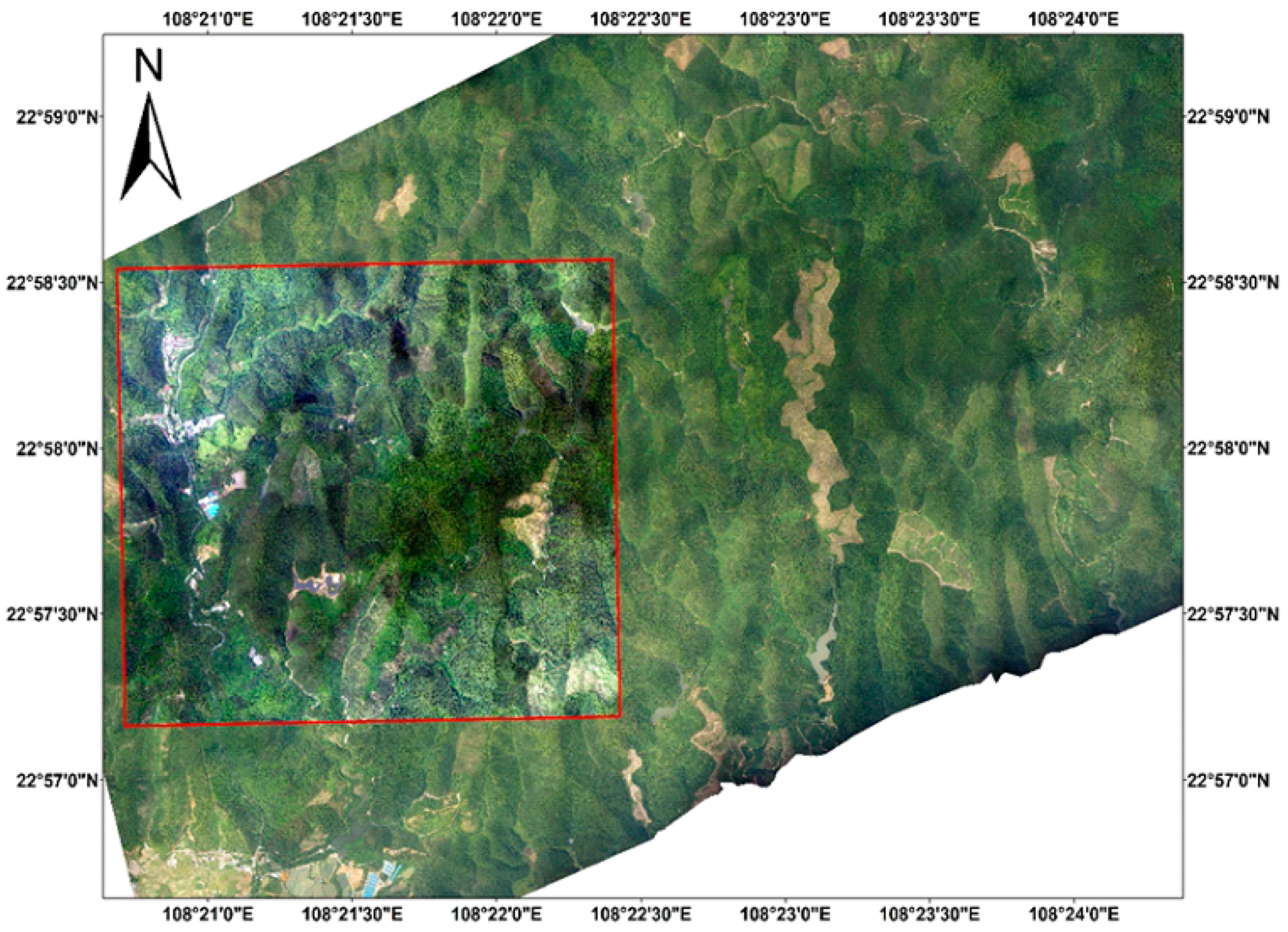
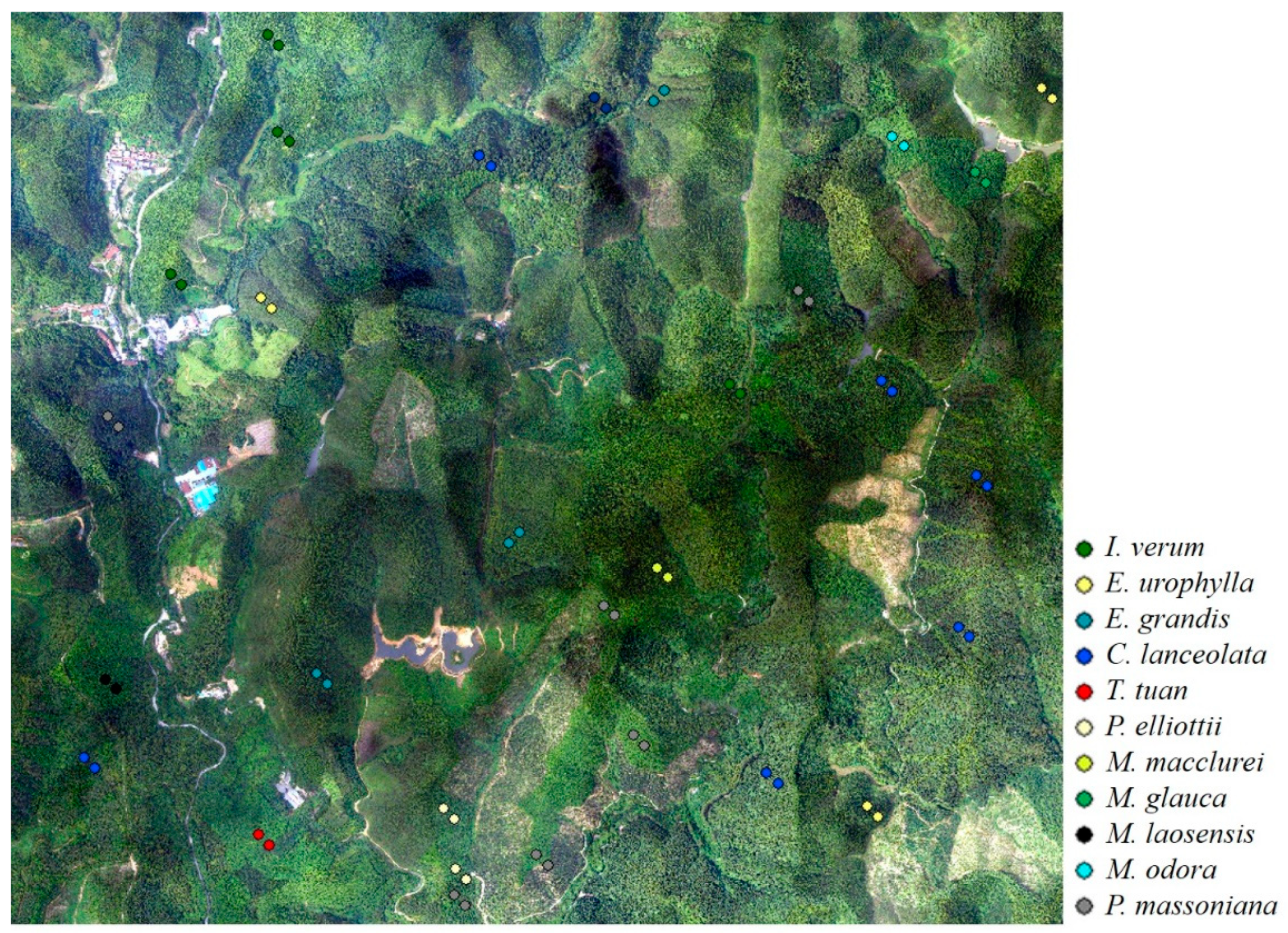
2.1. Study Area

The study area is in the Gaofeng forest farm (22°58′20.54″ N, 108°23′16.26″ E) in Nanning, Guangxi Zhuang Autonomous Region, China (Figure 1). The area, which is in a subtropical monsoon climate zone, is composed of a hilly landform with an elevation varying from 100 to 300 m and a falling gradient of 6° to 35°. The average annual temperature is 21.6 °C, and the annual sunshine time is between 1450 h and 1650 h. Additionally, the annual rainfall, which is mainly concentrated in summer, is 1304.2 mm. The average humidity is above 80%, and the annual evaporation is slightly higher than the rainfall.

This area, with typical characteristics of forests in southern China, is suitable for the growth of a variety of timber trees, especially tropical and subtropical tree species. The forest farm is rich in forest resources, with a forest coverage rate of 87.5%. The number of tree species in the forest mainly includes Eucalyptus robusta Smith, Illicium verum Hook. f., Mytilaria laosensis Lec, Cunninghamia lanceolata, Pinus massoniana Lamb, Pinus elliottii, and other broad-leaved tree species.

2.2. Experimental Data

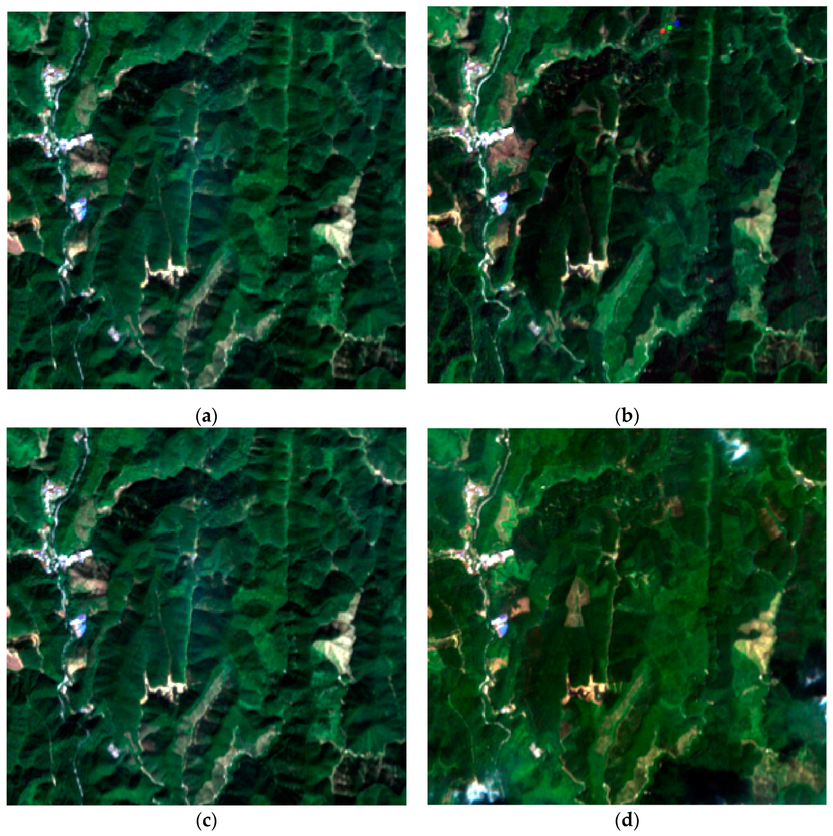
2.2.1. Sentinel-2 Data

Sentinel-2 images are widely available. The multispectral bands of Sentinel-2 images include 13 bands, with bands 2, 3, 4, and 8 having a 10 m spatial resolution; bands 5, 6, 7, 8a, 11, and 12 having a 20 m spatial resolution; and bands 1, 9, and 10 having a 60 m spatial resolution. Due to cloud coverage, only four images which were come from 2015 to 2017 were selected. The four images were acquired on 2 September 2016, 2 June 2016, 1 April 2017, and 30 July 2017, as shown in Figure 2. April and June are the flowering periods of many tree species. In the midsummer in July, the growth of trees is vigorous and leafy. September is the mature period of most trees in the study area. The selected periods are typical time nodes of tree growth, and the spectra of these periods are of equal importance. Time-series multispectral images were stacked in a monthly wise chronological order to provide rich phonological information and spectral–temporal features.

2.2.2. Aerial Image and LiDAR Data

High-resolution aerial images and LiDAR data were acquired by the CAF (The Chinese Academy of Forestry)-LiCHy(LiDAR, Charge-Coupled Device (CCD) and Hyperspectral) airborne remote sensing system platform in June 2016. The LiCHy system, developed by the Chinese Academy of Forestry, includes one full-waveform airborne LiDAR (RIEGL LMS-Q680i) and one high-resolution charge-coupled device camera. The CCD sensor is a DigiCAM-60, and the heading and lateral overlap rates are 60% and 30%, respectively. All sensors share the same position and altitude system [68]. The parameters are shown in

Table 1. The parameters of LiCHy airborne remote sensing system platform.

CCD: DigiCAM-60		LiDAR: Riegl LMS-Q680i
Frame size	8956 × 6708	Wavelength	1550 nm
Pixel size	6 µm	Laser beam divergence	0.5 mrad
Imaging sensor size	40.30 mm × 53.78 mm	Laser pulse length	3 ns
Feld of view (FOV)	56.2°	Cross-track FOV	±30°
Ground resolution @1000 m altitude	0.12 m	Vertical resolution	0.15 m
Focal length	50 mm	Point density @1000 m altitude	3.6 pts/m2
——	——	Waveform Sampling interval	1 ns
——	——	Maximum scanning speed	200 lines/s
——	——	Maximum laser pulse repetition rate	400 kHz

.

2.2.3. Field Data Collection

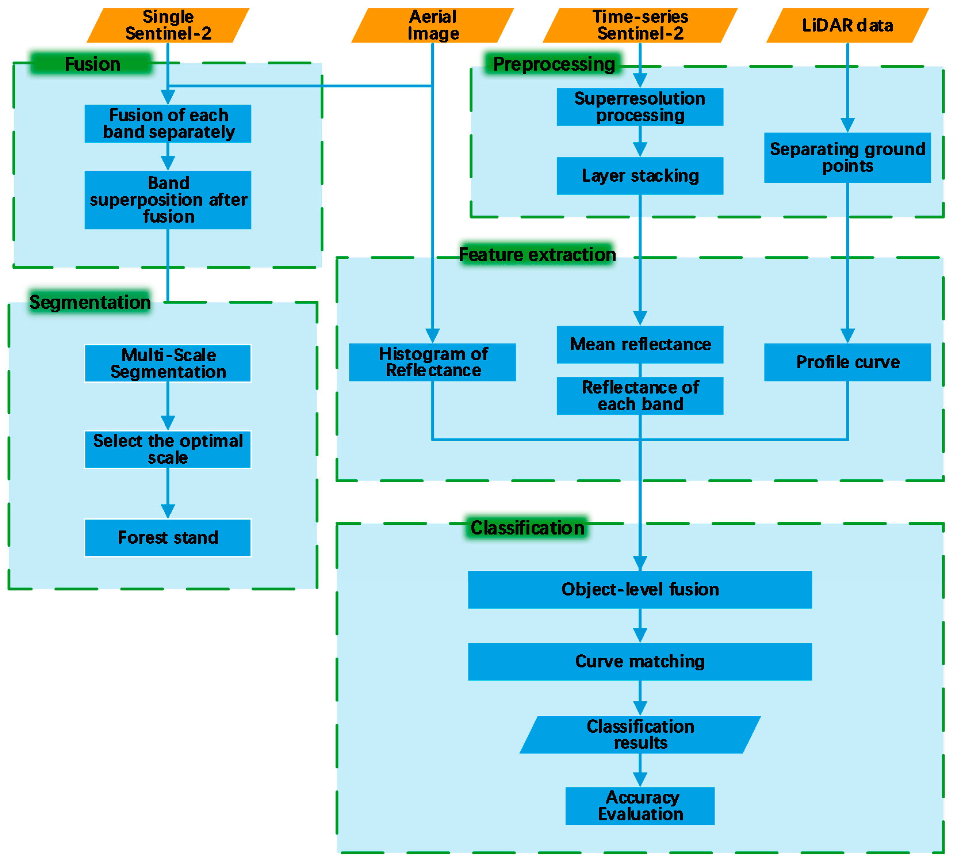
In this study, two types of ground reference data are included: (i) field sampling points and (ii) points interpreted from images. The field sampling plot is a square with a side length of 30 m. The three-dimensional coordinates of the four corner points of the sample plot were measured using dual-frequency differential global positioning system (GPS). The surroundings of forest stands were observed when each plot was sampled. If the forest stands within 30 m around the sampling center were the same tree species, the center was sampled. Otherwise, the center was moved to a suitable place where the sampling plot contained only one tree species. If the sample plot could not contain only one tree species by moving to other places, two tree species can be included. Finally, the coordinates of the four corner points of each sample point, dominant tree species, average breast diameter, and average tree height were recorded.

The field samples were collected in August 2016. The samples include 11s tree species (Illicium verum Hook. f., Eucalyptus urophylla, Eucalyptus grandis, Cunninghamia lanceolata, Linden, Pinus elliottii, Michelia macclurei, Manglietia glauca, Mytilaria laosensis, Tsoongiodendrom odorum, Pinus massoniana) and a total of 30 sampling areas. Figure 3 shows the spatial distribution of all samples, and the range of the sample plot was determined by the diagonal point and its adjacent point. For convenience, all tree species in the following text are abbreviated as shown in

Table 2. Abbreviations of tree species.

Species	Illicium verum	Tilia tuan	Eucalyptus urophylla	Michelia odora
Abbreviation	I. verum	T. tuan	E. urophylla	M. odora
Species	Eucalyptus grandis	Pinus massoniana	Mytilaria laosensis	Cunninghamia lanceolata
Abbreviation	E. grandis	P. massoniana	M. laosensis	C. lanceolata
Species	Manglietia glauca	Michelia macclurei	Pinus elliottii	——
Abbreviation	M. glauca	M. macclurei	P. elliottii	——

. The ratio of training samples to test samples is 1:4 in this study.

2.3. Methods

The flowchart of the FSP method is shown in Figure 4. First, a high-resolution aerial image was fused with a single-time Sentinel-2 image, and the forest stand was obtained by the fractal net evolution approach (FNEA) segmentation. The features of the three types of data were extracted for each forest stand. The histogram was generated using all pixel values in a forest stand (i.e., one segment) for the aerial image across all multispectral bands. The average reflectance of each band was calculated in a forest stand for the time-series images, and the reflectance curve was generated by stacking all the bands of the time-series images. The profile curve of height was generated from the LiDAR data for each forest stand. Finally, the curve matching classifier was applied to classify the forest stands based on the extracted feature curves. The details of the FSP method are described in the following subsections, including data preprocessing, multisource image fusion, forest stand segmentation, feature extraction, and classification.

2.3.1. Data Preprocessing

Atmospheric correction and resampling were applied to the Sentinel-2 image. The Level-1C products of Sentinel-2 images were used. The Sen2Cor plug-in (v255) was used to manually correct the atmosphere on all bands through the Sentinel application platform (SNAP, v6.0.4, available online: http://step.esa.int/main/third-party-plugins-2/sen2cor/). The water vapor band was removed because it mainly reflects the water vapor in the atmosphere. Since multispectral bands of the Sentinel-2 image have different spatial resolutions, a third-party plug-in super-resolution tool Sen2Res was used for resampling. This tool can synthesize all bands with different resolutions to 10 m through super-resolution technology [69].

The LiDAR data were registered with images, and non-signal points were removed. Therefore, the preprocess for the LiDAR data is to classify ground points and forest points. The improved progressive triangulated irregular network (TIN) densification filtering algorithm was applied to classify point clouds [70].

In this algorithm, an appropriate grid size was selected to split the LiDAR data, and the initial grid size was 20 m. The lowest point in each grid was selected as the initial seed point. The seed points were used to construct an initial TIN. To iteratively densify the TIN, all points to be classified were traversed, and the triangles into which the horizontal projection of each point fell were queried. The distance k from the point to the triangle was calculated, and the maximum value of the angle was formed by the point and plane of the triangle. The calculated distance and the angle were compared with the iteration distance (the threshold of the distance was 1.5 m) and iteration angle (the threshold of the value was 8°), respectively. If the distance and angle were less than the thresholds, the point was classified as a ground point and added to the TIN. Thus, the ground points and the points returned from the forest were separated. Finally, the values for these forest points were normalized to 0–1. The final height was obtained by subtracting the digital elevation model (DEM) to remove the influence of terrain.

2.3.2. Multisource Image Fusion

As mentioned before, aerial images have rich textural information, and time-series images contain rich spectral information. The color (spectral) is as important because the texture when using segmentation. Therefore, the Sentinel-2 image obtained on 2 June 2016, was fused with the aerial image since both images were acquired in June. The twelve bands of the Sentinel-2 image were used to fuse with the aerial image. The fusion can make the best use of the spectral and textural information for an accurate segmentation. The fusion method adopted in the experiments was a nonlinear transform and multivariate analysis algorithm (NMV) [71]. The NMV method could minimize the spectral distortion in the fusion image. The steps of the NMV algorithm are described as follows.

(1)

The spatial details were obtained by the difference between the band and its degraded version:

$$M_{i,h}=M_i+M_{i,L}$$

where M_i is the ith band, and M_i,L is an upsampled image using the bicubical method to match the pixel size of the reflective band. The spatial details of the multiple reflective bands can be expressed as follows:

$$M_{i,h,t}={\left(M_i\right)}^t+{(M_{i,L})}^t$$

where t is the coefficient.

(2)

A multivariate regression of a low-resolution image and multiple reflective bands was established.

$$M_{\mathrm{low}}={\displaystyle \sum }_{i=1}^n\left[c_i(M_i{}^t\right)+a_i{M}_i+b+e]$$

where c_i, a_i and b are coefficients; e is the residual; and M_low is the low-spatial-resolution image. Given value t, the coefficients can be estimated using the least squares approach.

(3)

The low-spatial-resolution image was fused to the final image with a high spatial resolution by the following equation:

$$M_{\mathrm{low},f}=M_{\mathrm{low}}+{\displaystyle \sum }_{i=1}^n[c_i{M}_{i,h,t}+a_i{M}_i]$$

2.3.3. Forest Stand Segmentation

The FNEA [72] was applied to segment the forest stand. This algorithm grows from bottom to top, following the principle of minimum heterogeneity and adjacent heterogeneity. Pixels with similar spectral information are merged into a homogenous object, during which the textural, spectral, and shape features of the image object are simultaneously considered. The scale parameter was selected using the automated Estimation of Scale Parameter (ESP2) tool. The scale factor was set to 80. The shape factor was 0.3 and the compactness was 0.1.

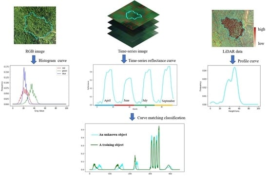
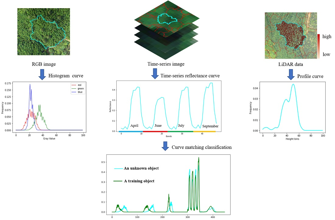
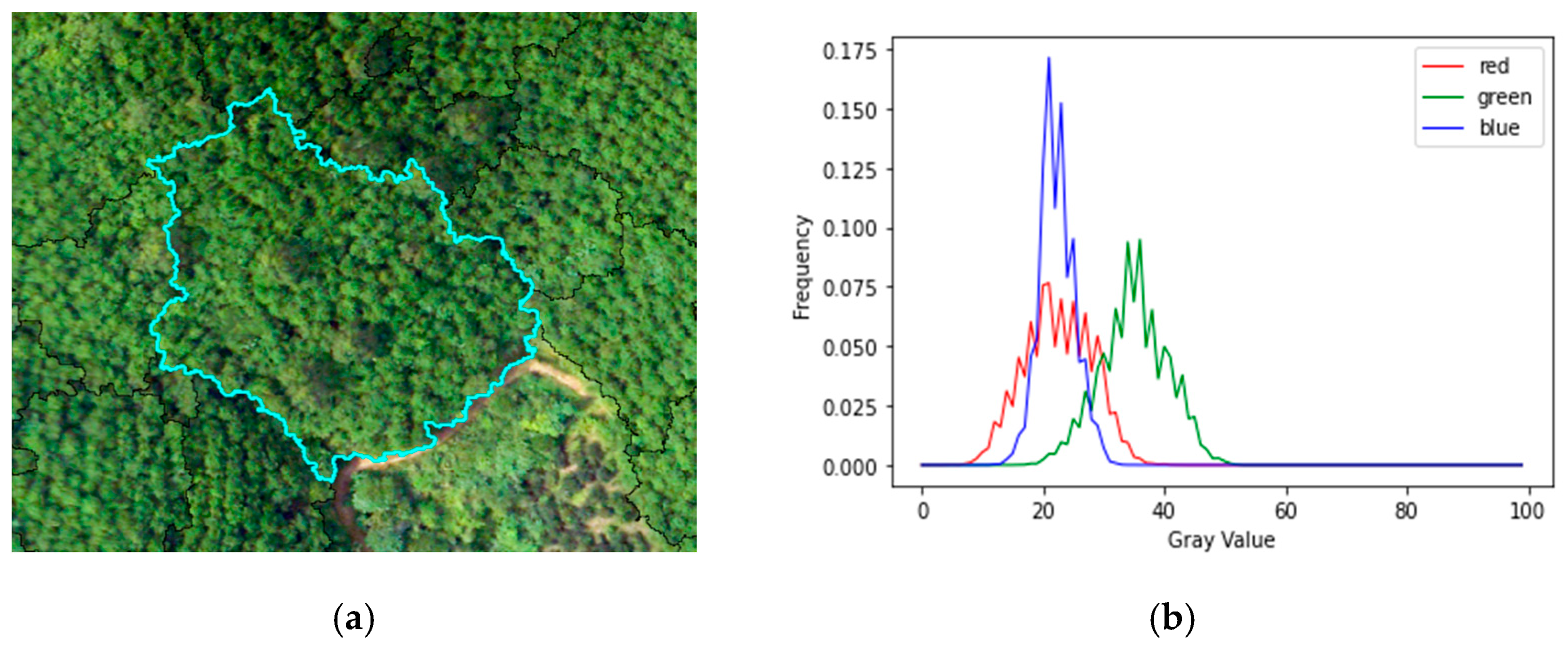
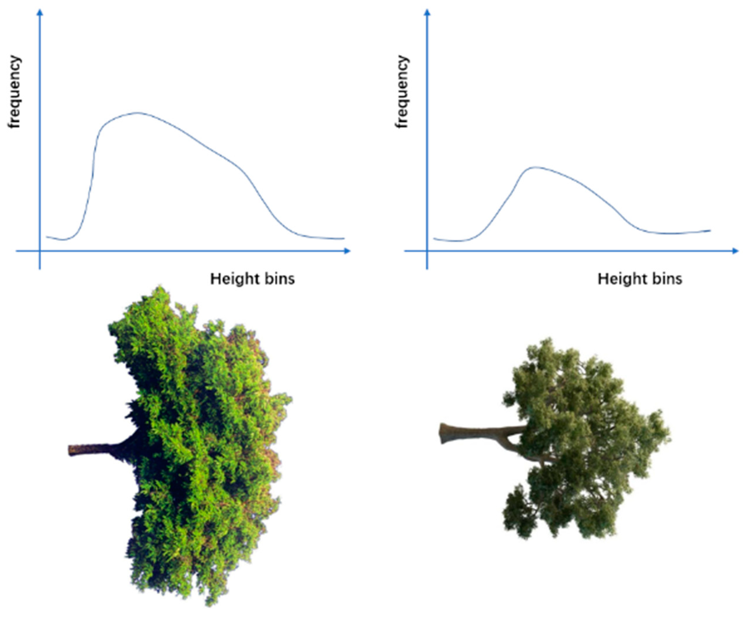
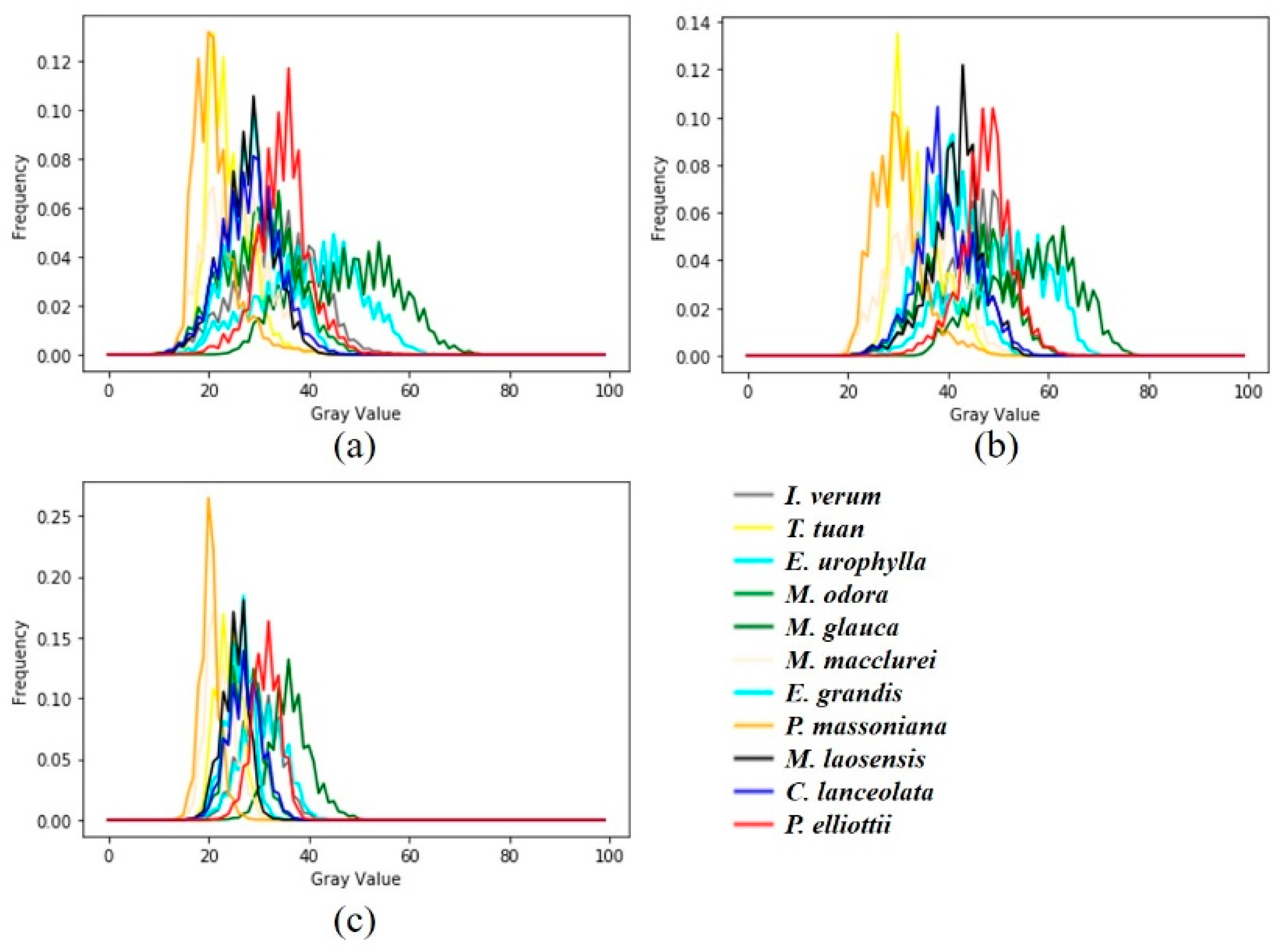
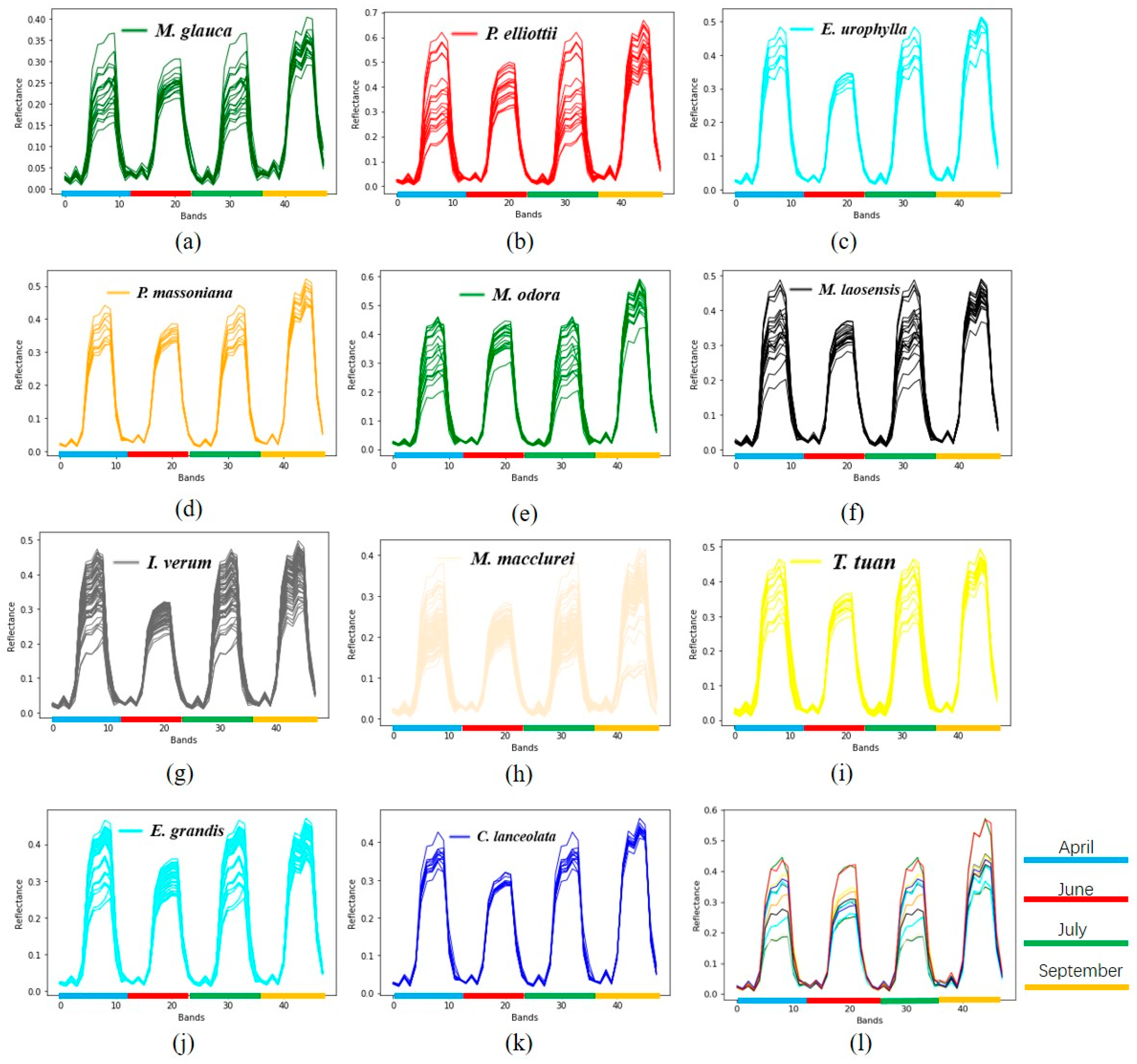
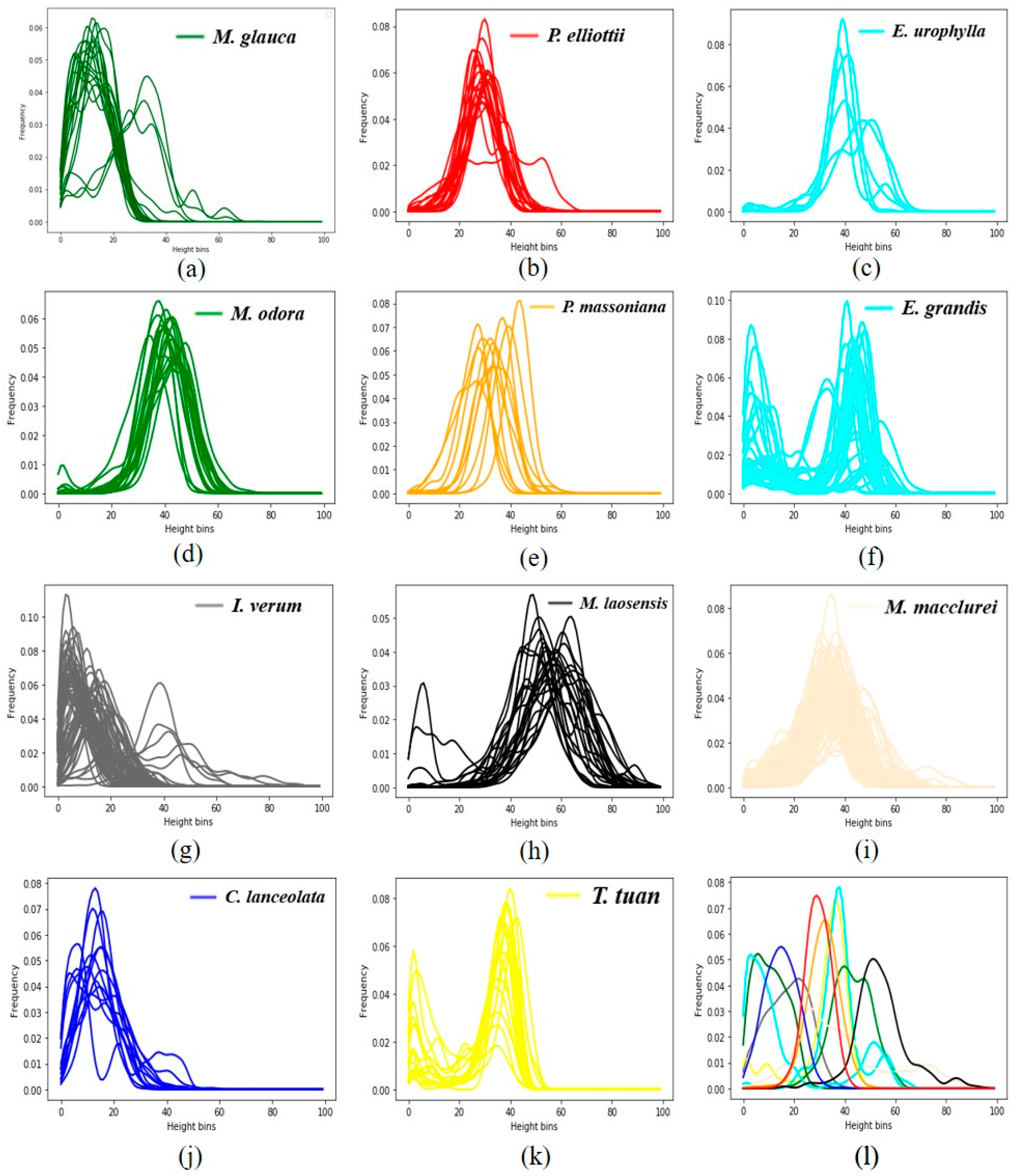
2.3.4. Feature Extraction

By generating the histograms from the aerial image, the brightness of each multispectral band was projected on the x-axis, and the histogram frequency was projected on the y-axis. One hundred histogram bins were set between 0 and 1, and the number of pixels was counted in each bin. Finally, the total number of pixels was used to normalize the generated histogram, so that the effect of different sizes of objects can be eliminated. Figure 5 shows the histograms of a forest stand for three multispectral bands of the aerial image.

The average reflectance of each band for each forest stand was calculated. Figure 6 shows a forest stand for the time-series Sentinel-2 images and the stacked time-series reflectance curve.

For the LiDAR data, the profile curve for each stand was generated to extract the structural features of forest stands. The profile curve was generated from the vertical frequency distribution of the LiDAR data. The profile curve is essentially a histogram of height. Since this curve can characterize the vertical structure of trees, we use the term profile curve. The same tree species have similar structural features, and different tree species have different structural characteristics, as illustrated in Figure 7. Figure 8 shows the profile curve extracted in a forest stand. The steps for generating the profile curve are described as follows. First, the elevation was uniformly discretized, and the value of each elevation interval was calculated. In this study, N was set to 100. The number of point clouds contained in each discrete height interval of each forest stand was calculated, and the vertical profile curve of the point cloud was generated. Finally, after being divided by the total number of point clouds in this forest stand, the profile curve was obtained. The x-axis in Figure 8 is the height bin, and the y-axis is the frequency distribution of the point cloud. The average point number in a stand is 2687, thus the generated curves are rather smooth.

2.3.5. Classification

Five feature curves (three for aerial images, one for time-series images, and one for LiDAR) were extracted for each forest stand. To identify the species that the curves belong to, a fusion method was developed to fuse all features using three curve matching classifiers: The Kullback–Leibler divergence (KL), root sum squared differential area (RSSDA), and curve angle mapper (CAM). In the curve matching classifier, the similarity between the known sample and the sample to be classified was measured. In this study, P1 represents the feature curves of the reference forest stand, and P2 refers to the feature curves of the forest stand to be classified. The three curve matching classifiers are described below.

KL divergence, also known as cross entropy, is a method used to describe the difference between two probability distributions. This method measures the distance between two random distributions. If two random distributions are the same, their relative entropy is zero. As the difference between two random distributions increases, their relative entropy also increases.

$$d_{\mathrm{KL}}={\displaystyle \sum }_i^n\log \left(\frac{P1\left(i\right)}{P2\left(i\right)}\right)P1\left(i\right)$$

CAM calculates the similarity between two discrete curves. The calculation result represents the angle between the curve to be classified and the sample curve in n-dimensional space. The smaller the difference between the two curves, the smaller the angle.

$$d_{\mathrm{CAM}}={\cos }^{-1}\left[\frac{{{\displaystyle \sum }}_{i=1}^{n}P{1}_{i}P{2}_i}{\sqrt{\left({{\displaystyle \sum }}_{i=1}^{n}P{1}_i{}^2\right)}\sqrt{{{\displaystyle \sum }}_{i=1}^{n}P{2}_i{}^2}}\right]$$

RSSDA calculates the difference between the area integrals of two curves. This classifier uses discrete intervals as the differential unit to approximate the area. The RSSDA classifier was originally applied to match spectral curves [73], and was improved by Douglas [74].

$$d_{\mathrm{RSSDA}}=\sqrt{{\displaystyle \sum }_{i=1}^n{\left(P{1}_i-P{2}_i\right)}^2}$$

In Formulas (5)–(7), i is a discrete interval of the curves, and n is the number of intervals. For the histogram of the aerial image, i refers to the ith gray interval of a spectral histogram, n is the number of intervals of this histogram. For the time-series reflectance curve, i refers to the ith band, n is the total number of the stacked bands. For the profile curve, i refers to the ith height bin, n is number of total bins. Moreover, d_KL, d_CAM, d_RSSDA are the similarities of two curves measured using the KL, CAM, RSSDA curve matching methods.

Five feature curves were obtained for each forest stand. For a forest stand to be classified (i.e., a testing sample), its feature curves were compared with the feature curves of all training samples, using one of the above curve matching classifiers. The FSP method is defined as follows:

$$d_{\mathrm{FSP}}=f_1{d}^{\mathrm{R}}+f_2{d}^{\mathrm{G}}+f_3{d}^{\mathrm{B}}+f_4{d}^{\mathrm{TS}}+f_5{d}^{\mathrm{LD}}$$

where f₁, f₂, f₃, f₄, and f₅ are proportional weights for different features. These weights were determined by the controlled variable method. In this study, the weights from f₁ to f₅ were set to 0.2, 0.23, 0.23, 0.1, and 0.24, respectively. Moreover, d^R, d^G, and d^B are the similarities of R, G and B bands of the aerial image, respectively; d^TS is the similarity of time-series image; and d^LD is the similarity of the LiDAR data.

Finally, the maximum value of fusion for each stand to be classified was found, and the category of the training sample corresponding to the maximum value was assigned to the stand to be classified.

3. Results

3.1. The Results of Fusion and Segmentation

Figure 9 shows the fusion results and detailed parts of the aerial image and Sentinel-2 image. These detailed images (Figure 9d) show that textures in the fused image are very clear. The fused image has a high resolution (0.2 m) and richer spectra than the aerial images. The segmentation results and some representative details are shown in Figure 10. As seen in the detailed images, the segmentation results divide the forest stands with different textures, and each forest stand can largely maintain its internal consistency.

3.2. Feature Extraction Results

Figure 11 shows the histograms of 11 tree species in the R, G, and B bands. Figure 12 shows the histograms generated by a single sample for each class in the R, G, and B bands. The histograms in the R and G bands are similar. However, the peak of the R band appears more quickly than the peak of the G band, and the gray value of the B band is more concentrated than the values of the R and G bands. Therefore, the maximum value of the histogram in the B band is larger than that in the R and G bands, and the wave crest appears more quickly in the B band. This similarity can be regarded as the vegetation commonality. In addition to the commonalities, the histogram shapes for different tree species show diversity for different bands. In general, the histograms generated by each category show similarity in the overall distribution. Different categories of tree species have certain differences in each waveband, and some tree species in some wavebands have high degrees of similarity.

Figure 13a–k shows the curves of the time series of eleven tree species. Figure 13l shows the time-series curve generated by a single sample of 11 tree species. In the time-series curves, distinguishability is greatest in the red-edged band (bands 4, 5, 6, and 7), and the spectra show distinctive differences in different seasons.

Figure 14a–k shows the profile curve generated by the LiDAR data for different tree species. The profile curves of the same tree species are similar. This similarity demonstrates that the features extracted from the LiDAR data are effective for distinguishing different tree species. Among the profile curves of 11 tree species, nine have one peak, and two have double peaks. In the curve with two peaks, the first peak is caused by the vegetation under the trees, such as small shrubs. The second peak is caused by the characteristics of trees. When the forest stands are of the same species, the structure below the canopy might be different, which may cause the deviation of the profile curve, such as for M. glauca and I. verum. In addition, the tree species in a forest stand may not be all the same, causing the waveform to deviate. Generally, the amount of deviation in the profile curve is only a small part of the total forest stand.

To clearly show the difference in profile curves among the different tree species, Figure 14l presents the results that integrate the profile curve of different tree species. Generally, different tree species have different waveforms, including the locations of wave peaks and the shape of the waveform. Sometimes, the profile curves of certain tree species are nearly identical, such as P. elliottii and P. massoniana (Figure 14b,e). Therefore, the utilization of the profile curve alone cannot distinguish between P. elliottii and P. massoniana Fortunately, the histograms of P. elliottii and P. massoniana in the R, G, and B bands are distinctive. M. laosensis and C. lanceolata (Figure 14h,j) can be easily distinguished using profile curves even though they have similar histogram and time-series curves.

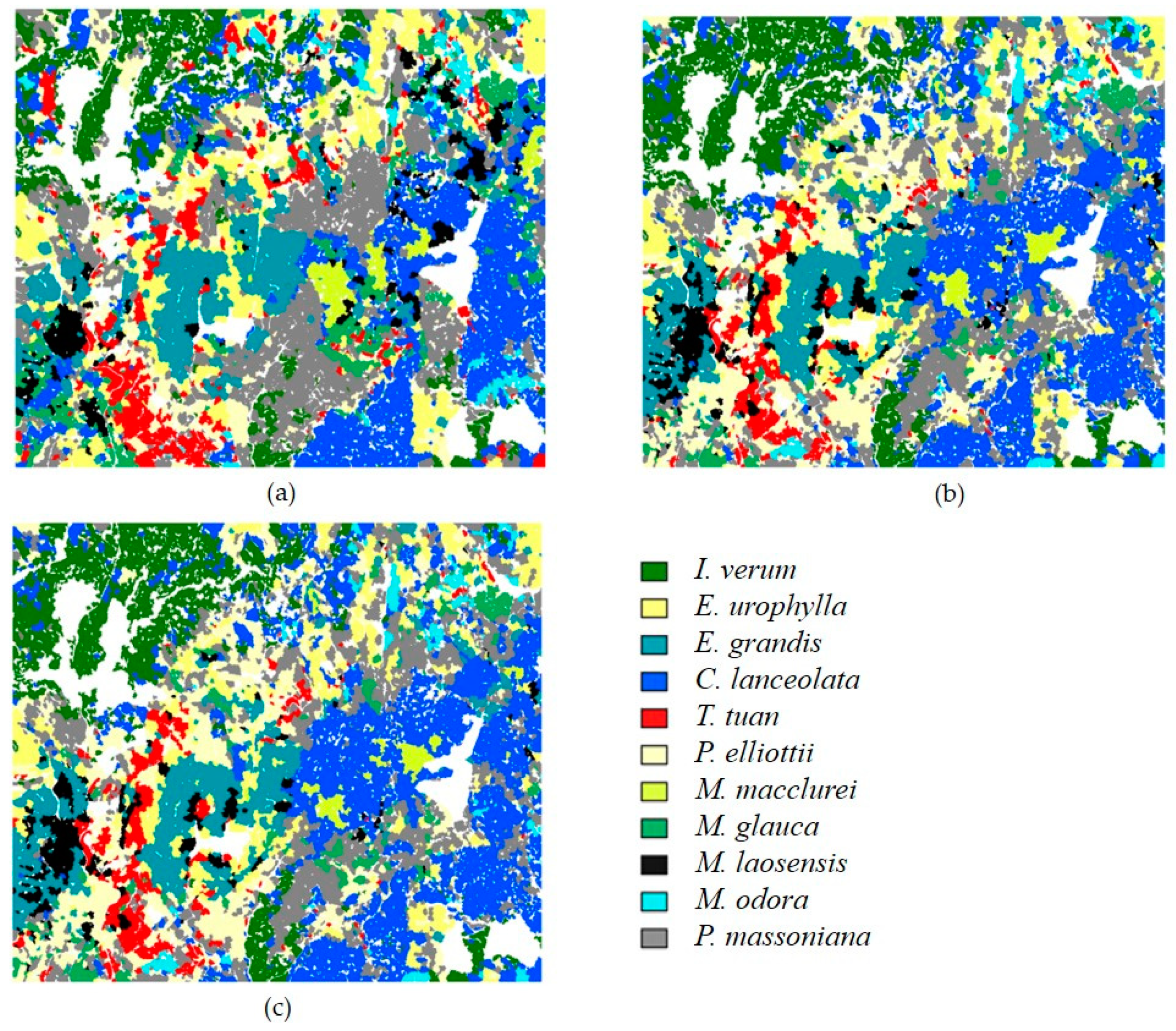
3.3. Classification Results of FSP

Figure 15a shows the classification result obtained using the FSP method KL classifier. The white areas are non-forest areas. C. lanceolata, P. elliottii, I. verum and E. grandis have the widest distributions.

Table 3. Classification accuracies of the FSP method based on the Kullback–Leibler divergence (KL), curve angle mapper (CAM), and root sum squared differential area (RSSDA) curve matching classifiers.

FSP Method	KL-Based			CAM-Based			RSSDA-Based
Class	UA	PA	F1-Score	UA	PA	F1-Score	UA	PA	F1-Score
I. verum	1	0.933	0.966	1	0.867	0.929	0.938	1	0.968
T. tuan	1	1	1	1	0.941	0.970	1	0.824	0.903
E. urophylla	0.818	0.692	0.750	0.800	0.615	0.696	0.909	0.769	0.833
M. odora	1	1	1	1	0.800	0.889	1.000	1	1
M. glauca	1	0.933	0.966	1	0.933	0.966	0.875	0.933	0.903
M. macclurei	1	1	1	0.889	0.889	0.889	1	1	1
E. grandis	0.885	0.920	0.902	0.800	0.960	0.873	0.958	0.920	0.939
P. massoniana	0.980	0.877	0.926	0.942	0.860	0.899	0.943	0.877	0.909
M. laosensis	0.905	1	0.950	0.900	0.947	0.923	1	0.947	0.973
C. lanceolata	0.86	1	0.993	0.932	0.971	0.951	0.920	0.986	0.952
P. elliottii	0.562	0.900	0.692	0.571	0.800	0.667	0.643	0.900	0.750
	Overall accuracy: 0.937 Kappa coefficient: 0.926			Overall accuracy: 0.902 Kappa coefficient: 0.884			Overall accuracy: 0.925 Kappa coefficient: 0.911
UA: user accuracy; PA: product accuracy

shows the classification results using the FSP method based on three curve matching classifiers. The overall accuracy of the KL matching result is 0.937, and the kappa coefficient is 0.926. The overall accuracy of the CAM matching result is 0.902, with a kappa coefficient of 0.884, and the overall accuracy of the RSSDA matching result is 0.925, with a kappa coefficient 0.911. The overall classification results of the FSP methods based on the three curve matching classifiers reach 0.900, and the RSSDA and KL classifiers are better than the CAM. Among all species, E. urophylla and P. elliottii have the worst classification results. The KL and CAM classifiers classify a large part of these two tree species into E. grandis because the two species have greater similarities in the histograms for the R, G and B bands. The product accuracy of P. elliottii is fairly high (0.900), but the user accuracy is poor (0.562) because the number of samples for P. elliottii is small, and the number of samples for P. massoniana is five times more than that of P. elliottii This imbalance of samples caused a part of the P. massoniana to be incorrectly classified as P. elliottii The indices of the FSP method based on three curve matching classifiers indicate that all classifications are well classified except for P. elliottii and E. urophylla However, the F1-score for these two tree species achieves 0.75 and 0.83 in the RSSDA classifier. This test indicates that the FSP method is suited to classify the tree species of forest stands and that the classification accuracy is rather high.

3.4. Comparison between Fusion Results of Different Types of Data

To determine whether the fusion can effectively improve the classification accuracy, we further compared the proposed FSP method with the method based on aerial images alone and the method based on the fusion of aerial images and time-series images. The same curve matching classifiers (KL, CAM, and RSSDA) were used. To reduce the effects of sampling, ten performances were applied with different random samples. The ratio of training samples to test samples is 1:4.

Table 4. The average of overall accuracy for ten performances using the KL, CAM, and RSSDA classifiers.

	Aerial Alone			Fusion of Aerial Image and Time-Series Images			Fusion of Aerial Image, Time-Series Images, and LiDAR Data
	AVG	SD	MAX	AVG	SD	MAX	AVG	SD	MAX
KL	0.795	0.023	0.835	0.805	0.021	0.839	0.911	0.017	0.937
CAM	0.788	0.016	0.808	0.788	0.017	0.812	0.900	0.014	0.925
RSSDA	0.794	0.019	0.820	0.797	0.017	0.824	0.913	0.017	0.945

shows the accuracy of the assessment results. When only the aerial image was used, the average classification accuracies (AVG) of ten performances were 0.795, 0.788, and 0.794 based on KL, CAM, and RSSDA, respectively, and the highest accuracy (MAX) reached 0.835. The fusion of time-series images and aerial images slightly improved the classification accuracy. The classification accuracies of FSP were 0.911, 0.900, and 0.913 based on the KL, CAM, and RSSDA classifiers, respectively. The accuracy of FSP was higher than that of the method that uses only aerial images. The SD column shows the standard deviation of the accuracies for the ten performances. The standard deviation decreased as more data were fused. The standard deviation of FSP was significantly lower than the other two methods, suggesting that the FSP method is more robust and less affected by sampling.

From the results of fusing different types of data in Table 4, it can be seen that the most helpful information for classification mainly comes from the aerial image and LiDAR data. The improvement contributed by the time-series images is limited. Nevertheless, the standard deviation of ten classification results is reduced when introducing time-series images, indicating a more robust result can be obtained.

Figure 15b,c shows the classification results using the KL classifier based on the fusion of the aerial image and time-series images and the aerial image alone. After fusing the time-series images, the details are improved. By comparing these two results, the classification result of FSP provides a more accurate description of the distribution of tree species.

3.5. Comparison with Traditional Methods

The FSP method was also compared with other traditional object-level classifiers, including the random forest (RF) [27], support vector machine (SVM) [75], and eXtreme Gradient Boosting (XGBoost) algorithms [51]. These three classifiers are commonly used. For traditional OBIA methods, the spectral and textural information for each forest stand were used for all bands of the aerial image and time-series images, whereas only the mean and standard deviation of the heights were used for the LiDAR data [7]. The spectral feature includes the mean and standard deviation, and the textural information includes contrast, entropy, homogeneity, angular second moment, dissimilarity, and correlation based on the gray-level co-occurrence matrix (GLCM) [28]. Therefore, the multi-dimensional summarized characteristics of forest stands are obtained. For a fair comparison, all the classifications were performed on the same ten samplings as previously mentioned.

The FSP and the benchmark classifications were coded in Python 3.7. The main package includes scikit-learn and gdal. The results of traditional classification methods are shown in

Table 5. The accuracy assessment of ten performances of support vector machine (SVM), random forest (RF), eXtreme Gradient Boosting (XGBoost).

	Algorithm	AVG	SD	MAX
Traditional methods	SVM	0.814	0.025	0.855
	RF	0.824	0.034	0.875
	XGBoost	0.817	0.025	0.855
FSP	KL	0.911	0.017	0.937
	CAM	0.900	0.014	0.925
	RSSDA	0.913	0.017	0.945

. The worst classification result was SVM (0.814), and the best result was RF (0.824). RF also had the highest classification accuracy in ten performances (0.875); regardless RF has the largest standard deviation of 0.034. The overall accuracy of the FSP was 0.900, which was 0.09 higher than that of the traditional method. The highest classification accuracy of the FSP was 0.06 higher than that of the traditional method. Additionally, the standard deviation of the ten performances shows that the FSP was more stable than traditional methods. In general, the FSP method we proposed has a higher accuracy than the RF, SVM, XGBoost classifiers based on traditional summarized features (i.e. mean, standard deviation, etc.).

To compare the separability of the summarized features used in the traditional classifications and comprehensive features (i.e., feature curves) used in the FSP method, a projection of these two types of features was performed to visualize their separability. The summarized features (120 dimension) include spectral and textual features of images and two height features of LiDAR data. The comprehensive features (448 dimension) consist of all the points on three types of feature curves in the FSP method. The t-SNE tool [76] was used to downscale the extracted features to two dimensions at the best visual aspect. The final visualization results are shown in Figure 16. The red circles mark some points with poor separability. In general, the points characterized by the comprehensive features in the FSP method are more concentrated, even those in the red circle remain aggregated (Figure 16b). In contrast, the summarized features show a confusion of many tree species (Figure 16a). Therefore, the comprehensive features using the FSP method have better separability than the summarized features based on the traditional classification methods.

4. Discussion

The study area is a managed forest, and there are not many mixed forests in this area. Therefore, the classification accuracy can reach over 90% for 11 tree species. If in a mixed forest, the accuracy may be compromised. Some improvements can be made from the following aspects.

First, the histogram curves from high-spatial-resolution image reflect spectral variability of forest stand. However, the histogram is essentially a disorder expression of the pixels, the spatial relationship lies in the forest stand is ignored. Sometimes forest stands belonging to different tree species may have similar spectral histograms but different textural information. Therefore, the rich textural information contained in the high-spatial-resolution image is not fully utilized. Therefore, in the follow-up research, a more sophisticated feature extraction method is expected to extract and incorporate textural information.

Second, the time-series Sentinel-2 images reflect the phenology features. When introducing phenology features, the classification accuracy is improved 1% and the standard deviation of accuracy is reduced comparing with that used the high-spatial-resolution image alone. It is known that the wavelength beyond 2000 nm is distinctive for many tree species [53]. Sentinel-2 images, however, do not cover such a wide wavelength range. If hyperspectral images are available, the FSP method can be applied similarly and probably derive a better result.

Third, the profile curve from LiDAR data is generated by counting the number of point clouds in forest stands, which means that the profile curves greatly rely on the density of point clouds. The shape of the profile curves is also affected by the shape of the tree and the size of the stand area. If in a mixed forest, the density of the point clouds is required to be high to characterize different structures of different tree species in the profile curve.

Finally, if the tree species are mixed seriously, it would be difficult to classify tree species at the forest stand level. Instead, classification can be performed at the individual tree level. In such case, the current FNEA segmentation algorithm is not suited, and the individual tree delineation algorithm is required. The FSP method can be extended to the delineation result, but higher requirements for the spatial resolution of images and the density of the LiDAR data are required to extract distinct features of individual trees.

5. Conclusions

This paper proposed an FSP method to synthesize high-spatial-resolution multispectral images, time-series images, and LiDAR data. The developed FSP method first extracts rich information in the form of curves from three types of data. The histogram for the multispectral band is generated in a stand for the high-spatial-resolution image, the average reflectance is calculated in each stand for a single band of time-series images, and a reflectance curve is generated by stacking time-series bands, and the profile curve from the point cloud LiDAR data is generated for each stand. Then, the fusion method is used based on curve matching classifiers for forest mapping. The performance of the three curve matching classifiers is evaluated, including KL, CAM, and RSSDA.

The features provided by different types of data contain a large amount of key information. The histograms extracted from the aerial image have richer spectral information than those of traditional OBIA methods based on some statistical measures, such as the mean and standard deviation. The phenology information is contained in time-series images and, thus, distinctive features can be reflected for some tree species from the reflectance curves. The profile curve generated from LiDAR data includes rich forest structure information and is effective in distinguishing tree species. Additionally, the features in the form of the curves facilitate the fusion of disparate data on the stand unit by introducing curve matching classifiers. The results show that the FSP method fused with three types of data can achieve higher accuracy and is more stable than the methods fused with less data or using only aerial images. The FSP method also shows a great advantage over traditional OBIA classification methods.

References

1. Schiefer, F.; Kattenborn, T.; Frick, A.; Frey, J.; Schall, P.; Koch, B.; Schmidtlein, S. Mapping forest tree species in high resolution UAV-based RGB-imagery by means of convolutional neural networks. ISPRS J. Photogramm. Remote Sens. 2020, 170, 205–215. [Google Scholar] [CrossRef]
2. Puumalainen, J.; Kennedy, P.; Folving, S. Monitoring forest biodiversity: A European perspective with reference to temperate and boreal forest zone. J. Env. Manag. 2003, 67, 5–14. [Google Scholar] [CrossRef]
3. Ørka, H.O.; Dalponte, M.; Gobakken, T.; Næsset, E.; Ene, L.T. Characterizing forest species composition using multiple remote sensing data sources and inventory approaches. Scand. J. For. Res. 2013, 28, 677–688. [Google Scholar] [CrossRef]
4. Dalponte, M.; Bruzzone, L.; Gianelle, D. Tree species classification in the Southern Alps based on the fusion of very high geometrical resolution multispectral/hyperspectral images and LiDAR data. Remote Sens. Environ. 2012, 123, 258–270. [Google Scholar] [CrossRef]
5. Li, W.K.; Guo, Q.H.; Jakubowski, M.K.; Kelly, M. A New Method for Segmenting Individual Trees from the Lidar Point Cloud. Photogramm. Eng. Remote Sens. 2012, 78, 75–84. [Google Scholar] [CrossRef] [Green Version]
6. Yu, X.W.; Hyyppa, J.; Kaartinen, H.; Maltamo, M. Automatic detection of harvested trees and determination of forest growth using airborne laser scanning. Remote Sens. Environ. 2004, 90, 451–462. [Google Scholar] [CrossRef]
7. Torabzadeh, H.; Leiterer, R.; Hueni, A.; Schaepman, M.E.; Morsdorf, F. Tree species classification in a temperate mixed forest using a combination of imaging spectroscopy and airborne laser scanning. Agric. For. Meteorol. 2019, 279, 107744. [Google Scholar] [CrossRef]
8. Crabbe, R.A.; Lamb, D.; Edwards, C. Discrimination of species composition types of a grazed pasture landscape using Sentinel-1 and Sentinel-2 data. Int. J. Appl. Earth Obs. Geoinf. 2020, 84, 101978. [Google Scholar] [CrossRef]
9. Dechesne, C.; Mallet, C.; Le Bris, A.; Gouet, V.; Hervieu, A. Forest Stand Segmentation Using Airborne Lidar Data and Very High Resolution Multispectral Imagery. ISPRS—Int. Arch. Photogramm. Remote Sens. Spat. Inf. Sci. 2016, XLI-B3, 207–214. [Google Scholar] [CrossRef]
10. Liu, J.; Wang, X.; Wang, T. Classification of tree species and stock volume estimation in ground forest images using Deep Learning. Comput. Electron. Agric. 2019, 166, 105012. [Google Scholar] [CrossRef]
11. Shi, Y.F.; Skidmore, A.K.; Wang, T.J.; Holzwarth, S.; Heiden, U.; Pinnel, N.; Zhu, X.; Heurich, M. Tree species classification using plant functional traits from LiDAR and hyperspectral data. Int. J. Appl. Earth Obs. Geoinf. 2018, 73, 207–219. [Google Scholar] [CrossRef]
12. Lin, Y.; Hyyppä, J. A comprehensive but efficient framework of proposing and validating feature parameters from airborne LiDAR data for tree species classification. Int. J. Appl. Earth Obs. Geoinf. 2016, 46, 45–55. [Google Scholar] [CrossRef]
13. Immitzer, M.; Atzberger, C.; Koukal, T. Tree Species Classification with Random Forest Using Very High Spatial Resolution 8-Band WorldView-2 Satellite Data. Remote Sens. 2012, 4, 2661–2693. [Google Scholar] [CrossRef] [Green Version]
14. Pu, R.; Landry, S. A comparative analysis of high spatial resolution IKONOS and WorldView-2 imagery for mapping urban tree species. Remote Sens. Environ. 2012, 124, 516–533. [Google Scholar] [CrossRef]
15. Wang, K.; Akar, G. Gender gap generators for bike share ridership: Evidence from Citi Bike system in New York City. J. Transp. Geogr. 2019, 76, 1–9. [Google Scholar] [CrossRef]
16. Heinzel, J.; Koch, B. Investigating multiple data sources for tree species classification in temperate forest and use for single tree delineation. Int. J. Appl. Earth Obs. Geoinf. 2012, 18, 101–110. [Google Scholar] [CrossRef]
17. Clark, M.L.; Roberts, D.A. Species-Level Differences in Hyperspectral Metrics among Tropical Rainforest Trees as Determined by a Tree-Based Classifier. Remote Sens. 2012, 4, 1820–1855. [Google Scholar] [CrossRef] [Green Version]
18. Pu, R.; Landry, S. Mapping urban tree species by integrating multi-seasonal high resolution pléiades satellite imagery with airborne LiDAR data. Urban For. Urban Green. 2020, 53, 126675. [Google Scholar] [CrossRef]
19. Asner, G.P.; Martin, R.E. Airborne spectranomics: Mapping canopy chemical and taxonomic diversity in tropical forests. Front. Ecol. Environ. 2009, 7, 269–276. [Google Scholar] [CrossRef] [Green Version]
20. Nagendra, H. Using remote sensing to assess biodiversity. Int. J. Remote Sens. 2010, 22, 2377–2400. [Google Scholar] [CrossRef]
21. Wolter, P.T.; Mladenoff, D.J.; Host, G.E.; Crow, T.R. Improved Forest stamped classification in the northern lake states using multi-temporal Landsat imagery. Photogramm. Eng. Remote Sens. 1995, 61, 1129–1143. [Google Scholar]
22. Mead, R.A. LANDSAT Digital Data Application to Forest Vegetation and Land Use Classification in Minnesota; Purdue University: West Lafayette, IN, USA, 1977. [Google Scholar]
23. Roller, N.E.G.; Visser, L. Accuracy of landsat forest cover type mapping. Cell Biol. Int. 1994, 18, 289–290. [Google Scholar]
24. Johansen, K.; Phinn, S. Mapping structural parameters and species composition of riparian vegetation using IKONOS and landsat ETM plus data in Australian tropical savannahs. Photogramm. Eng. Remote Sens. 2006, 72, 71–80. [Google Scholar] [CrossRef]
25. Mallinis, G.; Koutsias, N.; Tsakiri-Strati, M.; Karteris, M. Object-based classification using Quickbird imagery for delineating forest vegetation polygons in a Mediterranean test site. ISPRS J. Photogramm. Remote Sens. 2008, 63, 237–250. [Google Scholar] [CrossRef]
26. Huang, W.; Li, H.; Lin, G. Classifying Forest Stands Based on Multi-Scale Structure Features Using Quickbird Image. In Proceedings of the 2015 2nd IEEE International Conference on Spatial Data Mining and Geographical Knowledge Services, Fuzhou, China, 8–10 July 2015; pp. 202–208. [Google Scholar]
27. Karlson, M.; Ostwald, M.; Reese, H.; Bazié, H.R.; Tankoano, B. Assessing the potential of multi-seasonal WorldView-2 imagery for mapping West African agroforestry tree species. Int. J. Appl. Earth Obs. Geoinf. 2016, 50, 80–88. [Google Scholar] [CrossRef]
28. Michez, A.; Piegay, H.; Lisein, J.; Claessens, H.; Lejeune, P. Classification of riparian forest species and health condition using multi-temporal and hyperspatial imagery from unmanned aerial system. Env. Monit. Assess. 2016, 188, 146. [Google Scholar] [CrossRef] [PubMed] [Green Version]
29. Ferreira, M.P.; Wagner, F.H.; Aragão, L.E.O.C.; Shimabukuro, Y.E.; de Souza Filho, C.R. Tree species classification in tropical forests using visible to shortwave infrared WorldView-3 images and texture analysis. ISPRS J. Photogramm. Remote Sens. 2019, 149, 119–131. [Google Scholar] [CrossRef]
30. Yu, Q.; Gong, P.; Clinton, N.; Biging, G.; Kelly, M.; Schirokauer, D. Object-based Detailed Vegetation Classification with Airborne High Spatial Resolution Remote Sensing Imagery. Photogramm. Eng. Remote Sens. 2006, 72, 799–811. [Google Scholar] [CrossRef] [Green Version]
31. Franklin, S.E.; Ahmed, O.S. Deciduous tree species classification using object-based analysis and machine learning with unmanned aerial vehicle multispectral data. Int. J. Remote Sens. 2017, 39, 5236–5245. [Google Scholar] [CrossRef]
32. Zhou, Y.H.; Qiu, F. Fusion of high spatial resolution WorldView-2 imagery and LiDAR pseudo-waveform for object-based image analysis. ISPRS J. Photogramm. Remote Sens. 2015, 101, 221–232. [Google Scholar] [CrossRef]
33. Tang, Y.; Qiu, F.; Jing, L.; Shi, F.; Li, X. Integrating spectral variability and spatial distribution for object-based image analysis using curve matching approaches. ISPRS J. Photogramm. Remote Sens. 2020, 169, 320–336. [Google Scholar] [CrossRef]
34. Madonsela, S.; Cho, M.A.; Mathieu, R.; Mutanga, O.; Ramoelo, A.; Kaszta, Ż.; Kerchove, R.V.D.; Wolff, E. Multi-phenology WorldView-2 imagery improves remote sensing of savannah tree species. Int. J. Appl. Earth Obs. Geoinf. 2017, 58, 65–73. [Google Scholar] [CrossRef] [Green Version]
35. Pu, R.; Landry, S.; Yu, Q. Assessing the potential of multi-seasonal high resolution Pléiades satellite imagery for mapping urban tree species. Int. J. Appl. Earth Obs. Geoinf. 2018, 71, 144–158. [Google Scholar] [CrossRef]
36. Cochrane, M.A. Using vegetation reflectance variability for species level classification of hyperspectral data. Int. J. Remote Sens. 2010, 21, 2075–2087. [Google Scholar] [CrossRef]
37. Ustin, S.L.; Roberts, D.A.; Gamon, J.A.; Asner, G.P.; Green, R.O. Using imaging spectroscopy to study ecosystem processes and properties. Bioscience 2004, 54, 523–534. [Google Scholar] [CrossRef]
38. Fasnacht, L.; Renard, P.; Brunner, P. Robust input layer for neural networks for hyperspectral classification of data with missing bands. Appl. Comput. Geosci. 2020, 8, 100034. [Google Scholar] [CrossRef]
39. Zhao, Q.; Jia, S.; Li, Y. Hyperspectral remote sensing image classification based on tighter random projection with minimal intra-class variance algorithm. Pattern Recognit. 2021, 111, 107635. [Google Scholar] [CrossRef]
40. Li, W.; Du, Q.; Xiong, M. Kernel Collaborative Representation With Tikhonov Regularization for Hyperspectral Image Classification. IEEE Geosci. Remote Sens. Lett. 2014, 12, 48–52. [Google Scholar]
41. Lixin, G.; Weixin, X.; Jihong, P. Segmented minimum noise fraction transformation for efficient feature extraction of hyperspectral images. Pattern Recognit. 2015, 48, 3216–3226. [Google Scholar] [CrossRef]
42. Dalponte, M.; Bruzzone, L.; Gianelle, D. Fusion of hyperspectral and LIDAR remote sensing data for classification of complex forest areas. IEEE Trans. Geosci. Remote Sens. 2008, 46, 1416–1427. [Google Scholar] [CrossRef] [Green Version]
43. Jones, T.G.; Coops, N.C.; Sharma, T. Assessing the utility of airborne hyperspectral and LiDAR data for species distribution mapping in the coastal Pacific Northwest, Canada. Remote Sens. Environ. 2010, 114, 2841–2852. [Google Scholar] [CrossRef]
44. Morsdorf, F.; Meier, E.; Kotz, B.; Itten, K.I.; Dobbertin, M.; Allgower, B. LIDAR-based geometric reconstruction of boreal type forest stands at single tree level for forest and wildland fire management. Remote Sens. Environ. 2004, 92, 353–362. [Google Scholar] [CrossRef]
45. Vauhkonen, J.; Ørka, H.O.; Holmgren, J.; Dalponte, M.; Heinzel, J.; Koch, B. Tree Species Recognition Based on Airborne Laser Scanning and Complementary Data Sources. In Forestry Applications of Airborne Laser Scanning; Springer: Berlin/Heidelberg, Germany, 2014; pp. 135–156. [Google Scholar]
46. Ke, Y.H.; Quackenbush, L.J.; Im, J. Synergistic use of QuickBird multispectral imagery and LIDAR data for object-based forest species classification. Remote Sens. Environ. 2010, 114, 1141–1154. [Google Scholar] [CrossRef]
47. Nilsson, M.; Nordkvist, K.; Jonzén, J.; Lindgren, N.; Axensten, P.; Wallerman, J.; Egberth, M.; Larsson, S.; Nilsson, L.; Eriksson, J.; et al. A nationwide forest attribute map of Sweden predicted using airborne laser scanning data and field data from the National Forest Inventory. Remote Sens. Environ. 2017, 194, 447–454. [Google Scholar] [CrossRef]
48. Popescu, S.C.; Wynne, R.H.; Nelson, R.F. Measuring individual tree crown diameter with lidar and assessing its influence on estimating forest volume and biomass. Can. J. Remote Sens. 2003, 29, 564–577. [Google Scholar] [CrossRef]
49. Morsdorf, F.; Kotz, B.; Meier, E.; Itten, K.I.; Allgower, B. Estimation of LAI and fractional cover from small footprint airborne laser scanning data based on gap fraction. Remote Sens. Environ. 2006, 104, 50–61. [Google Scholar] [CrossRef]
50. Piiroinen, R.; Fassnacht, F.E.; Heiskanen, J.; Maeda, E.; Mack, B.; Pellikka, P. Invasive tree species detection in the Eastern Arc Mountains biodiversity hotspot using one class classification. Remote Sens. Environ. 2018, 218, 119–131. [Google Scholar] [CrossRef]
51. Karasiak, N.; Sheeren, D.; Fauvel, M.; Willm, J.; Monteil, C. Mapping tree species of forests in southwest France using Sentinel-2 image time series. In Proceedings of the 2017 9th International Workshop on the Analysis of Multitemporal Remote Sensing Images, Brugge, Belgium, 27–29 June 2017. [Google Scholar]
52. Shi, Y.; Wang, T.; Skidmore, A.K.; Heurich, M. Important LiDAR metrics for discriminating forest tree species in Central Europe. ISPRS J. Photogramm. Remote Sens. 2018, 137, 163–174. [Google Scholar] [CrossRef]
53. Fassnacht, F.E.; Latifi, H.; Sterenczak, K.; Modzelewska, A.; Lefsky, M.; Waser, L.T.; Straub, C.; Ghosh, A. Review of studies on tree species classification from remotely sensed data. Remote Sens. Environ. 2016, 186, 64–87. [Google Scholar] [CrossRef]
54. Plourde, L.C.; Ollinger, S.V.; Smith, M.L.; Martin, M.E. Martin. Estimating Species Abundance in a Northern Temperate Forest Using Spectral Mixture Analysis. Photogramm. Eng. Remote Sens. 2007, 73, 829–840. [Google Scholar] [CrossRef] [Green Version]
55. Andrew, M.E.; Ustin, S.L. Habitat suitability modelling of an invasive plant with advanced remote sensing data. Divers. Distrib. 2009, 15, 627–640. [Google Scholar] [CrossRef]
56. Lucas, R.M.; Lee, A.C.; Bunting, P.J. Retrieving forest biomass through integration of CASI and LiDAR data. Int. J. Remote Sens. 2008, 29, 1553–1577. [Google Scholar] [CrossRef]
57. Asner, G.P.; Knapp, D.E.; Kennedy-Bowdoin, T.; Jones, M.O.; Martin, R.E.; Boardman, J.; Hughes, R.F. Invasive species detection in Hawaiian rainforests using airborne imaging spectroscopy and LiDAR. Remote Sens. Environ. 2008, 112, 1942–1955. [Google Scholar] [CrossRef]
58. Hill, R.A.; Thomson, A.G. Mapping woodland species composition and structure using airborne spectral and LiDAR data. Int. J. Remote Sens. 2011, 26, 3763–3779. [Google Scholar] [CrossRef]
59. Naidoo, L.; Cho, M.A.; Mathieu, R.; Asner, G. Classification of savanna tree species, in the Greater Kruger National Park region, by integrating hyperspectral and LiDAR data in a Random Forest data mining environment. ISPRS J. Photogramm. Remote Sens. 2012, 69, 167–179. [Google Scholar] [CrossRef]
60. Hudak, A.T.; Evans, J.S.; Smith, A.M.S. LiDAR Utility for Natural Resource Managers. Remote Sens. 2009, 1, 934–951. [Google Scholar] [CrossRef] [Green Version]
61. Machala, M.; Zejdová, L. Forest Mapping Through Object-based Image Analysis of Multispectral and LiDAR Aerial Data. Eur. J. Remote Sens. 2017, 47, 117–131. [Google Scholar] [CrossRef]
62. Sridharan, H.; Qiu, F. Developing an Object-based Hyperspatial Image Classifier with a Case Study Using WorldView-2 Data. Photogramm. Eng. Remote Sens. 2013, 79, 1027–1036. [Google Scholar] [CrossRef]
63. Blair, J.B.; Hofton, M.A. Modeling laser altimeter return waveforms over complex vegetation using high-resolution elevation data. Geophys. Res. Lett. 1999, 26, 2509–2512. [Google Scholar] [CrossRef]
64. Lovell, J.L.; Jupp, D.L.B.; Culvenor, D.S.; Coops, N.C. Using airborne and ground-based ranging lidar to measure canopy structure in Australian forests. Can. J. Remote Sens. 2003, 29, 607–622. [Google Scholar] [CrossRef]
65. Farid, A.; Goodrich, D.C.; Bryant, R.; Sorooshian, S. Using airborne lidar to predict Leaf Area Index in cottonwood trees and refine riparian water-use estimates. J. Arid Environ. 2008, 72, 1–15. [Google Scholar] [CrossRef] [Green Version]
66. Muss, J.D.; Mladenoff, D.J.; Townsend, P.A. A pseudo-waveform technique to assess forest structure using discrete lidar data. Remote Sens. Environ. 2011, 115, 824–835. [Google Scholar] [CrossRef]
67. Popescu, S.C.; Zhao, K.G.; Neuenschwander, A.; Lin, C.S. Satellite lidar vs. small footprint airborne lidar: Comparing the accuracy of aboveground biomass estimates and forest structure metrics at footprint level. Remote Sens. Environ. 2011, 115, 2786–2797. [Google Scholar] [CrossRef]
68. Pang, Y.; Li, Z.Y.; Ju, H.B.; Lu, H.; Jia, W.; Si, L.; Guo, Y.; Liu, Q.W.; Li, S.M.; Liu, L.X.; et al. LiCHy: The CAF’s LiDAR, CCD and Hyperspectral Integrated Airborne Observation System. Remote Sens. 2016, 8, 398. [Google Scholar] [CrossRef] [Green Version]
69. Brodu, N. Super-Resolving Multiresolution Images With Band-Independent Geometry of Multispectral Pixels. IEEE Trans. Geosci. Remote Sens. 2017, 55, 4610–4617. [Google Scholar] [CrossRef] [Green Version]
70. Zhao, X.Q.; Guo, Q.H.; Su, Y.J.; Xue, B.L. Improved progressive TIN densification filtering algorithm for airborne LiDAR data in forested areas. ISPRS J. Photogramm. Remote Sens. 2016, 117, 79–91. [Google Scholar] [CrossRef] [Green Version]
71. Jing, L.H.; Cheng, Q.M. A technique based on non-linear transform and multivariate analysis to merge thermal infrared data and higher-resolution multispectral data. Int. J. Remote Sens. 2010, 31, 6459–6471. [Google Scholar] [CrossRef]
72. Schäpe, M.B.A. Multiresolution Segmentation: An optimization approach for high quality multi-scale image segmentation. In Beutrage zum AGIT-Symposium. Salzburg, Heidelberg; Wichmann: Lotte, Germany, 2000; pp. 12–23. [Google Scholar]
73. Hamada, Y.; Stow, D.A.; Coulter, L.L.; Jafolla, J.C.; Hendricks, L.W. Detecting Tamarisk species (Tamarix spp.) in riparian habitats of Southern California using high spatial resolution hyperspectral imagery. Remote Sens. Environ. 2007, 109, 237–248. [Google Scholar] [CrossRef]
74. Stow, D.A.; Toure, S.I.; Lippitt, C.D.; Lippitt, C.L.; Lee, C.R. Frequency distribution signatures and classification of within-object pixels. Int. J. Appl. Earth Obs. Geoinf. 2012, 15, 49–56. [Google Scholar] [CrossRef] [Green Version]
75. Wessel, M.; Brandmeier, M.; Tiede, D. Evaluation of Different Machine Learning Algorithms for Scalable Classification of Tree Types and Tree Species Based on Sentinel-2 Data. Remote Sens. 2018, 10, 1419. [Google Scholar] [CrossRef] [Green Version]
76. Diamand, M. The Solution to Overpopulation, The Depletion of Resources and Global Warming. J. Neurol. Neurosci. 2016, 7, 140. [Google Scholar] [CrossRef]
Figure 1. The study site in Gaofeng forest farm, Nanning, Guangxi Zhuang Autonomous Region, China.
Remotesensing 13 00144 g001
Figure 2. Time-series Sentinel-2 images: (a) 1 April 2017; (b) 2 June 2016; (c) 30 July 2017; (d) 2 September 2016.
Remotesensing 13 00144 g002
Figure 3. Distribution of sample points.
Remotesensing 13 00144 g003
Figure 4. The flowchart of the fusion of spectral image and point data (FSP) method.
Remotesensing 13 00144 g004
Figure 5. Grayscale histogram generated from aerial image of a forest stand. (a) A forest stand. (b) The histogram of the forest stand in bands R, G, and B.
Remotesensing 13 00144 g005
Figure 6. The reflectance curve of time-series image of a forest stand. (a) A forest stand. (b) The average reflectance of a forest stand for each band. (c) The reflectance curve across the stacked time-series bands.
Remotesensing 13 00144 g006
Figure 7. The profile curve in the vertical direction with different characteristics of a tree’s spatial structure.
Remotesensing 13 00144 g007
Figure 8. Frequency distribution map generated from light detection and ranging (LiDAR) data of a forest stand. (a) A forest stand and the LiDAR data. (b) The profile curve of the forest stand.
Remotesensing 13 00144 g008
Figure 9. The relative image of fusion. (a) Aerial image. (b) Sentinel-2 image. (c) The results of Sentinel-2 image fused with aerial image. (d) The details of fusion results. The left part is the Sentinel-2 image; the right part shows the image after fusion.
Remotesensing 13 00144 g009
Figure 10. The results of segmentation and the enlarged details.
Remotesensing 13 00144 g010
Figure 11. The histograms of 11 tree species in the R, G, B bands.
Remotesensing 13 00144 g011
Figure 12. The histograms generated in the R, G, B, bands of 11 types of tree species. (a) The histograms in the R band. (b) The histograms in the G band. (c) The histograms in the B band.
Remotesensing 13 00144 g012
Figure 13. (ak) The spectral curve of time-series image of 11 tree species, and (l) a comparison chart of the curves for 11 tree species, shows the curves of the time series of eleven tree species.
Remotesensing 13 00144 g013
Figure 14. (ak) The profile curve generated by the LiDAR data of 11 tree species and (l) a comparison chart of the curves for 11 tree species.
Remotesensing 13 00144 g014
Figure 15. The classification results of three methods. (a) The FSP result based on KL. (b) The results using aerial and time-series image based on KL. (c) The results of using aerial image alone based on KL.
Remotesensing 13 00144 g015
Figure 16. Separability of features: (a) the separability of summarized features used in traditional methods. (b) The separability of comprehensive features used in the FSP method.
Remotesensing 13 00144 g016