Article

Hyperspectral Image Classification Based on Multi-Scale Residual Network with Attention Mechanism

School of Instrument and Electronics, North University of China, Taiyuan 030000, China
*
Author to whom correspondence should be addressed.
Remote Sens. 2021, 13(3), 335; https://doi.org/10.3390/rs13030335
Submission received: 21 December 2020 / Revised: 15 January 2021 / Accepted: 16 January 2021 / Published: 20 January 2021

Abstract

:
In recent years, image classification on hyperspectral imagery utilizing deep learning algorithms has attained good results. Thus, spurred by that finding and to further improve the deep learning classification accuracy, we propose a multi-scale residual convolutional neural network model fused with an efficient channel attention network (MRA-NET) that is appropriate for hyperspectral image classification. The suggested technique comprises a multi-staged architecture, where initially the spectral information of the hyperspectral image is reduced into a two-dimensional tensor, utilizing a principal component analysis (PCA) scheme. Then, the constructed low-dimensional image is input to our proposed ECA-NET deep network, which exploits the advantages of its core components, i.e., multi-scale residual structure and attention mechanisms. We evaluate the performance of the proposed MRA-NET on three public available hyperspectral datasets and demonstrate that, overall, the classification accuracy of our method is 99.82 %, 99.81%, and 99.37, respectively, which is higher compared to the corresponding accuracy of current networks such as 3D convolutional neural network (CNN), three-dimensional residual convolution structure (RES-3D-CNN), and space–spectrum joint deep network (SSRN).

Graphical Abstract

1. Introduction

A hyperspectral image presents a target region in a spectrum of continuous and narrow bands, containing both spatial and spectral feature information at a pixel-level resolution [1]. Hyperspectral imagery is widely used in various applications such as urban planning, agricultural development, and environmental testing [2]. Technically, a hyperspectral image is a three-dimensional image composed of an image along several spectral dimensions. The analysis of a hyperspectral image’s spatial and spectral characteristics can effectively contribute to the classification of ground objects. However, hyperspectral images are prone to the Hughes phenomenon due to the complexity of their structure and suffer from a small number of labeled samples affecting the overall performance of hyperspectral image classification. Due to these deficiencies, hyperspectral image classification still poses a hot research topic.
Thus, the literature presents several attempts toward hyperspectral image classification. For example, traditional classifiers are utilized such as the support vector machine (SVM), K-nearest neighbor algorithm, and multinomial logistic regression (MLR) [3,4,5,6]. These algorithms mainly exploit the spectral information of the image due to its high dimensionality. Principal component analysis (PCA), independent component analysis (ICA), and image sparse representation (SR) methods are also used to process the spectral information, by extracting its main features and reducing computational complexity [7,8,9,10,11]. However, as opposed to deep learning networks, these traditional methods are not able to extract deep-level features, imposing a relatively low classification accuracy. The deep learning method can extract the abstract-level information of the image, so it is more effective to deal with the hyperspectral classification problem. Indeed, literature offers several deep-learning-based hyperspectral image-classification solutions. In [12], the authors propose a stacked autoencoder (SAE), while the work of [13] presents a convolutional neural network (CNN) architecture appropriate for hyperspectral image classification. Both methods have improved the accuracy of hyperspectral classification compared to the classic computer vision type of approaches presented earlier. Further attempts utilizing deep networks involve a two-dimensional CNN (Conv2D-CNN) to extract spectral–spatial feature information, combined with an image dimensionality reduction algorithm [14,15]. To extract better spatial and spectral features, [16,17,18] use 3D convolution to extract hyperspectral image features, and [19,20,21] fuse a residual with an attention deep network. Methods such as attention mechanism [22] and joint space–spectral features [23] that improve the convolutional neural network classification accuracy and also increase the number of the network parameters have also been used. Finally, in [24] the authors utilize the method of generative adversarial networks (GANs), in [25] the transfer learning technique, in [26] 2D and 3D convolutions, respectively, in [27,28,29] multi-scale adaptive feature extraction, combine these methods with hyperspectral classification problems to further improve the hyperspectral image classification performance.
However, even though all these methods have achieved an acceptable classification performance, the classification accuracy still needs to be further improved. Spurred by that, this paper proposes a multi-scale residual convolutional neural network that integrates an attention mechanism, embeds the lightweight and improved channel attention mechanism proposed by Wang et al. [30], i.e., the efficient channel attention network (ECA-NET), and uses local cross-channel interaction without dimensionality reduction. This strategy, through the adaptive one-dimensional convolution, effectively extracts the spatial and spectral features of the image and reduces the redundancy of the training sample information. Convolutional kernels with different scales and sizes are used along with a novel residual structure, and the space–spectrum features of the image are extracted multiple times. Overfitting is effectively prevented by employing within our deep learning model regularization and smoothing normalization strategies on multiple layers. Experiments on the Pavia University (UP), Kennedy Space Center (KSC), and Indian Pines(IN) datasets highlight the appealing classification performance of our method.
The remaining part of the paper is organized as follows: Section 2 presents the suggested deep learning hyperspectral image-classification strategy, while Section 3 demonstrates the classification capabilities of our method on three datasets. Finally, Section 4 concludes this paper.

2. Multi-Scale Residual Network Model Integrating Attention Mechanism

Hyperspectral images present high spectral resolution along with a large amount of redundant information such as spatial, inter-spectrum, and band correlation. Thus, in this work, we suggest a multi-scale residual convolutional neural network model to extract image features from different scales and multiple times, which greatly improves the classification accuracy on hyperspectral images. The core components of the suggested deep network are presented in the following paragraphs.

2.1. ECA-NET Block

The efficient channel attention network (ECA-NET) is an improved attention mechanism network for the squeeze and excitation network (SE-NET) [31]. Its core strategy is to use non-dimensionality reduction local cross-channel interaction and use one-dimensional convolution instead of SE-NET’s dimensionality reduction/upgrading mechanism to reduce the number of network parameters. ECA-NET reduces the model complexity, manages output feature channels with different weights, and achieves the extraction of important features within the image. The ECA-NET network structure is shown in Figure 1.
For the feature map with an input dimension of {W, H, C} along the corresponding dimension, ECA-NET initially performs a global average pooling (GAP) [32] operation, which reduces the number of parameters and integrates the spatial information of the feature map. A reshape operation is carried out to obtain a matrix of size {1, 1, c}. The second matrix with the shape {1, 1, c} is obtained via a one-dimensional convolution process, and the last matrix is operated by the fully connected layer and the sigmoid activation function and then output. Finally, the ECA-NET output feature is the multiplication of the original feature map {W, H, C} with the feature map {1, 1, c}. In this work, we used the ECA-NET with the improved attention mechanism to extract useful features that are associated with the target feature classes and ultimately produce output feature information with more characterization capabilities that fully combine the space–spectrum features of the hyperspectral images.

2.2. S2A Block

The Spectral-Spatial Attention (S2A) block [33] combines the SE-Net structure with the residual structure and uses two convolution kernels of different sizes to perform deep separable convolution on the input feature map. The feature map obtained by the convolution kernel is transposed and multiplied. Finally, the latter feature map is connected with the residual network that has an attention mechanism to realize the extraction of spatial and spectral feature information of the image. The S2A network structure diagram is shown in Figure 2.
Specifically, the SA2 block comprises three parallel processing subnetworks, the output of which is ultimately fused into a single three-dimensional feature map. Given the feature map with dimensions {a, a, h}, it is input in the first subnetwork after two-dimensional convolution, and it undergoes two depth-separable convolutions with a convolution kernel of (1*1), producing two feature maps of constant size. The first two channels of the two feature maps are merged to obtain two matrices of shape {a*a, h}, then, the latter matrix is transposed and multiplied with the former matrix to obtain the {a*a, a* a} matrix, which is output from the first subnetwork through a Softmax activation function. Additionally, in the second subnetwork, the input feature map is subjected to two-dimensional convolution twice to obtain the shape {a, a, h2} feature map, and the first two channels are merged to obtain the shape {a*a, h2} matrix. In the third subnetwork, the operation is the same as the first subnetwork, the input matrix {a, a, h} is subjected to a two-dimensional convolution and then two depth-separable convolutions to obtain two features. The difference from the first subnet is that this time the former matrix is transposed, and the latter is multiplied to obtain a matrix of shape {h2, h2}, which is then output by the Softmax activation function. Finally, the three distinct outputs of the corresponding subnetworks are multiplied forming a new matrix {a*a, h2}, which is then reshaped to an {a, a, h2} matrix. After passing the input feature map through the two-dimensional convolution with filters h2 again, a new feature map with shape {a, a, h2} is obtained. Ultimately, the newly obtained feature map, the feature map output by the second subnetwork after the second convolution and feature map of three subnetworks’ multiplied output are added together to obtain the final feature map and is input to a batch standard normalization (BN) [34] function, a ReLU [35] activation function, and a MaxPooling operation to produce the final output.
The SA2 block employs several convolutions with different kernel sizes, and also transpose multiplication operations, to obtain matrices containing spatial and spectral features that are connected by a residual structure to better capture the relationship between the classified features and the spectral information.

2.3. Residual Convolutional Layer Structure (ECA_Residual_NET)
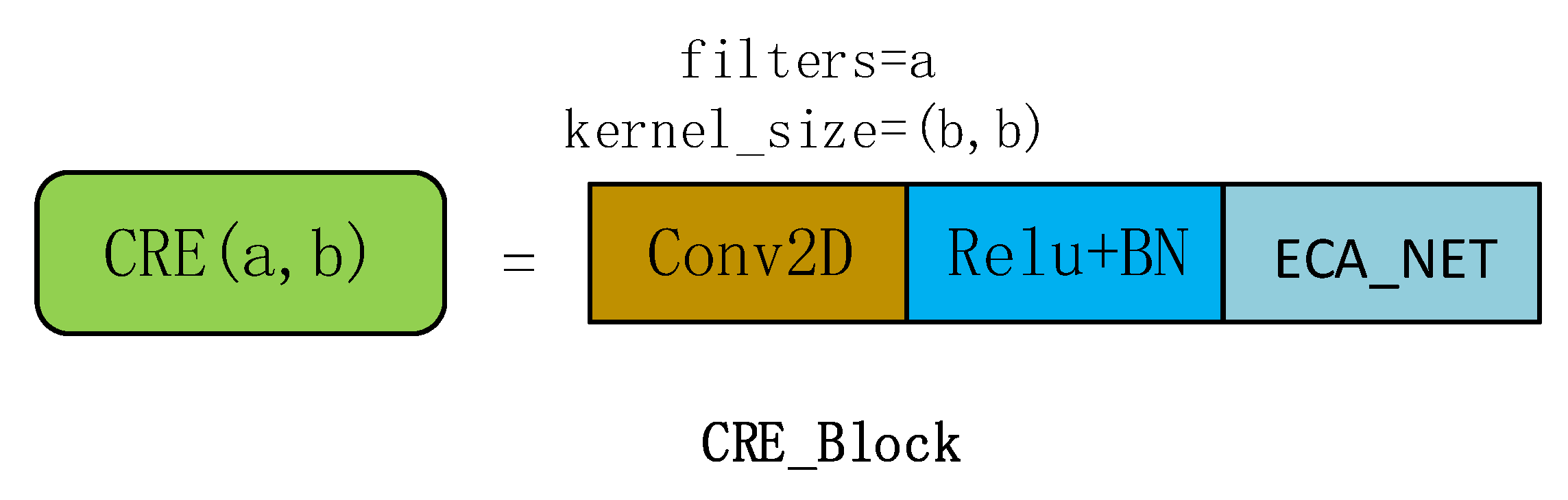
Considering that a deeper network may cause gradient dispersion, an improved residual structure was used to build a neural network model, i.e., the ECA residual net. This structure can retain weak image information, effectively deepen the neural network, extract high-level abstract feature information of the image without increasing the number of network parameters, and solve the problem of network degradation. This network structure is presented in Figure 3. Given an input feature of {c, c, d}, it undergoes a batch normalization (BN) operation, which greatly improves the processing speed of the subsequent data information. The output is then input to a two-dimensional convolutional layer utilizing a kernel of (3, 3) with a step size of a, and a ReLU activation function. The output then passes through a BN process. The latter convolutional BN process is repeated, and then, the output passes through an ECA-NET feature extraction module. The ECA-NET output result is added to the feature map that passed the BN layer for the first time, and ultimately the output is provided by a ReLU activation function. It is worth noting that the output result assigns lower weights to insensitive features in the hyperspectral domain and higher weights to abstract deep features.

2.4. CRE_Block

The CRE_Block comprises a two-dimensional convolution process, a ReLU activation function, a batch normalization, and an attention mechanism (ECA_NET) to aggregate the spatial spectrum characteristics of the image. The module structure is depicted in Figure 4.

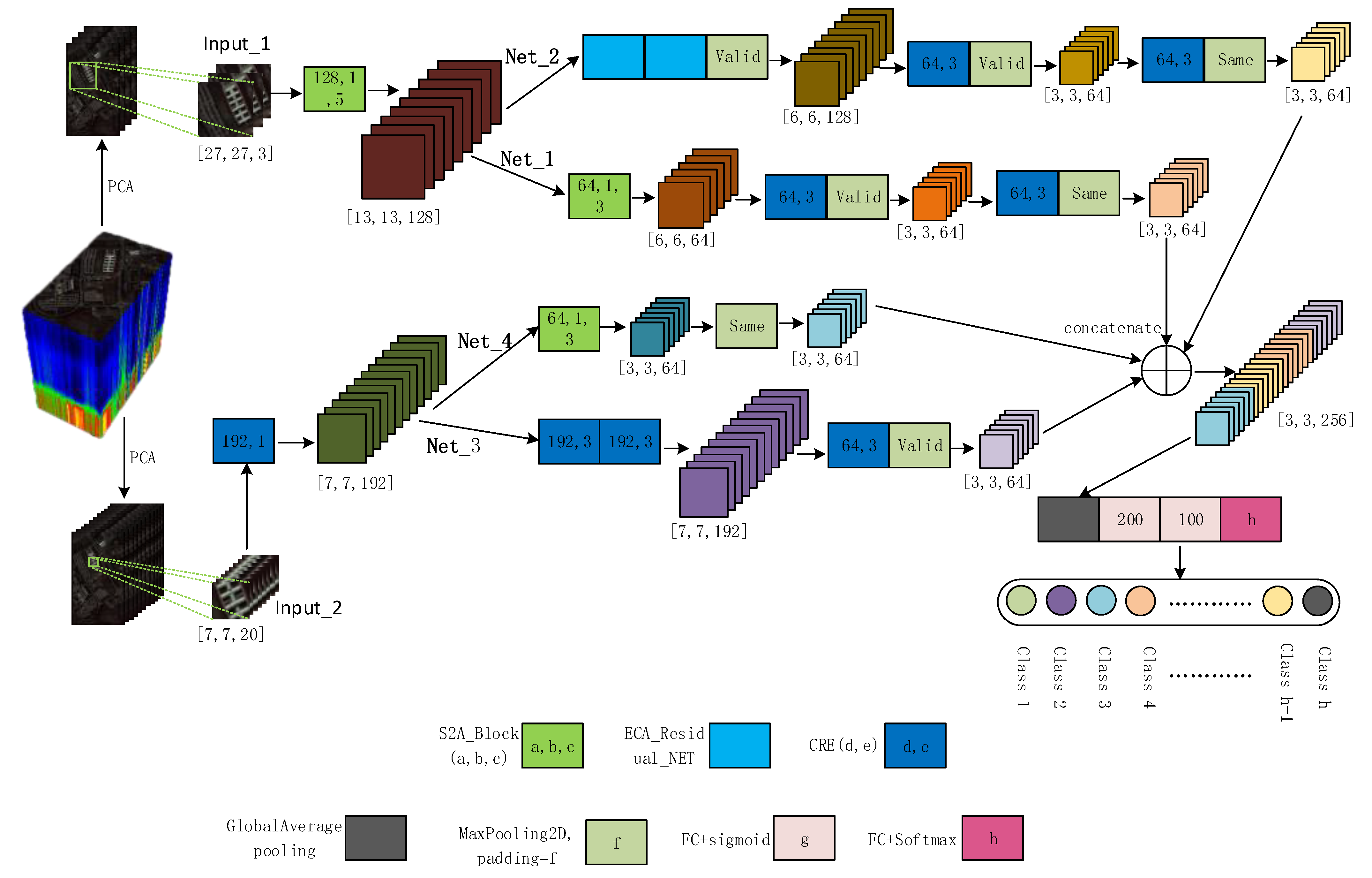
2.5. Overall Network Structure of the Suggested Deep Classification Technique

The proposed deep network architecture uses the PCA algorithm to separate and extract the image space–spectrum features for the first time, and then uses the S2A module, which contains the attention mechanism and the improved residual network structure, to extract the spatial and spectral features of the image multiple times. Additionally, in the middle of the model, we also exploit the ECA-NET network, and finally perform a feature fusion process to merge the features from the distinct subnetwork, e.g., S2A module, ECA-NET, etc., and input the fused feature to a fully connected layer for classification. The proposed model structure is shown in Figure 5.
We utilize the PCA method to reduce the image spectral dimensions to 3 and 20 and select patches of different sizes to create two inputs (Input_1, Input_2) with size {27,27,3} and {7,7,20}, respectively. The feature map with the large patch size and the small spectral dimension, i.e., Input_2, contains more spatial feature information, while the feature map with the small patch size but large spectral dimension contains more spectral feature information, i.e., Input_1.
Initially, we input to our architecture the Input_1 feature map and extract the space–spectrum feature information of the image through an S2A block module with 128 filters and convolution kernels of (1,1) and (5,5). The output tensor of the S2A block is {13, 13, 128}, which is then input to the subnetworks Net_1 and Net_2, respectively. The Net_1 network first consists of an S2A block module with 64 filters and convolution kernels of (1, 1), (3, 3), and comprises of two CRE modules followed by MaxPooling operations. Ultimately, the output shape is of this subnetwork is {3, 3, 64}. Regarding the Net_2 subnetwork, the Input_1 feature tensor is input to two ECA_Residual_NET modules and then passes through two CRE modules and MaxPooling operations to obtain an output feature map (map2) of size {3,3,64}. Considering the Input_2 feature map, it is initially input to the two CRE modules to create a feature map of {7, 7, 192} that is sent to Net_3 and Net_4, respectively. The Net_3 network contains two CRE modules with different parameters followed by a MaxPooling operation that outputs a feature map (map3) with shape {3, 3, 64}. The Net_4 network considers an S2A block module with 64 filters and (1, 1), (3, 3) convolution kernels followed by a MaxPooling layer, to ultimately create an output feature map (map4) with shape {3, 3, 64}. Finally, the four output feature maps (maps) are concatenated to realize the multi-scale feature extraction of the hyperspectral image, first through the global average pooling layer (GAP), and then through the two fully connected layers with two parameters (the variable g is used to represent the number of layers in the legend) respectively of 200, 100. The connection layer adds the sigmoid activation function, and finally, the hyperspectral image classification information is obtained through a fully connected layer (the variable h represents the classification type) plus the Softmax activation function output. This paper extracts hyperspectral image information from four different scales for many times, and finally connects the extracted features, which effectively improves the accuracy of the hyperspectral image classification problem.

3. Experimental Platform and Experimental Result

All experiments are performed on a Windows 10 system, with an Intel Core i7-9600 CPU, an Nvidia GeForce GTX2060S GPU with 8 GB video memory, using the TensorFlow2.3 deep learning framework and a Python 3.7 compiler. During trials, we challenge the classification performance of the proposed network model against current hyperspectral classification models on various datasets. Additionally, we also analyze the influence of various hyperparameters on the classification performance of our model. The evaluation metrics used are the overall accuracy (OA), the average classification (AA) accuracy, and the Kappa coefficient.

3.1. Introduction of the Dataset

3.1.1. Pavia University Dataset
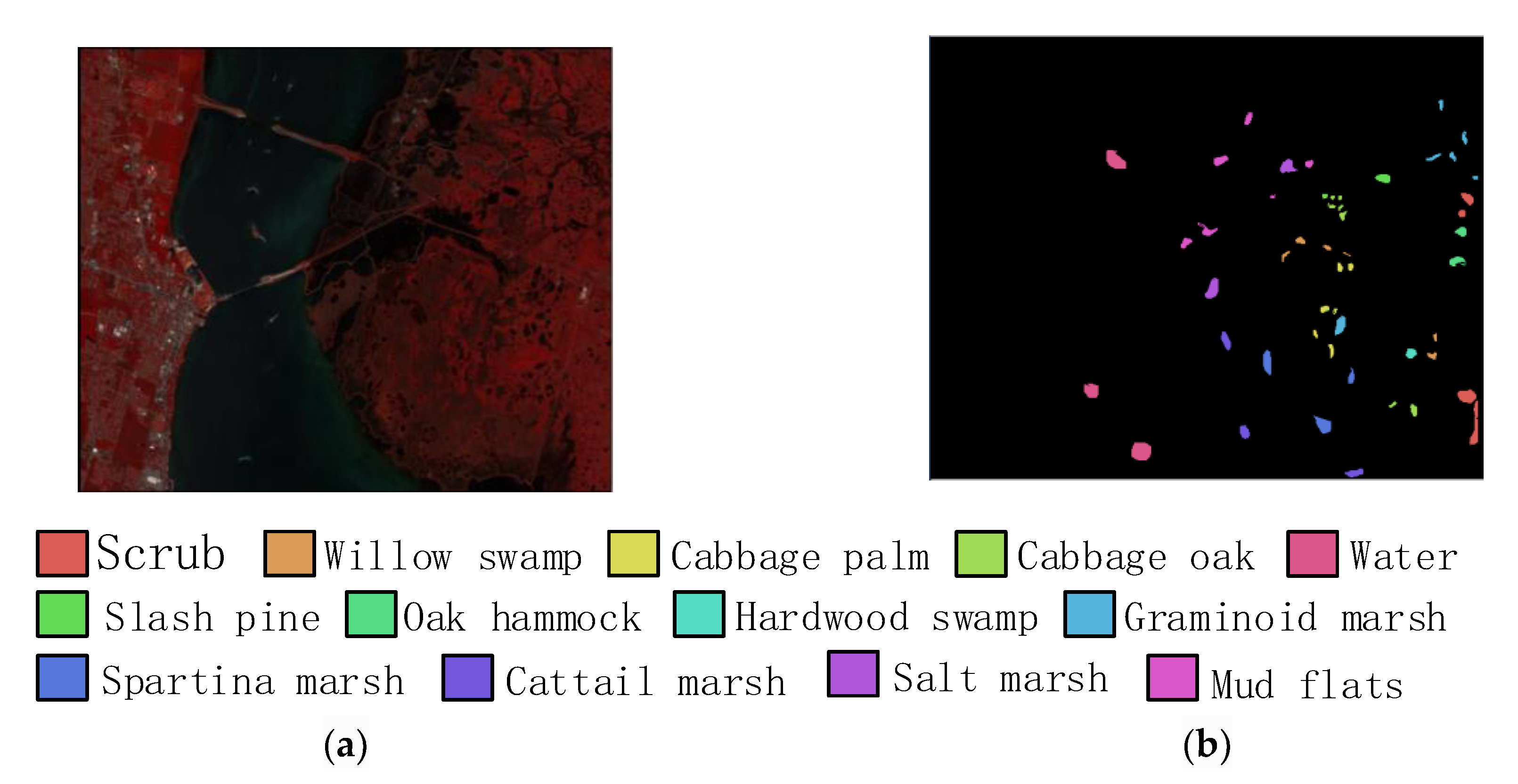
The Pavia University dataset (UP) is a collection of hyperspectral images obtained from Pavia, Italy, with an example presented in Figure 6a. The spatial image size is 610   ×   340 pixels, while the spectral information has 103 effective bands, and the wavelength range is 430~860 nm. The spatial resolution is 1.3 m, including nine types of ground features such as grass, asphalt, bricks, etc. The real ground feature map is shown in Figure 6b, with 42,776 pixels marked in total. During trials, as in work [20], we randomly select 10%, 10%, and 70% of the whole labeled samples as training, validation, and testing sets for the datasets. The dataset feature types, along with the training and test set sample information are shown in Table 1.

3.1.2. KSC Dataset

The KSC dataset is a hyperspectral imagery collection obtained from the Kennedy Space Center. An example is shown in Figure 7a. The spectral information has a total of 176 effective bands, the spatial image size is 614   ×   512 pixels, and the wavelength range is 400~2450 nm, including scrub, oak hammock, slash pine, and 13 other class categories. The ground truth feature map is shown in Figure 7b, where a total of 5211 pixels are labeled. During trials, as in work [20], we randomly select 20%, 10%, and 70% of the whole labeled samples as training, validation, and testing sets for the datasets. The dataset feature types, along with the training and test set sample quantity information are shown in Table 2.

3.1.3. Indian Pines Dataset

The Indian Pines dataset (IN) was collected in Indiana, USA. An example of that dataset is shown in Figure 8a. The spectral information has a total of 200 effective bands, the spatial image size is 145   ×   145 pixels, the wavelength range is 400~2500nm, and the spatial resolution is 20 m. This dataset includes 16 feature categories such as alfalfa, corn, oats, etc. The ground truth feature map is shown in Figure 8b, with 10,249 pixels labeled. Similarly, to the previous datasets, during our experiments, as in work [20], we randomly select 20%,10%, and 70% of the whole labeled samples as training, validation, and testing sets for the datasets. Table 3 shows the types of object classes in the dataset, the number of samples in the training set, and the test set.

3.2. Analysis of Experimental Results

During trials, we challenge our proposed deep network architecture against PCA [7], SVM [5], two-dimensional convolutional neural network (2D-CNN) [14], three-dimensional convolutional neural network (3D-CNN) [18], three-dimensional residual convolution structure (RES-3D-CNN) [36], and the space–spectrum joint deep network (SSRN) [20].

3.2.1. Parameter Setting

In this section, we analyze the interplay between the parameter setup and the classification performance of the proposed model. The tuned parameters include learning rate, batch_size, and training sample ratio. Regarding learning rate, it controls the speed of the gradient descent during the training process, with the appropriate learning rate parameters effectively controlling the convergence ability and speed of the model. We evaluate our network by using six learning rates with different sizes, i.e., 0.00005, 0.0001, 0.0003, 0.0005, 0.001, and 0.005. The test results are shown in Figure 9, from which we observe that when the learning rate is 0.0003, the classification performance on the three datasets is better. Additionally, tuning the learning rate parameter has less impact on the accuracy of the Pavia University dataset and a greater impact on the Indian Pines dataset.
The next trial investigates how the batch size affects the overall accuracy of our method. The batch size refers to the number of samples selected during training. Choosing a suitable batch_size can effectively improve the memory utilization and improve the convergence accuracy of the model. We challenge the performance on batch_size of 16, 32, 64, and 128, with the corresponding results presented in Figure 10. Our trials demonstrate that when the batch_size is 16, the classification attained on the three datasets is better. However, in the case of fewer training samples, a smaller batch_size will perform better.
Our final trial considers utilizing 5%, 10%, 20%, 30%, and 40% of the sample data as the training set. After our model being trained on the respective sample dataset, we test our network, with the corresponding results presented in Figure 11. From the latter figure, we conclude that as the training samples increase, the overall accuracy of our model is increasing. To compare with other networks, we adopt the strategy of [20], and we randomly select 20%, 10%, and 70% of the whole labeled samples as training, validation, and testing sets, respectively, for the Indian Pines and KSC datasets. For the Pavia University dataset, we employ a 10%, 10%, and 80% strategy.

3.2.2. Pavia University Dataset

Figure 12 shows the accuracy curve of each classification model in the Pavia University dataset. It can be seen that our deep network model converges quickly, and the classification accuracy is higher compared to the competitor techniques. The model is trained on the Pavia University dataset in just 3 minutes and 31 seconds. Table 4 shows the classification accuracy of each model for all nine object classes. From that table, we observe that our classification network manages 99.67% OA, 99.21% AA, and the Kappa coefficient is 0.9971. Compared to the competitor algorithms, our method attains higher classification results. Specifically, the OA of the PCA algorithm is 87.23%, the AA is 88.15%, and the Kappa coefficient is 0.85. Under the same conditions, the overall classification accuracy of the SVM algorithm compared to PCA is increased by 3.3%, and the average classification accuracy is increased by 2.1%, but still inferior to our method. The OA of 2D-CNN is 93.33%, AA is 94.17%, and the Kappa coefficient is 0.92, while the OA of the 3D-CNN is 94.68%, AA is 95.37%, and the Kappa coefficient is 0.94. Compared to the traditional algorithms, the classification accuracy of both CNN methods is greatly improved reflecting the superiority of deep learning in the hyperspectral classification problem. Compared with 3D-CNN, the overall classification accuracy of the 3D residual network is increased by 3.1%, and the average classification accuracy is increased by 2.8%. SSRN network presents an appealing classification performance attaining 98.17% OA, 98.64% AA, and a Kappa coefficient of 0.98. We bolded the data with the highest accuracy of feature classification. The experimental results show that the overall performance of our proposed network model is better than other models.
Figure 13 depicts some classification examples per method. It can be seen that the PCA and SVM classification algorithms have poor accuracy and present more misclassifications. The 2D-CNN classification results are slightly improved but still contain many misclassifications. The 3D-CNN, RES-3D, and SSRN models attain improved classification accuracy. However, the classification results of the suggested deep network architecture show an even more accurate classification, as they do not contain salt and pepper noise, and the boundaries are smooth and fit.

3.2.3. KSC Dataset

The accuracy curve of each classification model for the KSC dataset are presented in Figure 14. It can be seen that as the epoch increases, the classification accuracy rate is increasing. The model is trained on the KSC dataset in just 1 minute and 43 seconds. Table 5 shows the precise classification indicators of each method, where the proposed technique attains the highest metrics compared to the competitor methods, i.e., 99.81% OA, 99.74% AA, and 0.9952 Kappa metric. Additionally, from this table we observe that the overall accuracy of PCA, SVM, 2D-CNN, 3D-CNN, RES-3D, and SSRN has improved by 17.72%, 11.05%, 9.56%, 6.29%, 2.34%, and 1.65%, respectively, in the KSC dataset examined here compared to the Pavia University dataset evaluated in Section 3.2.2. Accordingly, the average accuracy has increased by 18.18%, 10.57%, 8.42%, 5.54%, 2.49%, 1.61%. This trial shows that RES-3D and the suggested network manage a better classification and highlights that our method is more suitable for a real landmark map. Classification examples per method are shown in Figure 15. Our network has started to converge in the 4th Epoch, and its performance is better than that of other models. Our network model shows better performance on the problem of hyperspectral image classification.

3.2.4. Indian Pines Dataset

Figure 16 shows the accuracy curve of each classification model in the Indian Pines dataset. Overall, the proposed deep classification network has the fastest convergence and the highest accuracy, and its classification performance is better compared to the competitor models. The model is trained on the Indian Pines dataset in just 1 minute and 37 seconds. Table 6 shows the precise classification index of each model for 13 classes of ground objects. From the latter table, we observe that the overall accuracy value of the proposed network is 24.05%, 18.81%, 13.22%, 5.09%, 1.79%, and 1.10% compared to PCA, SVM, 2D-CNN, 3D-CNN, RES-3D, and SSRN, respectively. Accordingly, the average accuracy attained by our model is higher by 24.02%, 18.02%, 14.22%, 5.48%, 2.09%, 1.17%, respectively, reaching a classification of 99.45% average accuracy and a Kappa coefficient of 0.9961. The classification results of each model are shown in Figure 17. It can be seen that the classification effect of PCA, SVM, and 2D-CNN models is poor, with more noise and speckles. 3D-CNN and RES-3D model classification results are less noisy, which improves the classification accuracy of these models. SSRN and the suggested network both attain an appealing classification accuracy. It can be seen from Table 6 that the classifier shows that the classification accuracy of Corn—min till is slightly lower, while the classification accuracy of the other classes is higher. In addition, it can be seen from Figure 16 that our network converges extremely fast and achieved good classification accuracy in the 6th Epoch, which is also due to other models.

4. Conclusions

This paper studies the application of deep learning for hyperspectral image classification. Aiming at the characteristics of a wide range of hyperspectral images, high spectral resolution, and a large amount of redundant information, a multi-scale residual convolution with ECA-NET is designed. The neural network model extracts image feature information. The model uses ECA-Net, improved residual network, and other structures to extract hyperspectral image information multiple times from different scales, can fully fuse and extract the space–spectrum characteristics of the image and effectively solve the problems of gradient dispersion and sample information redundancy. We challenge our suggested classification model against six current classification models, i.e., PCA, SVM, 2D-CNN,3D-CNN, RES-CNN, SSRN, on the Pavia University, KSC, and Indian Pines datasets, and demonstrate that our algorithm can effectively classify various object classes and has certain advantages in dealing with hyperspectral classification problems. Our proposed method successfully attains 99.82%, 99.81%, and 99.37% overall accuracy, respectively, on the three different free datasets. All trials demonstrate the superiority of our method against the competitor ones attaining a high classification accuracy. Future work shall focus on studying spatial and spectral feature fusion methods to enhance the feature extraction process, improve the network structure and parameters, accelerate the model convergence, and reduce network training time.

Author Contributions

Conceptualization, Y.Q. and W.L.; methodology, Y.Q.; software, Y.Q.; validation, Y.Q. and W.L.; formal analysis, Y.Q.; writing—original draft preparation, Y.Q. and W.L.; writing—review and editing, Y.Q.; visualization, W.L. All authors have read and agreed to the published version of the manuscript.

Funding

This research received no external funding.

Conflicts of Interest

The authors declare no conflict of interest.

References

  1. Bioucas-dias, J.M.; Plaza, A.; Camps-valls, G.; Scheunders, P.; Nasrabadi, N.; Chanussot, J. Hyperspectral Remote Sensing Data Analysis and Future Challenges. IEEE Geosci. Remote Sens. Mag. 2013, 1, 6–36. [Google Scholar] [CrossRef] [Green Version]
  2. Li, W.; Wu, G.; Zhang, F.; Du, Q. Hyperspectral image classification using deep pixel-pair features. IEEE Trans. Geosci. Remote Sens. 2016, 55, 844–853. [Google Scholar] [CrossRef]
  3. Hughes, G. On the mean accuracy of statistical pattern recognizers. IEEE Trans. Inf. Theory 1968, 14, 55–63. [Google Scholar] [CrossRef] [Green Version]
  4. Maghsoudi, Y.; Zoej, M.J.V.; Collins, M. Using class-based feature selection for the classification of hyperspectral data. Int. J. Remote Sens. 2011, 32, 4311–4326. [Google Scholar] [CrossRef]
  5. Melgani, F.; Bruzzone, L. Classification of hyperspectral remote sensing images with support vector machines. IEEE Trans. Geosci. Remote Sens. 2004, 42, 1778–1790. [Google Scholar] [CrossRef] [Green Version]
  6. Li, J.; Bioucas-Dias, J.; Plaza, A. Spectral–spatial hyperspectral image segmentation using subspace multinomial logistic regression and Markov random fields. IEEE Trans. Geosci. Remote Sens. 2012, 50, 809–823. [Google Scholar] [CrossRef]
  7. Licciardi, G.; Marpu, P.; Chanussot, J.; Benediktsson, J. Linear versus nonlinear PCA for the classification of hyperspectral data based on the extended morphological profiles. IEEE Geosci. Remote Sens. Lett. 2012, 9, 447–451. [Google Scholar] [CrossRef] [Green Version]
  8. Deng, Y.J.; Li, H.C.; Pan, L.; Shao, L.Y.; Du, Q.; Emery, W.J. Modified tensor locality preserving projection for dimensionality reduction of hyperspectral images. IEEE Geosci. Remote Sens. Lett. 2018, 15, 277–281. [Google Scholar] [CrossRef]
  9. Villa, A.; Benediktsson, J.A.; Chanussot, J.; Jutten, C. Hyperspectral Image Classification With Independent Component Discriminant Analysis. IEEE Trans. Geosci. Remote Sens. 2011, 49, 4865–4876. [Google Scholar] [CrossRef] [Green Version]
  10. Liu, J.; Wu, Z.; Wei, Z.; Xiao, L.; Sun, L. Spatial-spectral kernel sparse representation for hyperspectral image classification. IEEE J. Sel. Top. Appl. Earth Obs. Remote Sens. 2013, 6, 2462–2471. [Google Scholar] [CrossRef]
  11. Gao, L.; Hong, D.; Yao, J.; Zhang, B.; Gamba, P.; Chanussot, J. Spectral Superresolution of Multispectral Imagery with Joint Sparse and Low-Rank Learning. IEEE Trans. Geosci. Remote Sens. 2020, 1–12. [Google Scholar] [CrossRef]
  12. Chen, Y.; Lin, Z.; Zhao, X.; Wang, G.; Gu, Y. Deep learning-based classification of hyperspectral data. IEEE J. Sel. Top. Appl. Earth Obs. Remote Sens. 2014, 7, 2094–2107. [Google Scholar] [CrossRef]
  13. Hu, W.; Huang, Y.Y.; Wei, L.; Zhang, F.; Li, H.C. Deep Convolutional Neural Networks for Hyperspectral Image Classification. J. Sens. 2015, 2015, 1–12. [Google Scholar] [CrossRef] [Green Version]
  14. Hao, S.; Wang, W.; Ye, Y.; Nie, T.; Bruzzone, L. Two-stream deep architecture for hyperspectral image classification. IEEE Trans. Geosci. Remote Sens. 2017, 56, 2349–2361. [Google Scholar] [CrossRef]
  15. Mei, S.; Ji, J.; Bi, Q.; Hou, J.; Du, Q.; Li, W. Integrating spectral and spatial information into deep convolutional neural networks for hyperspectral classification. In Proceedings of the IEEE International Geoscience and Remote Sensing Symposium (IGARSS), Beijing, China, 10–15 July 2016; pp. 5067–5070. [Google Scholar]
  16. Chen, C.; Zhang, J.; Zheng, C.; Yan, Q.; Xun, L. Classification of hyperspectral data using a multi-channel convolutional neural network. In Proceedings of the 14th International Conference on Intelligent Computing (ICIC), Wuhan, China, 15–18 August 2018; pp. 81–92. [Google Scholar]
  17. Gao, F.; Huang, T.; Sun, J.; Wang, J.; Hussain, A.; Yang, E. A New Algorithm of SAR Image Target Recognition Based on Improved Deep Convolutional Neural Network. Cogn. Comput. 2019, 11, 809–824. [Google Scholar] [CrossRef] [Green Version]
  18. Rao, M.; Tang, P.; Zhang, Z. A Developed Siamese CNN with 3D Adaptive Spatial-Spectral Pyramid Pooling for Hyperspectral Image Classification. Remote Sens. 2020, 12, 1964. [Google Scholar] [CrossRef]
  19. Lee, H.; Kwon, H. Going deeper with contextual CNN for hyperspectral image classification. IEEE Trans. Image Process. 2017, 26, 4843–4855. [Google Scholar] [CrossRef] [Green Version]
  20. Zhong, Z.; Li, J.; Luo, Z.; Chapman, M. Spectral-spatial residual network for hyperspectral image classification: A 3-D deep learning framework. IEEE Trans. Geosci. Remote Sens. 2018, 56, 847–858. [Google Scholar] [CrossRef]
  21. Wu, P.; Cui, Z.; Gan, Z.; Liu, F. Residual Group Channel and Space Attention Network for Hyperspectral Image Classification. Remote Sens. 2020, 12, 2035. [Google Scholar] [CrossRef]
  22. Mou, L.; Zhu, X.X. Learning to Pay Attention on Spectral Domain: A Spectral Attention Module-Based Convolutional Network for Hyperspectral Image Classification. IEEE Trans. Geosci. Remote Sens. 2019, 58, 110–122. [Google Scholar] [CrossRef]
  23. Wang, L.; Peng, J.T.; Sun, W.W. Spatial–Spectral Squeeze-and-Excitation Residual Network for Hyperspectral Image Classification. Remote Sens. 2019, 11, 884. [Google Scholar] [CrossRef] [Green Version]
  24. Zhong, Z.; Li, J.; Clausi, D.A.; Wong, A. Generative Adversarial Networks and Conditional Random Fields for Hyperspectral Image Classification. IEEE Trans. Cybern. 2020, 50, 3318–3329. [Google Scholar] [CrossRef] [PubMed] [Green Version]
  25. Yuan, Y.; Zheng, X.T.; Lu, X.Q. Hyperspectral image superresolution by transfer learning. IEEE J. Sel. Top. Appl. Earth Obs. Remote Sens. 2017, 10, 1963–1974. [Google Scholar] [CrossRef]
  26. Roy, S.K.; Krishna, G.; Dubey, S.R.; Chaudhuri, B.B. HybridSN: Exploring 3-D-2-D CNN Feature Hierarchy for Hyperspectral Image Classification. IEEE Geosci. Remote Sens. Lett. 2020, 17, 277–281. [Google Scholar] [CrossRef] [Green Version]
  27. Niu, R. HMANet: Hybrid Multiple Attention Network for Semantic Segmentation in Aerial Images. arXiv 2020, arXiv:2001.02870. [Google Scholar]
  28. Zhang, M.; Li, W.; Du, Q. Diverse region-based CNN for hyperspectral image classification. IEEE Trans. Image Process. 2018, 27, 2623–2634. [Google Scholar] [CrossRef] [PubMed]
  29. Fang, L.Y.; LI, S.T.; Kang, X.D.; Jon, A. Spectral spatial classification of hyperspectral images with a superpixel-based discriminative sparse model. IEEE Trans. Geosci. Remote Sens. 2015, 53, 4186–4201. [Google Scholar] [CrossRef]
  30. Wang, Q.L.; Wu, B.G.; Zhu, P.F.; Li, P.H.; Zuo, W.M.; Hu, Q.H. ECA-Net: Efficient Channel Attention for Deep Convolutional Neural Networks. In Proceedings of the IEEE/CVF Conference on Computer Vision and Pattern Recognition (CVPR), Seattle, WA, USA, 13–19 June 2020; pp. 11531–11539. [Google Scholar]
  31. Hu, J.; Shen, L.; Albanie, S.; Sun, G.; Wu, E.H. Squeeze-and-Excitation Networks. arXiv 2018, arXiv:1709.01507v4. [Google Scholar]
  32. Lin, M.; Chen, Q.; Yan, S. Network in network. arXiv 2013, arXiv:1312.4400. [Google Scholar]
  33. Li, L.; Yin, J.H.; Jia, X.P.; Li, S.; Han, B.N. Joint Spatial-Spectral Attention Network for Hyperspectral Image Classification. IEEE Geosci. Remote Sens. Lett. 2020, 130, 38–45. [Google Scholar] [CrossRef]
  34. Ioffe, S.; Szegedy, C. Batch normalization: Accelerating deep network training by reducing internal covariate shift. In Proceedings of the 32nd International Conference on International Conference on Machine Learning, Paris, France, 6–11 July 2015; pp. 448–456. [Google Scholar]
  35. Nair, V.; Hinton, G.E. Rectified linear units improve restricted Boltzmann machines. In Proceedings of the 27th International Conference on International Conference on Machine Learning (ICML), Haifa, Israel, 21–24 June 2010; Omnipress: Madison, WI, USA, 2010; pp. 807–814. [Google Scholar]
  36. Liu, B.; Yu, X.; Zhang, P.; Tan, X. Deep 3D convolutional network combined with spatial-spectral features for hyperspectral image classification. Acta Geod. Cartogr. Sin. 2019, 48, 53–63. [Google Scholar]
Figure 1. Efficient channel attention network (ECA-NET) block.
Remotesensing 13 00335 g001
Figure 2. S2A block.
Remotesensing 13 00335 g002
Figure 3. ECA residual net.
Remotesensing 13 00335 g003
Figure 4. CRE block.
Remotesensing 13 00335 g004
Figure 5. Overall network structure.
Remotesensing 13 00335 g005
Figure 6. Pavia University dataset, (a) original image, (b) mark map of real ground objects.
Remotesensing 13 00335 g006
Figure 7. KSC dataset, (a) original image, (b) mark map of real ground objects.
Remotesensing 13 00335 g007
Figure 8. Indian Pines dataset, (a) original image, (b) mark map of real ground objects.
Remotesensing 13 00335 g008
Figure 9. Overall accuracy (OA, %) of the proposed network with different learning rates in Indian Pines (IN), Pavia University (UP), and KSC dataset.
Remotesensing 13 00335 g009
Figure 10. OA (%) of the proposed network with different batch_size in IN, UP, and KSC dataset.
Remotesensing 13 00335 g010
Figure 11. OA (%) of the proposed network with different training samples in IN, UP, and KSC dataset.
Remotesensing 13 00335 g011
Figure 12. Overall accuracy curve of different models in Pavia University dataset.
Remotesensing 13 00335 g012
Figure 13. (ag) Classification map of principal components analysis (PCA), support vector machine (SVM), 2D convolutional neural network (CNN), 3D-CNN, RES-3D, space–spectrum joint deep network (SSRN), and proposed on Pavia University dataset.
Remotesensing 13 00335 g013
Figure 14. Overall accuracy curve of different models in KSC dataset.
Remotesensing 13 00335 g014
Figure 15. (ag) Classification map of PCA, SVM, 2D-CNN, 3D-CNN, RES-3D, SSRN, and proposed on KSC dataset.
Remotesensing 13 00335 g015
Figure 16. Overall accuracy curve of different models in Indian Pines dataset.
Remotesensing 13 00335 g016
Figure 17. (ag) Classification map of PCA, SVM, 2D-CNN, 3D-CNN, RES-3D, SSRN, and proposed on Indian Pines dataset.
Remotesensing 13 00335 g017aRemotesensing 13 00335 g017b
Table 1. Training validation and testing sample numbers for the Pavia University dataset.
NumberClassTrainingValidationTestTotal Samples
1Asphalt66366353056631
2Meadows1864186414,92118,649
3Gravel20920916812099
4Trees30630624523064
5Sheets13413410771345
6Bare Soil50250240255029
7Bitumen13313310641330
8Bricks36836829463682
9Shadows9494759947
Total 4273427334,23042,776
Table 2. Training validation and testing sample numbers in KSC.
NumberClassTrainingValidationTest Total Samples
1Scrub15276533761
2Willow swamp4824171243
3Cabbage palm5025181256
4Cabbage oak5025177252
5Slash pine3216113161
6Oak hammock4623160229
7Hardwood swamp201075105
8Graminoid marsh8643302431
9Spartina marsh10452364520
10Cattail marsh8040284404
11Salt marsh8442293419
12Mud flats10050353503
13Water18693648927
Total 103851936545211
Table 3. Training validation and testing sample numbers in Indian Pines.
NumberClassTraining ValidationTest Total Samples
1Alfalfa843446
2Corn—no till28414210021428
3Corn—min till16683581830
4Corn4623168237
5Grass/pasture14673511730
6Grass/tress9648339483
7Grass/pasture—mowed 6 31928
8Hay—windrowed 94 47337478
9Soybeans—no till 194 97681972
10Soybeans—min till 490 24517202455
11Soybeans—clean till 118 59416593
12Wheat 40 20145205
13Woods 252 1268871265
14Buildings–grass–trees 76 38272386
15Stone–steel towers 18 96693
16Oats 4 21420
Total 20381019719210,249
Table 4. Classification results of different models in Pavia University.
ClassPCASVM2D-CNN3D-CNNRES-3DSSRNMy_Net
Asphalt76.6585.5793.800.97.1596.1898.8498.74
Meadows88.8686.5689.4393.4398.1097.23100.00
Gravel92.2489.4392.2794.4897.2199.8299.56
Trees90.3892.1794.1392.3995.3198.15100.00
Metal87.5685.6890.5194.3799.6499.4398.83
Soil85.5294.7992.3496.6897.7296.17100.00
Bitumen88.6790.6594.7293.4896.3196.5699.32
Bricks91.7392.4395.7897.7698.48100.00100.00
Shadows89.8692.7991.5694.34100.0098.3499.67
OA (%)87.2390.5393.3394.6897.7898.1799.82
AA (%)88.1590.2594.1795.3798.1798.6499.59
Kappa×10085.2389.2492.4894.4697.2598.7699.71
Table 5. Classification results of different models in KSC.
ClassPCASVM2D-CNN3D-CNNRES-3DSSRNMy_Net
Scrub66.7590.2884.4297.1997.9698.4699.37
Willow swamp93.5181.9679.6182.3896.2796.1799.82
Cabbage palm74.4375.6589.3494.2494.1798.4299.86
Cabbage oak92.3881.3594.9190.1896.7699.49100.00
Slash pine83.6392.8366.4870.6498.3296.3499.58
Oak hammock69.4374.5173.3470.3794.51100.00100.00
Hardwood swamp77.2879.6269.6474.1599.3499.37100.00
Graminoid marsh76.7295.8381.7290.4698.9499.8299.57
Spartina marsh82.7991.9290.1695.3797.8597.71100.00
Cattail marsh81.5688.1491.8798.48100.0099.42100.00
Salt marsh73.9291.4293.1699.1698.4299.45100.00
Mud flats69.3484.4888.6498.49100.0097.1899.75
Water85.1686.9495.54100.00100.00100.00100.00
OA (%)82.0988.7690.2593.5297.4798.1699.81
AA (%)81.5689.1791.3294.2097.2598.1399.74
Kappa×10081.7288.5691.9294.7797.2598.6499.52
Table 6. Classification results of different models in Indian Pines.
ClassPCASVM2D-CNN3D-CNNRES-3DSSRNMy_Net
Alfalfa72.4678.5374.3791.6297.3897.48100.00
Corn—no till69.3582.6186.6189.3395.37100.00100.00
Corn—min till71.5874.8491.4993.9798.6499.4699.25
Corn81.6279.7190.8295.9497.9296.56100.00
Grass—pasture67.3472.6773.5882.3497.9797.76100.00
Grass—tress81.2985.4282.6596.7299.4899.4898.56
Grass—pasture75.5281.1979.3781.6195.19100.00100.00
Hay—windrowed77.4383.5187.5179.3799.4199.56100.00
Oats86.9683.3790.4393.1997.7699.12100.00
Soybeans—no till80.8488.2893.1697.6498.84100.0099.17
Soybeans—min till82.6174.7695.1993.2897.1999.14100.00
Soybeans—clean till76.3986.5194.7298.76100.0098.08100.00
Wheat85.6482.4392.4999.2496.1597.58100.00
Woods77.5275.9790.8494.4998.76100.0099.38
Buildings–grass–trees84.4888.9187.3789.1996.1499.6798.89
Stone–steel towers73.4771.5886.6494.6499.3998.8499.38
OA (%)75.3280.5686.1594.2897.5898.2799.37
AA (%)75.4381.4385.2393.9797.3698.2899.45
Kappa×10075.8780.2685.6494.1597.4498.5299.61
Publisher’s Note: MDPI stays neutral with regard to jurisdictional claims in published maps and institutional affiliations.

