Evaluations of the Climatologies of Three Latest Cloud Satellite Products Based on Passive Sensors (ISCCP-H, Two CERES) against the CALIPSO-GOCCP

Abstract

In this study, the climatologies of three different satellite cloud products, all based on passive sensors (CERES Edition 4.1 [EBAF4.1 and SYN4.1] and ISCCP–H), were evaluated against the CALIPSO-GOCCP (GOCCP) data, which are based on active sensors and, hence, were treated as the reference. Based on monthly averaged data (ocean + land), the passive sensors underestimated the total cloud cover (TCC) at lower (TCC < 50%), but, overall, they correlated well with the GOCCP data (r = 0.97). Over land, the passive sensors underestimated the TCC, with a mean difference (MD) of −2.6%, followed by the EBAF4.1 and ISCCP-H data with a MD of −2.0%. Over the ocean, the CERES-based products overestimated the TCC, but the SYN4.1 agreed better with the GOCCP data. The ISCCP-H data on average underestimated the TCC both over oceanic and continental regions. The annual mean TCC distribution over the globe revealed that the passive sensors generally underestimated the TCC over continental dry regions in northern Africa and southeastern South America as compared to the GOCCP, particularly over the summer hemisphere. The CERES datasets overestimated the TCC over the Pacific Islands between the Indian and eastern Pacific Oceans, particularly during the winter hemisphere. The ISCCP-H data also underestimated the TCC, particularly over the southern hemisphere near 60° S where the other datasets showed a significantly enhanced TCC. The ISCCP data also showed less TCC when compared against the GOCCP data over the tropical regions, particularly over the southern Pacific and Atlantic Oceans near the equator and also over the polar regions where the satellite retrieval using the passive sensors was generally much more challenging. The calculated global mean root meant square deviation value for the ISCCP-H data was 6%, a factor of 2 higher than the CERES datasets. Based on these results, overall, the EBAF4.1 agreed better with the GOCCP data.

1. Introduction

Clouds cover a large portion of the Earth’s atmosphere at any given time and play a significant role in the weather and climate systems of the Earth by regulating its radiative balance and hydrological cycle. Based on numerous International Plan on Climate Change (IPCC) reports and modeling studies [1,2,3], the current general circulation models (GCMs) suffer from significant uncertainties in predicting the future climate. One of the main sources of these uncertainties is believed to be related to the representation of clouds [3,4,5,6,7]. As the temperature increases because of global warming, GCMs predict that the cloud cover will change because of radiative feedback mechanisms [8]. According to most GCMs, this feedback is positive as a result of rising high level cloud (HLC) and decreasing tropical low level clouds (LLC) [7,8]. The proper understanding of the change in distribution of clouds and cloud types is necessary for an accurate representation of clouds in the current GCMs and numerical weather prediction (NWP) models for improving the weather and climate predictions. However, these problems are not adequately addressed using observation data, largely because of a lack of reliable long-term, global-scale observation datasets. Satellite observations are increasingly being used for climate studies and evaluation of GCMs and NWP models because of the continuous near-global coverage that they provide. However, there are some uncertainties in satellite-based remote sensing of cloud cover because of the necessity to make certain approximations in the retrieval algorithms being used as well as other factors, including limitations in the type of sensors used for measuring the necessary parameters.

There are currently a number of satellite products based on both active and passive sensors. The products based on passive sensors include the Clouds and the Earth’s Radiant Energy System (CERES)-based products that largely use the Moderate Resolution Imaging Spectroradiometer (MODIS) sensor deployed on Aqua and Terra polar orbiting satellites and the International Satellite Cloud Climatology Project (ISCCP) data that use retrievals from multiple satellite platforms. The passive sensors retrieve clouds by sensing the reflected sunlight or emission of radiation from clouds and surfaces. As a result, they have some limitations since retrieval of cloud properties is difficult over bright and cold surfaces, such as near polar regions, and no visible retrievals can be made during the night. The ISCCP dataset has the longest record, starting from 1983, but attempts at using the data to study the climate trend in cloud cover have been questioned [9]. However, later the data were used after some empirical corrections [10]. On the other hand, the active sensors such as the Cloud-Aerosol Lidar and Infrared Pathfinder Satellite Observation (CALIPSO) data have fewer limitations and, hence, can provide more accurate measurement of clouds and are more appropriate for climate studies as well as providing a reference for the data collected using the passive sensors [11,12,13,14]. The active sensors are particularly useful for retrieving optically thin cirrus clouds that lead to capturing more high-level clouds, close to 20% to 30% as compared to the cloud products that are based on passive sensors such as the ISCCP and MODIS [14]. However, the CALIPSO-based cloud products that employ different retrieval algorithms also give different results [15,16], indicating some uncertainties. However, regardless of the algorithm used, the CALIPSO-based data generally capture more optically thin clouds as compared to the passive sensors [14]. There are no comprehensive comparisons of the CALIPSO data against ground-based measurements on a global scale, partly because ground-based observations are so sparse, particularly over the oceans. There are, however, some examples of localized studies that compared the CALIPSO and some other datasets based on passive satellite sensors against ground based measurements [17,18], and the results showed that the active sensors provide better results as compared to the passive sensors. The authors of [17] compared TCC based on the GCM-Oriented CALIPSO Cloud Product (CALIPSO-GOCCP) and ground-based observations using radar and lidar at Summit, Greenland. According to [17], the GOCCP data generally agreed with the ground-based observation better than the other passive satellite sensors, particularly in liquid phase clouds. On average, CALIPSO-GOCCP reported the TCC by about 6.7% as compared to the passive sensors. The authors of [18] compared the ISCCP-H data against surface-based measurement using the European Climate Assessment and Dataset (ECA&D) over Europe and found that the ISCCP-H overestimated the TCC by 5.2%. As is shown below, this is consistent with the finding in this study. These satellite products are also increasingly being updated, but there are very limited studies that are aimed at the evaluation of these products in literature.

The main purpose of this study was to evaluate the climatologies of TCC retrieved using passive sensors with updated algorithms provided by the CERES and ISCCP against the CALIPSO-GOCCP. The CALIPSO-GOCCP was chosen because it is increasingly being used for evaluation of GCMs and other satellite products, as discussed earlier, and also it is fully compatible with the GCM-lidar simulator data produced using the Cloud Feedback Model Intercomparison Project (CFMIP) Observation Simulator Package (COSP). The remainder of the paper is organized as follows. In Section 2, the materials and methods are described. In Section 3, the annual and seasonal climatologies of four satellite products are discussed. The summary and conclusions are given in Section 4

2. Materials and Methods

The datasets used in this study are given in

Table 1. The satellite cloud products used in this.

	Edition	Time Period	Frequency	Resolution	Sources
CERES -SYN1DEG	4.1	2000–2019	monthly	1° × 1°	CERES (NASA)
CERES-EBAF	4.1	2000–2019	monthly	1° × 1°	CERES (NASA)
ISCCP	H	2000–2017	monthly	1° × 1°	NOAA
CALIPSO-GOCCP		2007–2019	monthly	2° × 2°	CLIMSERV

. All the datasets were remapped to a common grid of the CALIPSO-GOCCP data using a first-order conservative remapping technique [19]. The brief descriptions of the datasets used in this study are given below.

2.1. Descriptions of the Datasets

2.1.1. ISCCP-H

The ISCCP satellite products include several cloud microphysical and meteorological parameters including TCC and type, cloud top temperature, cloud top pressure, and cloud optical thickness. The algorithms used to produce these products are described in several papers [20,21]. The ISCCP-H cloud properties were produced by using an algorithm [22,23] that was largely similar to the previous version (ISCCP-D) [20] that involved measured radiances at near visible (0.65 µm) and infrared (IR) (10.5 µm) wavelengths using the geostationary satellites within the 55°S and 55°N latitudes and the polar-orbiting satellites poleward of these regions. The cloud detection was performed using two basic steps [23]. First, it determined the radiances of the cloud-free regions using the data measured using both the IR and visible channels. Second, the cloudy regions were identified based on deviations from the cloud-free radiance values. By assuming that the presence of clouds increases and decrease the visible and IR radiances, respectively, thresholds were defined to identify cloudy pixels at 10-km spatial resolution [23] for various surface conditions [20,23]. The cloud amount was defined as the fraction of cloudy pixels to the total number of pixels determined within a 1° × 1° grid. This version of the ISCCP products uses input data from full-resolution Advanced Very-High-Resolution Radiometer (AVHRR) Global Area Coverage and higher-resolution geostationary data that can potentially improve the retrievals as compared to the earlier versions. In this study, the ISCCP-H dataset described in Table 1 was used.

2.1.2. CAPLISO-GOCCP

These are observation-based cloud products geared towards validating GCM simulated datasets and, hence, normally referred to as GCM-Oriented Cloud CALIPSO Product (GOCCP) [24]. The data are fully compatible with GCM-lidar simulator data produced using the Cloud Feedback Model Intercomparison Project (CFMIP) Observation Simulator Package (COSP) [25,26]. These data sets are derived from CALIPSO products and fully consistent with the ones simulated by the ensemble GCM + lidar simulator [24]. Based on [26], the cloud cover data were processed using a Cloud-Aerosol Lidar with Orthogonal Polarization following the identical steps as would be followed in a lidar simulator aimed at diagnosing the model cloud cover that CALIPSO would see from space. The steps taken for determining the cloud cover started with by analyzing the observed lidar backscattered ratio (SR) of total attenuated backscattered (ATB) signal to gas molecular ATB without consideration of aerosols at high horizontal resolution of 330 m by keeping the vertical resolution similar to the current GCMs. The cloudy pixels were identified based on SR values. The SR values SR > 5, 0.01 > SR < 1.2 and 1.2 < SR < 5 were flagged as cloudy, clear, or unclassified, respectively [24,27]. The cloud cover at a given level was defined as the number of cloudy pixels divided by the total number of pixels by ignoring the pixels that were associated with the total attenuation of the lidar backscattered signals (SR < 0.01). The cloud phases were identified based on the relationship between ATB and cross-polarized ATB (ATB┴) [24]. Based on this relationship, the cloud cover was classified as liquid, ice, or unidentified. These undefined clouds are normally found below other highly reflective clouds (SR > 30) or clouds having horizontally oriented ice crystals [27]. Studies show that supercooled mixed phase clouds are characterized by highly reflective layers in lidar imagery and a low depolarization ratio [28]; thus, most of these undefined cloud layers may be related to mixed phase clouds.

2.1.3. CERES Cloud Products

The TCC data used in this study included cloud products provided as part of the CERES EBAF (Energy Balanced and Field) and SYN1deg (Synoptic 1 degree) Edition 4.1 (EBAF4.1 and SYN4.1, respectively, from here on). The monthly mean cloud area fraction in EBAF4.1 was retrieved based on measurements taken using the MODIS instruments deployed on board the Terra and Aqua satellites flown at sun-synchronous orbit. The detailed description of this product is given in data-quality summary [29]. From March 2000 to June 2002, the data collected by the Terra satellite and from July onwards the average of both Terra and Aqua satellite data were used. The cloud cover retrieval process started with deriving the cloud properties based on a single satellite footprint Edition 4 (SSF4) [30], instantaneous data that uses an improved algorithm, as described in [31]. The instantaneous cloud cover determined based on SSF4 was spatially averaged at a 1° × 1° region and then linearly interpolated hourly to estimate the cloud cover between the MODIS observation points. The hourly regional cloud covers were then averaged over the month. Cloud properties for March 2000 through February 2016 were identical to those in EBAF Ed4.0. For March 2016 onwards, cloud properties were determined using MODIS Collection 6.1 (C6.1) radiances. This is because, after a slow degradation of two MODIS channels of Terra (6.7 μm and 8.6 μm) that got worse in March 2016, the MODIS team released C6.1 data products that corrected this problem onwards of March 2016.

In the SYN4.1 version of the cloud product, the cloud area fraction is based on both the CERES MODIS and multiple geostationary satellite (GEO) measurements [32]. Since the CERES MODIS data have limited time resolution, the addition of the hourly Geo data allowed the interpolation of the TCC covering the full diurnal cycle [32]. This version of the CERES data is primarily designed to have a high temporal resolution. As a result, the globally gridded (at 1° × 1° resolution) TCC data are available on the bases of monthly, monthly hourly, daily, 3-hourly, and hourly averages. In this study, only the monthly averaged version of the data was used.

3. Results

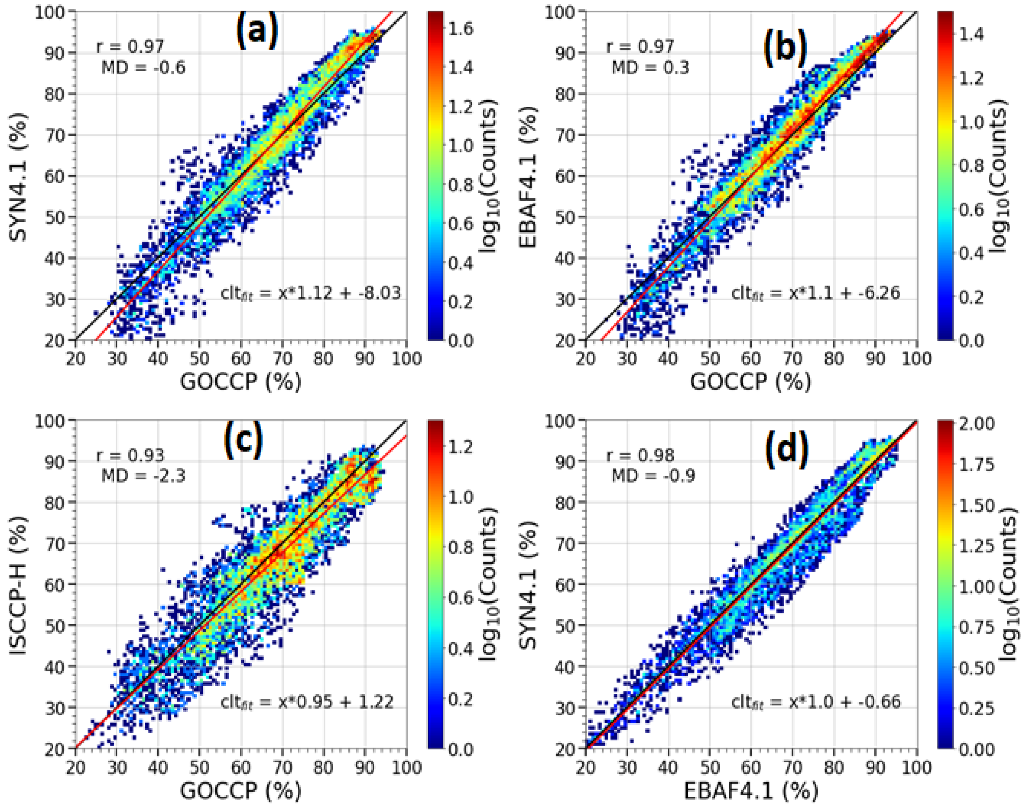
3.1. Comparisons over the Entire Globe (Ocean + Land): 2D Density Plots

Figure 1 shows 2D density plots of the annually averaged TCC obtained based on EBAF4.1 (a), SYN4.1 (b), and ISCCP-H (c), and determined based on the GOCCP data. The two CERES products EBAF4.1 and SYN4.1 were also compared in the plot (d). As revealed in the plots, the correlation coefficient between the GOCCP and CERES data sets (EBAF4.1 and SYN4.1) was close to 0.97, but the CERES (SYN4.1 and EBAF4.1) on average underestimated and overestimated by 0.6% and 0.3%, respectively. When the GOCCP data were compared against the ISCCP-H data, the correlation coefficient was slightly diminished to 0.93 and underestimated the TCC by a relatively higher value of −2.3%. Most of the discrepancies between the GOCCP and CERES datasets occurred at lower cloud covers (TCC < 50%) where the CERES datasets significantly underestimated the TCC ((a) and (b)). At higher cloud cover values, the agreement was improved but slightly overestimated the TCC at higher cloud covers (TCC > 70%). The underestimation of TCC at lower TCC was expected since the active sensors such as lidar used in CALIPSO captured more optically thin clouds as compared to the passive sensors normally used for collecting the CERES data sets. The comparisons of the ISCCP-H and GOCCP data also showed larger data spread and most of the data were below the 1:1 line as compared to the CERES products (c). As indicated in the plot (d), the two CERES products, EBAF4.1 and SYN4.1, showed excellent agreement with each other, with a correlation coefficient of 0.98. The best fit lines are also shown in the figure.

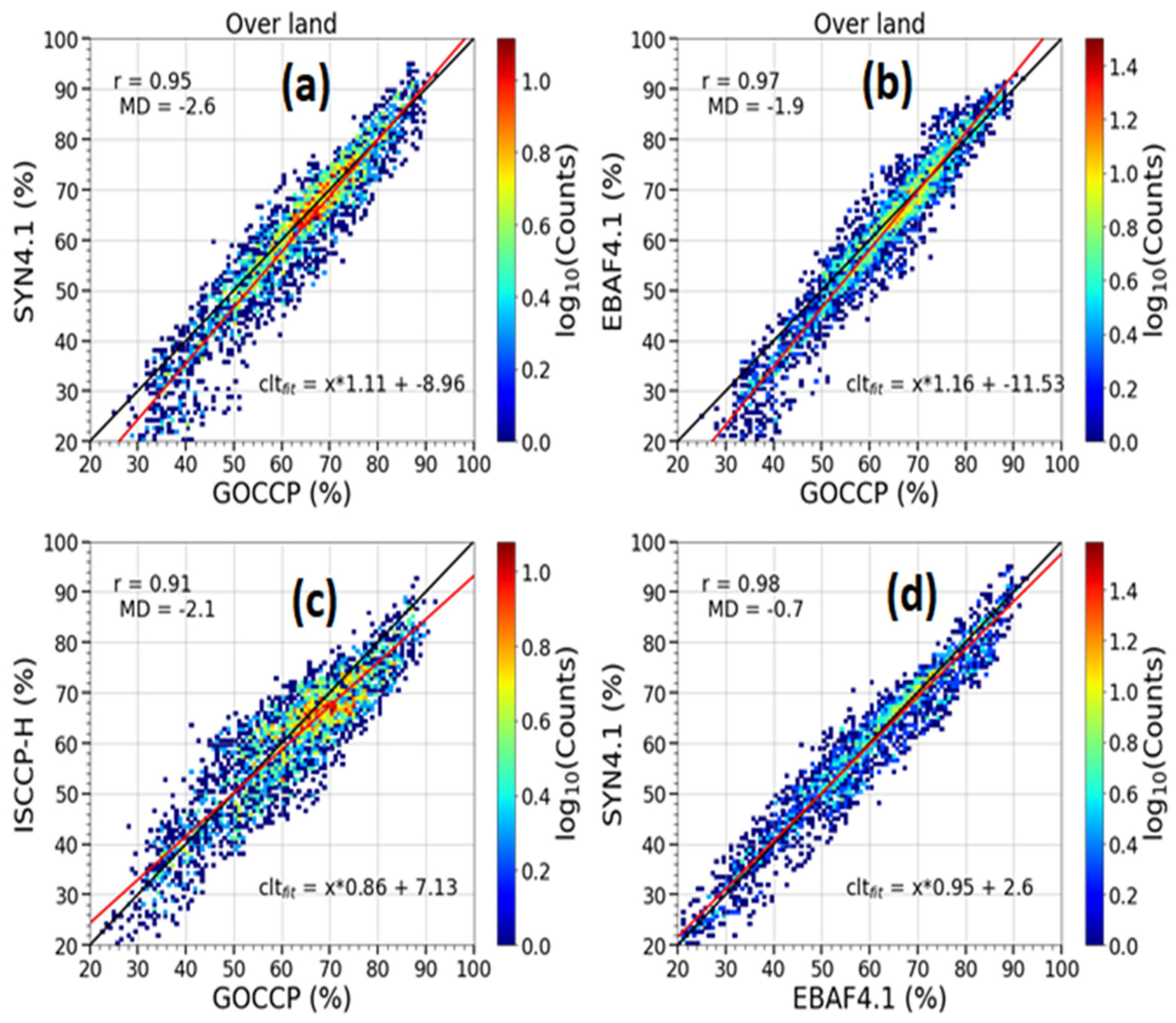
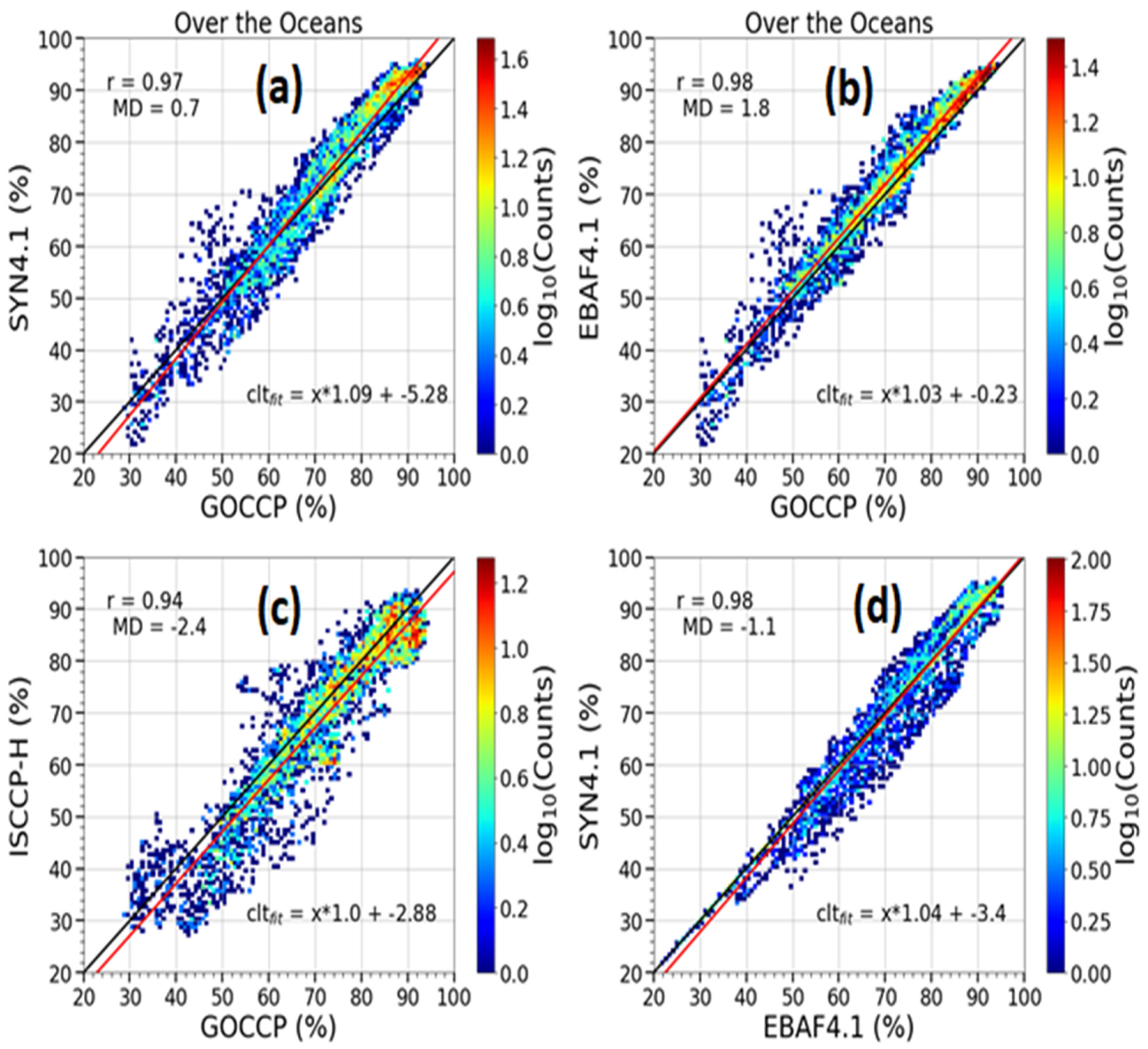
3.2. Comparisons over the Land and Oceanic Regions: 2D Density Plots

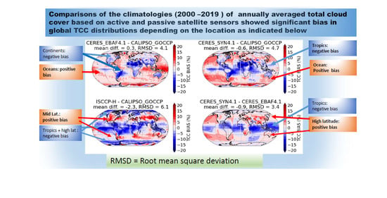
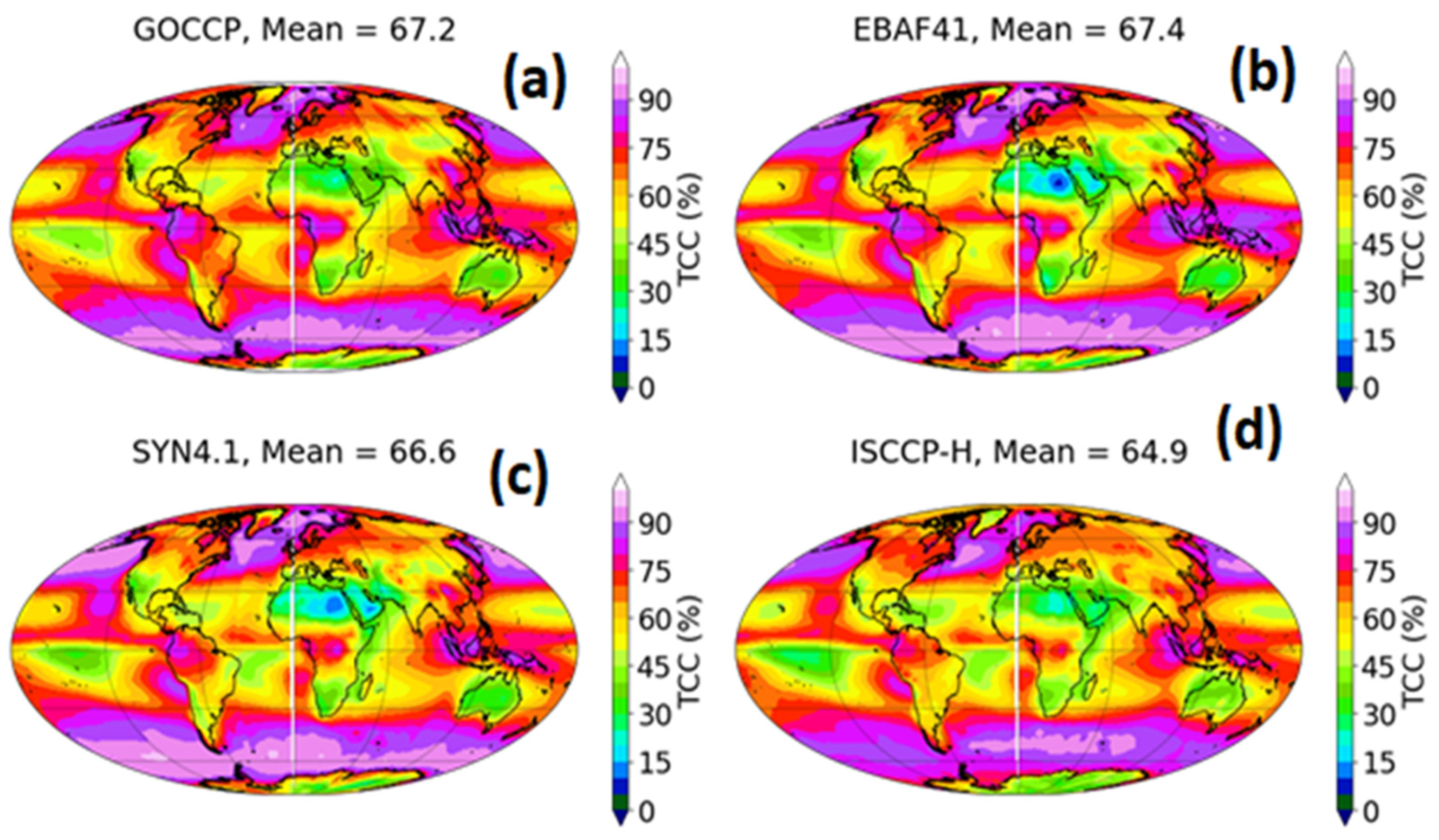
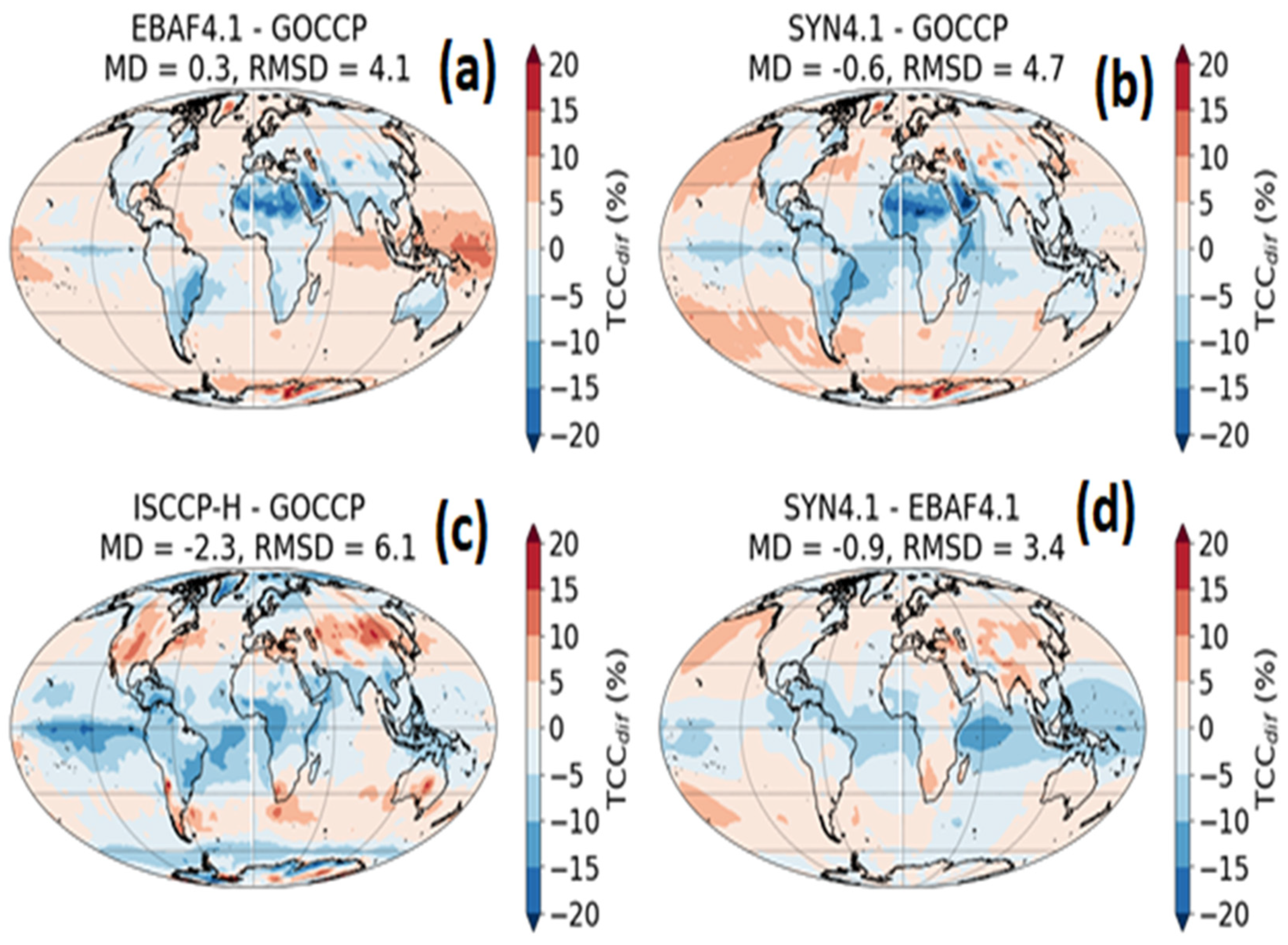
Figure 2 shows the comparisons of the TCC over land to the CALIPSO data. As indicated in the figure, over land, on average, all of the passive sensors underestimated the cloud cover as compared to the GOCCP relative to the combined data shown in Figure 1, particularly the SYN4.1 version of the CERES data, with a MD of −2.6% (a) followed by the EBAF4.1 and ISCCP-H data with a MD of near −2.0% ((a) and (b)). On the other hand, over the ocean, as depicted in Figure 3, the CERES-based passive sensors overestimated the cloud cover, particularly the EBAF4.1 (b). However, the SYN4.1 agreed with the GOCCP reasonably well (a). The ISCCP-H data underestimated the cloud cover under all surface conditions (Figure 1, Figure 2 and Figure 3). The discrepancy at lower cloud cover appeared to get better when the satellite data sets were compared over the ocean ((a) and (b)). This could be partly because most of the clouds over oceanic regions are optically thicker than over land where the passive sensors normally do better, which is consistent with previous studies [15]. The two CERES data sets agreed slightly better over land than over oceans.

3.3. Global Maps

Figure 4 shows global maps of annually averaged GOCCP (a), EBAF4.1 (b), SYN4.1 (c), and ISCC-H (d) TCC data. The area-weighted global mean TCC values were 67.2%, 67.4%, 66.6%, and 66% for GOCCP, EBAF4.1, SYN4.1, and ISCC-H, respectively, indicating that the values for GOCCP and EBAF4.1 were very similar and the SYN4.1 and ISCCP-H values were slightly smaller. For the oceanic regions, the mean values were higher, 71.3%, 73.1%, 72%, and 68.9%, and over land the values were smaller, 61.2%, 59.3%, 58.6%, and 59.1% for GOCCP, EBAF4.1, SYN4.1, and ISCC-H, respectively. The mean value based on the ISCC-H data was comparable to the other datasets over the continental regions, but smaller over the oceanic regions. The global mean values previously reported by [14] for the GOCCP data were identical to the values reported in this study. However, the values included in their report for the older version of the ISCCP data were 64%, 68%, and 56%, corresponding to over the global, ocean, and land, respectively, indicating relatively lower values as compared to the current ISCCP-H version of the data.

The visual inspection of Figure 4 indicates also that all the satellite data sets generally agreed, showing the typical climatological regions associated with the general atmospheric circulation by indicating enhanced clouds over the Inter Tropical Convergence Zone (ITCZ) and mid- and high-latitude storm track regions. There were also some quantitative differences between the passive (ISCCP-H and CERES products) and GOCCP datasets at certain geographical regions. The two CERES cloud products, the EBAF 4.1 and SYN4.1 ((b) and (c)), showed less cloud cover over the dry and dusty Sahelian region of northern Africa as compared to the GOCCP and ISCCP data. This was consistent with Figure 2, which showed that EBAF 4.1 and SYN 4.1 underestimated the cloud cover at lower TCC values (TCC < ~50%). This may be partly associated with some limitations of the passive sensors to discriminating clouds from dust as well as optically thin clouds. The ISCC-H data also showed lower TCC, but relatively agreed with the GOCCP data over these regions. On the other hand, the ISCCP-H data underestimated cloud cover over the southern hemisphere near 60° S, where the other data sets showed a significantly enhanced TCC. As will be discussed later, this area is dominated by LLC; thus, the ISCCP data appeared to fail at capturing some of the LLC in this part of the globe. The visual inspection also revealed that the ISCCP-H data showed relatively lower cloud cover in the tropics.

The differences between the TCC obtained based on the active and passive sensors are further shown in Figure 5, which shows the global maps of the bias in annually averaged TCC as compared to the GOCCP data and associated root mean square deviation (RMSD). As illustrated in the figure (a), the EBAF4.1 data agreed reasonably well with GOCCP, with a RMSD of 4.1%. The exceptions are over the Sahelian desert in northern Africa and southeastern South America, where the EBAF4.1 underestimated the cloud cover (10–20%) mostly over the continents. Based on this study, there is no evidence of misidentification of large aerosol particles as clouds over dusty, large, desert areas, as discussed in the data-quality summary [29]. In fact, EBAF4.1 overestimated the TCC (5–20%) over the Pacific Islands between the Indian and Western Pacific Ocean, where high level deep convective clouds are normally expected [33], and included a slight overestimation of cloud cover mainly over the oceanic regions of the globe. The SYN4.1 version of the satellite data (b) behaved very similarly to EBAF4.1 (a) when the data were compared to the GOCCP data. However, it underestimates the TCC much more severely over northern Africa and some parts of tropical regions. In contrast, this version of the CERES data overestimated the cloud cover over the northern and southern portions of the Pacific Ocean, but the data agreed with GOCCP data much better over the Pacific Islands as compared to EBAF4.1. The calculated RMSD for SYN4.1 was 4.7%, which is slightly higher as compared to EBAF4.1. As shown in (d), the ISCCP data showed less cloud cover when compared against the GOCCP data over the tropical regions, particularly over the southern Pacific and Atlantic Oceans near the equator and also over the polar regions, where the satellite retrieval using the passive sensors was generally much more challenging (c). In contrast, the ISCCP data overestimated the cloud cover between about 40° and 60° latitude in both hemispheres, particularly over North America and Europe, by about 5% and 10% depending on the location. This finding of the overestimation of the TCC over the European continent by the ISCCP-H data is consistent with the previous study [18] that compared the ISCCP data with surface-based measurements. The RMSD value for the ISCCP-H data was 6% higher than the CERES datasets. The comparisons of the CERES cloud product (d) revealed that the largest discrepancy occurred in the tropical oceans, where the EBAF4.1 data showed higher cloud cover and the calculated RMSD value was 3.4%. Based on these results, overall, the EBAF4.1 agreed with the GOCCP data better except over some parts of dry regions such as the Sahara Desert located in northern Africa.

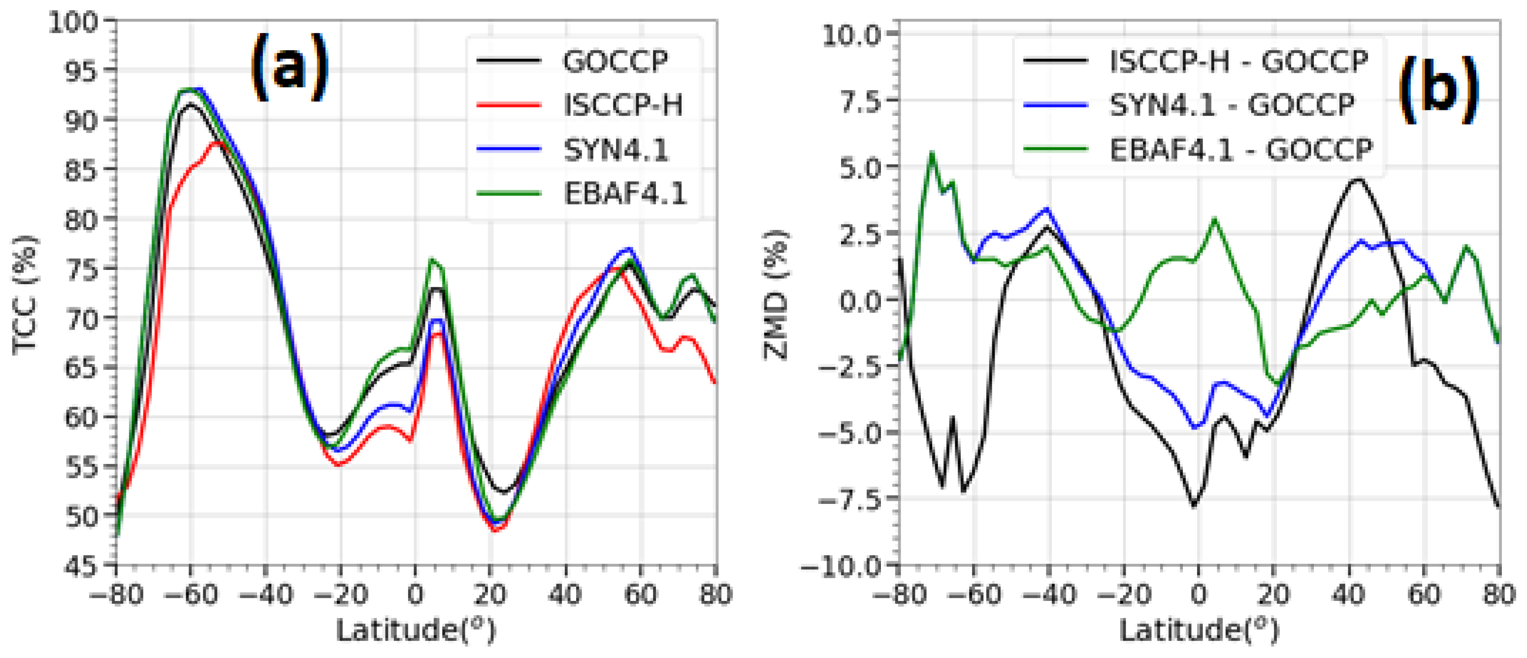
3.4. Annual and Zonal Means

The zonally and annually averaged satellite cloud products and associated zonal mean bias (ZMB) as compared to the GOCCP data are shown in Figure 6 ((a) and (b) respectively). Based on the zonal mean data perspectives ((a) and (b)), the EBAF4.1 data agreed relatively better with the GOCCP data as compared to the ISCCP-H and SYN4.1 datasets over all latitudes, with a slight overestimation of TCC near the equator (ZMD < 2.5%), possibly associated with the positive bias over regions such as the Pacific Islands and the northern Indian Ocean, and underestimation near the poles (latitude > 75° over both latitudes). Both the SYN4.1 and ISCCP-H data underestimated the TCC over the tropical latitudes (20° S and 20° N), with a maximum ZMD of −5%. In the mid-latitude portions of the globe, between 20° S and 60° S and 20° N and 80° N, the ZMDs were well below 2.5% for all data except the ISCCP-H that overestimated and underestimated the cloud cover with a maximum ZMD of −7.5% and 5%, respectively. It is particularly interesting to note that the ISCCP-H data significantly underestimated the cloud cover of high latitude regions (≈55° < latitude < 75°) in both hemispheres, with a maximum ZMD close to −7.5%. In these regions, the CERES products slightly overestimated the TCC. It is worth noting that over these regions, the ISCCP uses the polar orbiting satellite to retrieve the TCC. The ISCCP-H data actually slightly overestimated the TCC near the south polar regions (latitude > 75°), also contrary to the CERES products (b). These parts of the globe are generally difficult for the passive sensors to retrieve reliable cloud data as compared the active sensors. However, as mentioned earlier, there are some uncertainties also in the active remote sensing. Nonetheless, according to these results, the ISCC-H data were more significantly affected at high latitude regions as compared to the CERES datasets.

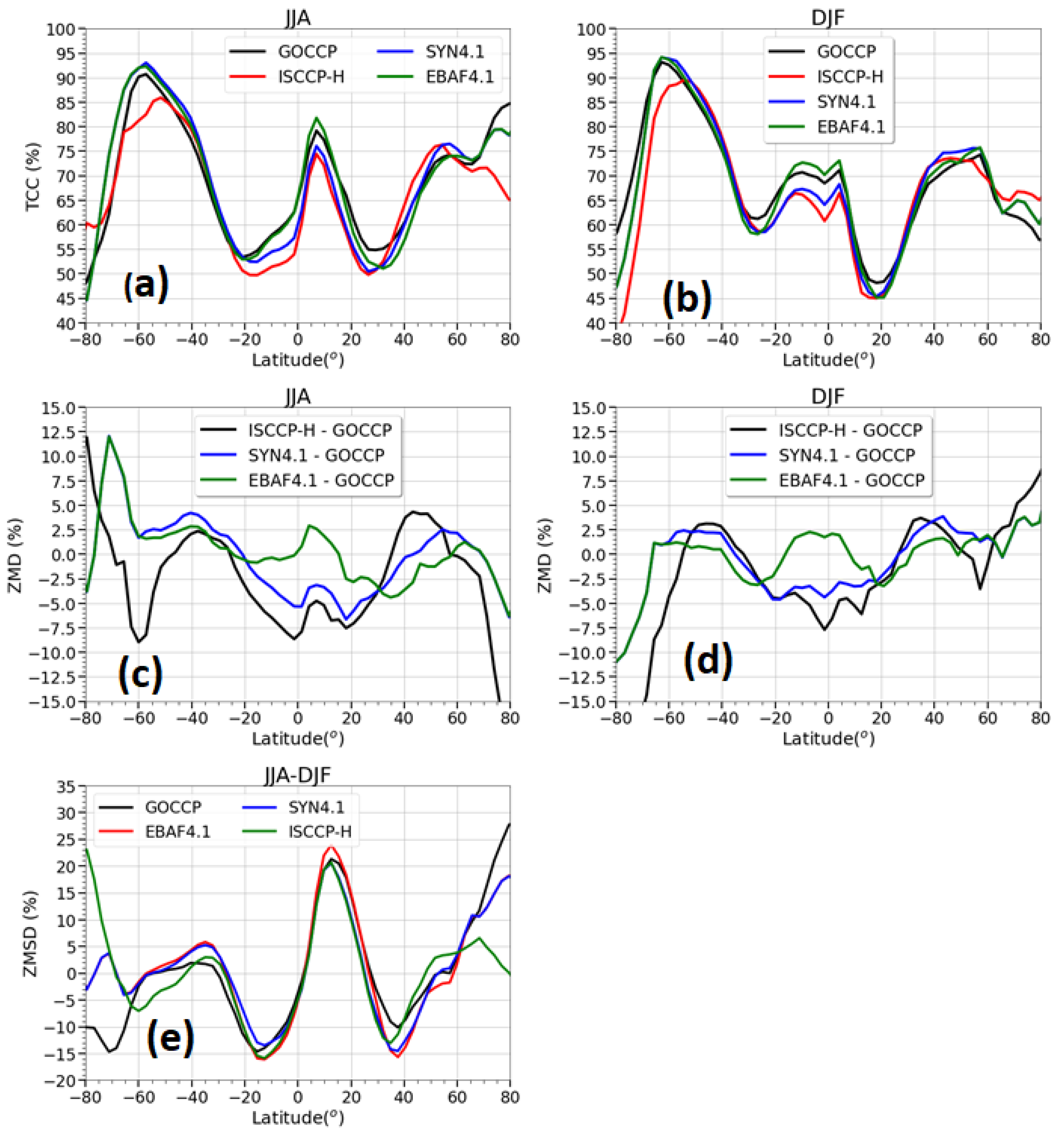
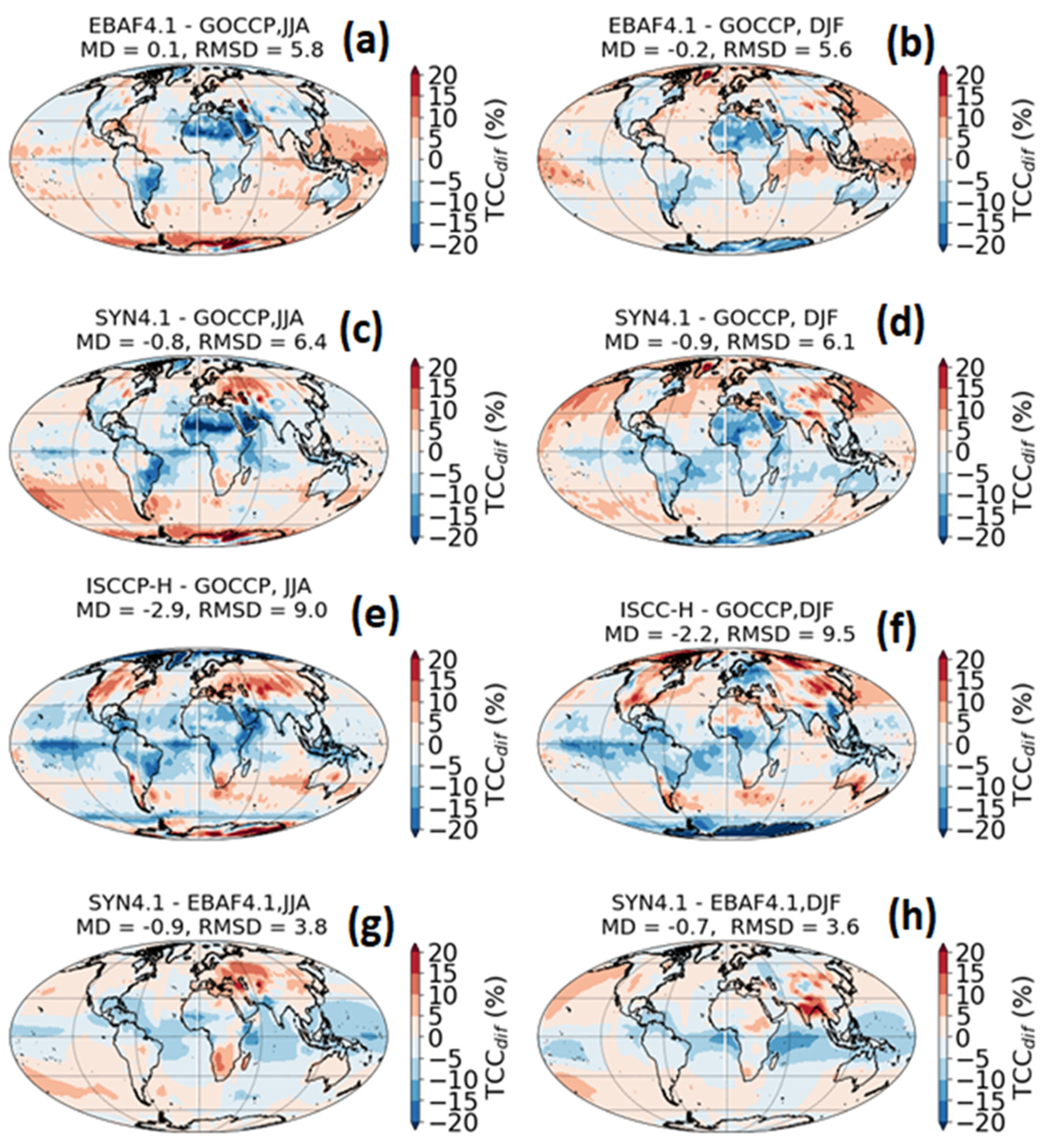
3.5. Seasonal Climatology Comparisons

Figure 7 shows the global maps of annually and seasonally averaged bias in TCC and RMSD as compared to the CALIPSO data. The first and second columns show the northern hemisphere summer (JJA) and winter (DJF) seasons, respectively. Generally, the CERES data sets are characterized by significant positive bias in the winter hemisphere over the oceanic regions, reaching a maximum close to 15% over the Western Pacific (both hemispheres) and negative bias in the summer hemisphere, particularly over the continents including the Antarctic and Sahelian regions, with a maximum bias of close to −15% ((a), (b), (c), and (d)). From a global mean perspective, the EBAF4.1 slightly overestimated and underestimated the TCC during JJA and DJF seasons, with MD values of 0.1% and −0.2%, respectively ((a) and (b)). The RMSD values for EBAF4.1 were 5.8% and 5.6% for JJA and DJF, respectively. Overall, during the summer hemisphere, the CERES data sets reasonably agreed with the GOCCP data over the oceanic regions than over the continents. The bias in the ISCCP-H data had similar behavior, but a notable exception is the area of large negative bias, reaching −15% to −20% in the tropics and around the globe near the 60° S during the JJA season, expanded towards the South Pole during the DJF season ((e) and (f)). The seasonal variation of the difference between the two CERES TCC products (EBAF4.1 and SYN4.1) was not as high as when we compared with the GOCCP data; but EBAF4.1 produces more clouds (positive bias ≈ 5%) in the tropics during both seasons, having a slightly wider positive bias during the northern hemisphere summer ((g) and (h)). Thus, according to these results, the passive sensors significantly underestimated cloud cover during summer in both hemispheres.

Figure 8 shows zonally and seasonally averaged TCC JJA ((a)) and DJF (b) based on the GOCCP, EBAF4.1, SYN4.1, and ISCCP-H data and the associated bias for each season with respect of the GOCCP data (panes c and d). The variability of zonally and seasonally averaged TCC looks very similar to Figure 6. However, the exceptions are the cloud locations associated with the Hadley circulation and mid-latitude storm tracks, which moved towards the northern hemisphere during the northern hemisphere summer, as obviously would be expected ((a) and (b)). Over the oceans (latitude > 20°S) in the southern hemisphere during the southern hemisphere winter (JJA), the CERES cloud products overestimated the cloud cover (positive bias) as compared to the CLAPISO data. In contrast, the ISCCP-H data significantly underestimated the cloud near the latitude 60°S, as already discussed earlier. Similar behavior can be seen during the northern hemisphere winter. Based on zonally and seasonally averaged data, during the summer season in both hemispheres, all the satellite products based on the passive sensors underestimated the cloud cover at higher latitudes (latitude > 60°S and 60°N), particularly the ISCCP-H data (see (c) and (d)). In the tropical region, both ISCCP-H and SYN4.1 underestimated the cloud cover during both the summer and winter seasons, with values varying between −2.5% to −7.5% ((c) and (d)). As mentioned earlier, Figure 8 also reveals that the EBAF4.1 data agreed with GOCCP data within the latitude 60°S and 60°N relatively better than the other satellite products in both summer and winter seasons. According to Figure 8e, all of the satellite products exhibited significant inter-seasonal variability (JJA-DJF) over the tropics (between 20°S and 40°N) and polar regions as a result of the movements of Hadley cells and strong seasonal variability of polar regions, respectively. All the satellite products showed similar variability in the tropics, with zonal mean seasonal difference (ZMSD) between −15% in the south and about 20% in the north, except the EBAF4.1 data that showed relatively higher variability (−15% to 25%). In the high latitudes regions (poleward of 60° in both hemispheres), however, the GOCCP retrieval produced higher TCC in the northern hemisphere and lower TTC in the southern hemi-sphere during the JJA season. The CERES products (ENAF4.1 and SYN4.1) followed a similar trend as the GOCCP in the northern hemisphere, but deviated somewhat in the southern hemisphere polar regions. In contrary, the ISCCP-H showed relatively smaller variability between JJA and DJF seasons in the northern hemisphere; but, over the southern hemisphere, it produced significantly higher TCC in JJA as compared to the DJF season, reaching close to a 23% difference near 80° S. There was No significant inter-seasonal variability over the southern hemisphere (30° S–60° S). This may be because the area is mainly dominated by oceans. According to these results, all of the data sets had higher TCC over the polar regions during the JJA season except the GOCCP data over the southern hemisphere, which showed relatively lower TCC. Based on CloudSat/CALIPSO data, [34] also showed a similar seasonal trend as the GOCCP data. This can be explained based on (a) and (b) in Figure 8 that show that all the passive sensors reported higher TCC near the south pole (north of 70° S) during JJA (southern hemisphere winter) as compared to the DJF season (southern hemisphere summer). However, as stated above, this was not supported by the active sensor.

4. Summary and Conclusions

In this study, the climatologies of four different satellite cloud products based on an active senor (CAPLISO-GOCCP; hereafter, GOCCP) and passive sensors from CERES (versions EBAF4.1 and SYN4.1) and from ISCCP-H were compared. These comparisons were carried out over the entire globe (ocean + land) and separately over the oceans and continental regions. The statistical comparisons of the annually averaged monthly mean total cloud cover (TCC) retrieved over the entire globe based on the passive and active sensors revealed that the correlation coefficient (r) between the two types of measurements was well over 0.93. Based on a monthly averaged data perspective, the two CERES cloud products, SYN4.1 and EBAF4.1, on average slightly underestimated and overestimated the TCC compared to the GOCCP, having a mid-difference (MD) of −0.6% and 0.3%, respectively. The ISCCP-H version of the data generally underestimated the TCC as compared to the GOCCP data by a relatively higher MD value of −2.3%. Most of the discrepancies between the GOCCP and CERES data sets occurred at lower cloud covers (TCC < 50%) where the CERES datasets significantly underestimated the TCC. The two CERES products, EBAF4.1 and SYN4.1, showed excellent agreement with each other with a correlation coefficient of r = 0.98. However, on average, the EBAF4.1 data were larger by about 1%. Over the land areas, all of the passive sensors underestimated the cloud cover as compared to the GOCCP relative to the combined data (land + ocean), particularly the SYN4.1 version of the CERES data, with a MD of −2.6% followed by the EBAF4.1 and ISCCP-H data with a MD of approximately −2.0%. Over the ocean, the CERES-based passive sensors overestimated the cloud cover, particularly the EBAF4.1; but the SYN4.1 agreed with the CALIPSO reasonably well. The ISCCP-H data underestimated the cloud cover under all surface conditions.

Comparisons of the global maps of annually averaged TCC from the passive sensors against the corresponding active sensor data generally showed that all of the products captured similar climatologies of the TCC distributions but with some differences over various geographical regions in the tropics, such as the Sahelian region of northern Africa, where the CERES data sets underestimated the TCC as compared to the GOCCP data. The ISCC-H data also showed lower TCC over this region as well as over the tropics, particularly over the southern hemisphere near 60° S, where the other data sets showed a significantly enhanced TCC. The exceptions were over northern Africa and southeastern South America, where the EBAF4.1 underestimated the cloud cover (10–20%) mostly over the continents and also over the Pacific Islands between the Indian and eastern Pacific Oceans, where EBAF4.1 overestimated the cloud cover (5–20%). The ISCCP data overestimated the TCC between about 40° and 60° latitude in both hemispheres, particularly over North America and Europe by about 5% and 10% depending on the location. The global distribution of the bias between the active and passive sensors also showed that the EBAF4.1 TCC data agreed reasonably well with GOCCP, with a root mean square deviation (RMSD) of 4.1% as compared to 6% for ISCCP-H data. All of the products had higher seasonal RMSD values as compared to the annual mean data.

From zonally and annually averaged TCC perspectives, the EBAF4.1 data also agreed relatively better with the GOCCP data over all latitudes as compared to the other satellite datasets, particularly within the latitudes (60°S and 60°N) where the zonal mean difference (ZMD) varied between ±2.5% with a slight overestimation of TCC near the equator and near the poles. Both the SYN4.1 and ISCCP-H data underestimated the cloud cover over the tropical latitudes (20°S and 20°N).

According to these results, the comparisons of the spatial distribution and climatological variability of the TCC retrieved using the passive sensors (EBAF4.1, SYN4.1, and ISCCP-H) against the GOCCP data depended on the geographical locations as well as the associated algorithm used. As discussed above, the TCC retrieved using the passive sensors agreed with each other and also as compared to the GOCCP data over some geographical locations. Hence, in these regions, the data obtained using the passive sensors can be used with some confidence. According to this study, the CERES EBAF4.1 data in particular reasonably agreed with the GOCCP data over a number of geographical regions. However, based on these results, the use of the ICCP data, particularly in the tropics and some high latitude regions, is questionable. Further in-depth study is required to get better insights into these discrepancies.

References

1. Boucher, O.; Randall, D.; Artaxo, P.; Bretherton, C.; Feingold, G.; Forster, P.; Kerminen, V.-M.; Kondo, Y.; Liao, H.; Lohmann, U.; et al. Clouds and Aerosols. In Climate Change 2013: The Physical Science Basis. Contribution of Working Group I to the Fifth Assessment Report of the Intergovernmental Panel on Climate Change; Stocker, T.F., Qin, D., Plattner, G.-K., Tignor, M., Allen, S.K., Boschung, J., Nauels, A., Xia, Y., Bex, V., Midgley, P.M., Eds.; Cambridge University Press: Cambridge, UK; New York, NY, USA, 2013. [Google Scholar]
2. Pachauri, R.K.; Allen, M.R.; Barros, V.R.; Broome, J.; Cramer, W.; Christ, R.; Church, J.A.; Clarke, L.; Dahe, Q.; Dasgupta, P. Climate Change 2014: Synthesis Report. Contribution of Working Groups I, II and III to the Fifth Assessment Report of the Intergovernmental Panel on Climate Change; Pachauri, R.K., Meyer, L.A., Eds.; IPCC: Geneva, Switzerland, 2014; p. 151. [Google Scholar]
3. Zelinka, M.D.; Randall, D.A.; Webb, M.J.; Klein, S.A. Clearing clouds of uncertainty. Nat. Clim. Chang. 2017, 7, 674–678. [Google Scholar] [CrossRef]
4. Wyser, K.; von Noije, T.; Yang, S.; von Hardenberg, J.; O’Donnell, D.; Döscher, R. On the increased climate sensitivity in the EC-Earth model from CMIP5 to CMIP6. Geophys. Model Dev. 2020, 13, 3465–3474. [Google Scholar] [CrossRef]
5. Meehl, G.A.; Senior, A.C.; Eyring, V.; Flato, G.; Lamarque, J.-F.; Stouffer, R.J.; Taylor, K.E.; Schlund, M. Context for interpreting equilibrium climate sensitivity and transient climate response from the CMIP6 Earth system models. Sci. Adv. 2020, 6, eaba1981. [Google Scholar] [CrossRef] [PubMed]
6. Swart, N.C.; Cole, J.N.S.; Kharin, V.V.; Lazare, M.; Scinocca, J.F.; Gillett, N.P.; Anstey, J.; Arora, V.; Christian, J.R.; Hanna, S.; et al. The Canadian Earth System Model version 5 (CanESM5.0.3). Geosci. Model Dev. 2019, 12, 4823–4873. [Google Scholar] [CrossRef] [Green Version]
7. Zelinka, M.D.; Myers, T.A.; McCoy, D.T.; Po-Chedley, S.; Caldwell, P.M.; Ceppi, P.; Klein, S.A.; Taylor, K.E. Causes of higher climate sensitivity in CMIP6 models. Geophys. Res. Lett. 2020, 47, e2019GL085782. [Google Scholar] [CrossRef] [Green Version]
8. Ceppi, P.; Brient, F.; Zelinka, M.D.; Hartmann, D.L. Advanced Review Cloud feedback mechanisms and their representation in global climate models. Wiley Interdiscip. Rev. Clim. Chang. 2017, 8, e465. [Google Scholar] [CrossRef]
9. Evan, A.T.; Heidinger, A.K.; Vimont, D.J. Arguments against a physical long-term trend in global ISCCP cloud Amounts. Geophys. Res. Lett. 2007, 34, L04701. [Google Scholar] [CrossRef]
10. Norris, J.R.; Allen, R.J.; Evan, A.T.; Zelinka, M.D.; O’Dell, C.W.; Klein, S.A. Evidence for climate change in the satellite cloud record. Nature 2016, 536, 72–75. [Google Scholar] [CrossRef] [Green Version]
11. Vignesh, P.P.; Jiang, J.H.; Kishore, P.; Su, H.; Smay, T.; Brighton, N.; Velicogna, I. Assessment of CMIP6 cloud cover and comparison with satellite observations. Earth Space Sci. 2020, 7, e2019EA000975. [Google Scholar] [CrossRef]
12. Wang, T.; Fetzer, E.J.; Wong, S.; Kahn, B.H.; Yue, Q. Validation of MODIS cloud mask and multilayer flag using CloudSat-CALIPSO cloud profiles and a cross-reference of their cloud classifications. J. Geophys. Res. Atmos. 2016, 121, 11620–11635. [Google Scholar] [CrossRef]
13. Trepte, Q.Z.; Minnis, P.; Sun-Mack, S.; Yost, C.R.; Chen, Y.; Jin, Z.; Hong, G.; Chang, F.-L.; Smith, W.L.; Bedka, K.M.; et al. Global Cloud Detection for CERES Edition 4 UsingTerra and Aqua MODIS Data. IEEE Trans. Geosci. Remote Sens. 2019, 57, 9410–9448. [Google Scholar] [CrossRef]
14. Stubenrauch, C.J.; Rossow, W.B.; Kinne, S. Assessment of global cloud datasets from satellites: A project of the World Climate Research Programme Global Energy and Water Cycle Experiment (GEWEX) Radiation Panel. WCRP Rep. 2012, 23, 176. [Google Scholar]
15. Noel, V.; Chepfer, H.; Chiriaco, M.; Winker, D.; Okamoto, H.; Hagihara, Y.; Cesana, G. Disagreement among global cloud distributions from CALIOP, passive satellite sensors and general circulation models. insu-01735143. 2018. Available online: https://hal-insu.archives-ouvertes.fr/insu-01735143 (accessed on 13 December 2021).
16. Chepfer, H.; Cesana, G.; Winker, D.; Getzewich, B.; Vaughan, M.; Liu, Z. Comparison of Two Different Cloud Climatologies Derived from CALIOP-Attenuated Backscattered Measurements (Level 1): The CALIPSO-ST and the CALIPSO-GOCCP. J. Atmos. Ocean. Technol. 2013, 30, 725–744. [Google Scholar] [CrossRef] [Green Version]
17. Lacour, A.; Chepfer, H.; Shupe, M.D.; Miller, N.B.; Noel, V.; Kay, J.; Turner, D.D.; Guzman, R. Greenland Clouds Observed in CALIPSO-GOCCP: Comparison with Ground-Based Summit Observations. J. Clim. 2017, 30, 6065–6083. [Google Scholar] [CrossRef]
18. Tzallas, V.; Hatzianastassiou, N.; Benas, N.; Meirink, J.F.; Matsoukas, C.; Stackhouse, P., Jr.; Vardavas, I. Evaluation of CLARA-A2 and ISCCP-H Cloud Cover Climate Data Records over Europe with ECA&D Ground-Based Measurements. Remote Sens. 2019, 11, 212. [Google Scholar]
19. Jones, P.W. First- and second-order conservative remapping schemes for grids in spherical coordinates. Mon. Weather Rev. 1999, 127, 2204–2210. [Google Scholar] [CrossRef]
20. Rossow, W.B.; Schiffer, R.A. ISCCP cloud data products. Bull. Am. Meteorol. Soc. 1991, 71, 2–20. [Google Scholar] [CrossRef]
21. Rossow, W.B.; Schiffer, R.A. Advances in understanding clouds from ISCCP. Bull. Am. Meteorol. Soc. 1999, 80, 2261–2287. [Google Scholar] [CrossRef] [Green Version]
22. Young, A.H.; Knapp, K.R.; Lnamdar, A.; Hankins, W.; Rossow, W.B. The International Satellite Cloud Climatology Project H-Series climate data record product. Earth Syst. Sci. Data 2018, 10, 583–593. [Google Scholar] [CrossRef] [Green Version]
23. Knapp, R.K.; Young, A.H.; Semunegus, H.; Inamdar, A.K.; Hankins, W. Adjusting ISCCP Cloud Detection to Increase Consistency of Cloud Amount and Reduce Artifacts. J. Atmos. Ocean. Technol. 2021, 38, 155–165. [Google Scholar] [CrossRef]
24. Chepfer, H.; Bony, S.; Winker, D.M.; Cesana, G.; Dufresne, J.L.; Minnis, P.; Stubenrauch, C.J.; Zeng, S. The GCM Oriented CALIPSO Cloud Product (CALIPSO-GOCCP). J. Geophys. Res. 2010, 115, D00H16. [Google Scholar] [CrossRef]
25. Bodas-Salcedo, A.; Webb, M.J.; Bony, S.; Chepfer, H.; Dufresne, J.-L.; Klein, S.A.; Zhang, Y.; Marchand, R.; Haynes, J.M.; Pincus, R.; et al. COSP: Satellite simulation software for model assessment. Bull. Am. Meteorol. Soc. 2011, 92, 1023–1043. [Google Scholar] [CrossRef]
26. Swales, D.J.; Pincus, R.; Bodas-Salcedo, A. The Cloud Feedback Model Intercomparison Project Observational Simulator Package: Version 2. Geosci. Model Dev. 2018, 11, 77–81. [Google Scholar] [CrossRef] [Green Version]
27. Cesana, G.; Chepfer, H. Evaluation of the cloud thermodynamic phase in a climate model using CALIPSO-GOCCP. J. Geophys. Res. Atmos. 2013, 118, 7922–7937. [Google Scholar] [CrossRef]
28. Hogan, R.J.; Francis, P.N.; Flentje, H.; Illingworth, A.J.; Quante, M.; Pelon, J. Characteristics of mixed-phase clouds. I: Lidar, radar and aircraft observations from CLARE’98. Q. J. R. Meteorol. Soc. 2003, 129, 2089–2116. [Google Scholar] [CrossRef] [Green Version]
29. CERES_EBAF_Ed4.1 Data Quality Summary. Available online: https://ceres.larc.nasa.gov/documents/DQ_summaries/CERES_EBAF_Ed4.1_DQS.pdf (accessed on 13 December 2021).
30. CERES_SSF_Terra-Aqua_Edition4A Data Quality Summary. Available online: https://asdc.larc.nasa.gov/documents/ceres/quality_summaries/CER_SSF_Terra-Aqua_Edition4A.pdf (accessed on 13 December 2021).
31. Minnis, P.; Sun-Mack, S.; Young, D.F.; Heck, P.W.; Garber, D.P.; Chen, Y.; Spangenberg, D.A.; Arduini, R.F.; Trepte, Q.Z.; Smith, W.L.; et al. CERES Edition-2 cloud property retrievals using TRMM VIRS and Terra and Aqua MODIS data, Part I: Algorithms. IEEE Trans. Geosci. Remote. Sens. 2011, 49, 4374–4400. [Google Scholar] [CrossRef]
32. CERES_SYN1deg_Ed4A Data Quality Summary. Available online: https://ceres.larc.nasa.gov/documents/DQ_summaries/CERES_SYN1deg_Ed4A_DQS.pdf (accessed on 13 December 2021).
33. Gettelman, A.; Salby, M.L.; Sassi, F. Distribution and influence of convection in the tropical tropopause region. J. Geophys. Res. 2002, 107, 4080. [Google Scholar] [CrossRef]
34. Bromwich, D.H.; Nicolas, J.P.; Hines, K.M.; Kay, J.E.; Key, E.L.; Lazzara, M.A.; Lubin, D.; McFarquhar, G.M.; Gorodetskaya, I.V.; Grosvenor, D.P.; et al. Tropospheric clouds in Antarctica. Rev. Geophys. 2012, 50, RG1004. [Google Scholar] [CrossRef] [Green Version]
Figure 1. The 2D density plots of annually averaged TCC obtained based on EBAF4.1 (a), SYN4.1 (b), and ISCCP-H (c), and against the TCC obtained from the GOCCP-CALIPSO satellite. Comparison of the two CERES products, EBAF4.1 and SYN4.1, is shown in the fourth column (d). The red lines represent the linear fit equations also shown.
Remotesensing 13 05150 g001
Figure 2. The same as Figure 1, but over the continental regions.
Remotesensing 13 05150 g002
Figure 3. The same as Figure 1, but over the oceanic regions.
Remotesensing 13 05150 g003
Figure 4. Global maps of annually averaged TCC based on GOCCP-CALIPSO (a), EBAF4.1 (b), SYN4.1 (c), and ISCCP-H (d).
Remotesensing 13 05150 g004
Figure 5. Global maps of bias (x-GOCCP) in annually averaged TCC and root mean square deviation (RMSD) where x represents EBAF4.1 (a), SYN4.1 (b), ISCCP-H (c), and EBAF4.1–SYN4.1 (d).
Remotesensing 13 05150 g005
Figure 6. Annually zonally averaged TCC (a) and the zonal mean differences (ZMD) (b).
Remotesensing 13 05150 g006
Figure 7. Global maps of bias of annually and seasonally averaged TCC and root mean square deviation (RMSD).
Remotesensing 13 05150 g007
Figure 8. Zonally and seasonally averaged TCC for summer (JJA) ( a) and winter (DJF) (b), zonal mean difference (ZMD) between active and passive sensors for JJA (c) and for DJF (d), and zonal mean seasonal difference (ZMSD) (JJA-DJF) (e).
Remotesensing 13 05150 g008