1. Introduction
Ceiling and visibility are two of the most important weather elements responsible for severe weather hazards for aviation. At least 29% of aviation accidents that occurred during the 2000–2011 period can be attributed to weather [
1]. Based on data collected between 2009 and 2013 by the US Federal Aviation Agency (FAA), low ceiling and visibility conditions are responsible for over 27% of weather-related aviation accidents and 70% of fatalities [
2]. Accuracy and calibration of instruments that measure visibility (VIS), cloud ceiling, relative humidity (RH), and temperature (T) are very important for accurate nowcasting and forecasting of visibility and cloud ceiling. These parameters also have critical importance for the validation of numerical weather prediction (NWP) and climate models. Based on a number of climate model simulations, on average, atmospheric absolute humidity is expected to increase in response to the increase in anthropogenic greenhouse gases and the associated increase in temperature [
3,
4,
5]. This is particularly true in the upper troposphere, where water vapor plays a significant role in the global radiation budget as a greenhouse gas [
4]. Since RH is defined as the ratio of the amount of water vapor (q
v) to the maximum amount expected at a given T when the atmosphere is saturated (q
s (T)), the effect of increasing both q
v and q
s has a compensating effect on RH. As a result, the observed global change in surface RH during 1976–2004 was relatively small (≈0.6%) [
6] and thus requires accurate measurements to be detected. At the surface level, RH is also used for visibility prediction applications (e.g., [
7,
8]).
Currently, standalone meteorological sensors are being used autonomously in some airports and remote locations. However, there have been limited studies of the accuracy of these instruments or how they compare with human observation. Data collected using the Vaisala FD12P sensor and human observation in southern Ontario [
7] showed that, on average, human observers record higher VIS values by about 20% compared to measurements (VIS < 15 km) obtained using optical probes, with a mean difference (MD) of about 700 m. They also found that the Rotronic RH/T sensor underestimated the RH near the saturation point when compared with more standard instruments, such as the AES-Dewcell instrument that will be described in the following section.
The purpose of this study was to test, validate, and estimate uncertainties of a number of commonly used ground-based and remote-sensing instruments based on observations collected using well-established standard reference instruments and human-based observations. To achieve this, two years (2015–2016) of surface observation data, collected as part of the 4Wing Cold Lake Research project during 2015–2016 at Cold Lake, Alberta, was used. The remainder of the paper is organized as follows. In
Section 2 the materials and methods are discussed, the results of the data analysis are given in
Section 3, and the summary and conclusions are given in
Section 4.
2. Materials and Methods
2.1. Study Area
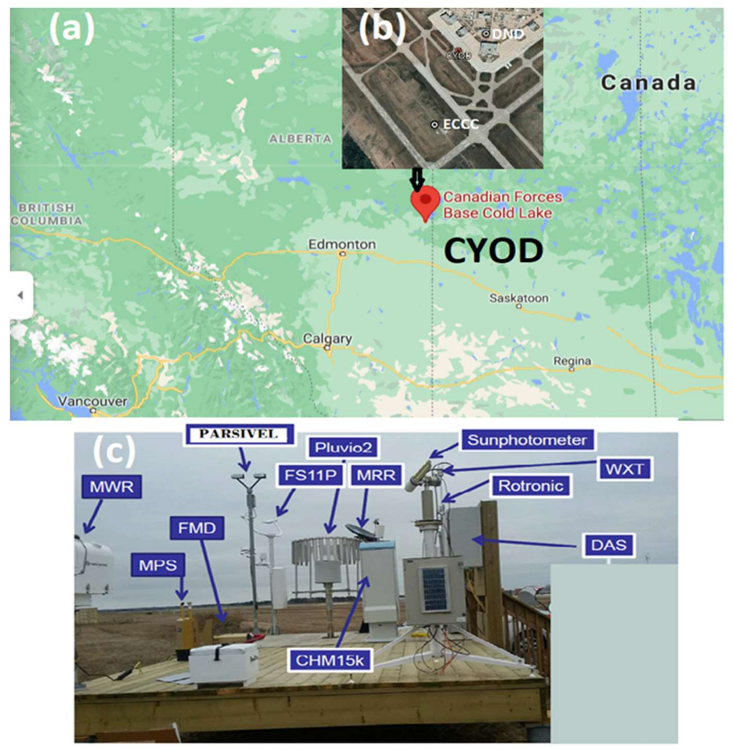
The study area (
Figure 1), the Cold Lake Regional Airport (CYOD), is located in northeastern Alberta, Canada (at 541 m MSL; 54 N, 110 W). In addition to the special ECCC observation site used in this study, there is a collocated permanent meteorological hourly observation (METAR) site used by the Canadian Department of National Defense (DND) within the CYOD airport, as indicated in the figure. The region is generally characterized by a humid continental climate with warm summers and cold winters [
9,
10]. To the west and northwest of the airport, there are four small lakes (Marie, Ethel, Crane, and Hilda), and to the northeast of the airport, two large lakes (Cold Lake and Primrose Lake) are known to contribute to the moistening of the atmosphere and affect the formation of precipitation and other weather phenomena when the flow is north-easterly. The west and southwest sides of the airport are surrounded by the Beaver River valley with an east–west orientation, which is also known to contribute various weather conditions including fog and lower ceilings and visibilities at the airport [
9,
10]. More discussions about the meteorological conditions of the location are given in
Section 3.
2.2. Instruments and Data
The meteorological instruments used in this study are shown in
Figure 1c. They include the Jenoptik CHM15k ceilometer, the Vaisala FS11P, and PWD22 present weather sensors, which measure VIS, precipitation intensity and type, and the radiometric, microwave radiometer (MWR) model MP-3000A, which measures cloud base height (CBH) and RH. The RH and T measured using the Vaisala WXT520 and AES-Dewcell sensors at the ECCC and DND site, respectively, were also used in the analysis (see
Figure 1b). The complete descriptions of the instruments are given in [
9,
10]. Here, we will briefly discuss the instruments.
The MP-3000A MWR is equipped with one zenith infrared (9.6–11.5 μm) sensor that retrieves cloud base brightness temperatures from which the CBH can be determined. The radiometer also incorporates measurements of RH and T at the ground level, using the Rotronic RH/T sensor, into its atmospheric profiling algorithms [
11]. The RH and T were also measured using another Rotronic HygroMet MP102 RH/T sensor. The HygroMet MP measures RH with a ROTRONIC Hygromer
® IN1 capacitive sensor and T with a Pt100 resistance temperature detector (RTD). Based on the manufacturer’s data sheet, the accuracy of these sensors at 23 °C is given as ±0.8% and ±0.1 °C.
The Vaisala WXT520 measures T and RH. The instrument is equipped with a capacitive ceramic THEMOCAP sensor for measuring air T and a capacitive thin film polymer HUMICAP180 sensor for RH measurements. According to the data given by the manufacturer, the accuracy of the WXT520 for measuring T is ±0.3 °C (for −52 °C < T < 60 °C), and the accuracy for measuring RH varies based on the measured RH (±3 for 0 < RH < 90%) and ±5% for 90 < RH < 100%).
As discussed earlier, the RH and T were also measured at the DND site, which is approximately 948 m away from the ECCC site (see
Figure 1b). The instrument used to measure RH and T at the DND site is the Atmospheric Environment Service (AES) Remote Temperature and Dewpoint Measuring Dewcell System Type 2, which is housed in a Stevenson screen. This is the standard instrument used operationally in Canada at weather stations, including those at major airports [
12,
13,
14]. A Dewcell measures Td with a temperature sensor covered with a wick soaked in a solution of lithium chloride, which is heated until its vapor pressure is in equilibrium with the ambient air. Using measurements of the T and T
d, the RH can be calculated. This sensor is designed to operate between −80 °C and 60 °C. The accuracy of the Dewcell measuring T
d is close to ±0.5 °C [
15,
16]. At colder temperatures (T
d < −10 °C), the accuracy is estimated to be lower (±1.5 °C) [
14]. The sensor is also checked for accuracy every week by comparing the reading to that of a reading taken from a psychrometer, which is also housed in a ventilated Stevenson screen. Acceptable accuracy with temperatures above 0 °C is up to ±1.0 °C for both the temperature and the dewpoint, and for temperatures below 0 °C, accuracy is up to ±2.0 °C. If the Dewcell is out of these tolerances, it must be taken out of service and properly cleaned and a minimum of three comparisons taken to ensure accuracy. Thus, the DND site Dewcell is a good instrument to calibrate and validate other sensors that are normally factory calibrated and not regularly checked for accuracy.
The Vaisala PWD22 and FS11P sensors measure precipitation, precipitation type, and visibility based on a forward light scattering principle with some minor difference in the scattering angle utilized. Both probes have similar configurations with two arms, one with a near-infrared transmitter and the other with a receiver. The two arms are aligned at certain angle so that the receiver can capture the scattered light if it is forward scattered at a given angle. In case of the PWD22, the angle is set at 45°; for the FS11P, the angle is 42°. These instruments are also equipped with a heated capacitive surface that captures falling precipitation particles and evaporates them to obtain a liquid water equivalent measurement. The precipitation intensity and type are obtained by means of signal processing software that analyzes the voltage output from the receiver, along with the current temperature. Using a proprietary algorithm, the sensors calculate VIS using the measured extinction (Ext) (VIS = 3/Ext) and an assumed threshold for visual contrast based on an equation derived under the assumption of scattering of light by a black object viewed under sunlight [
7,
17,
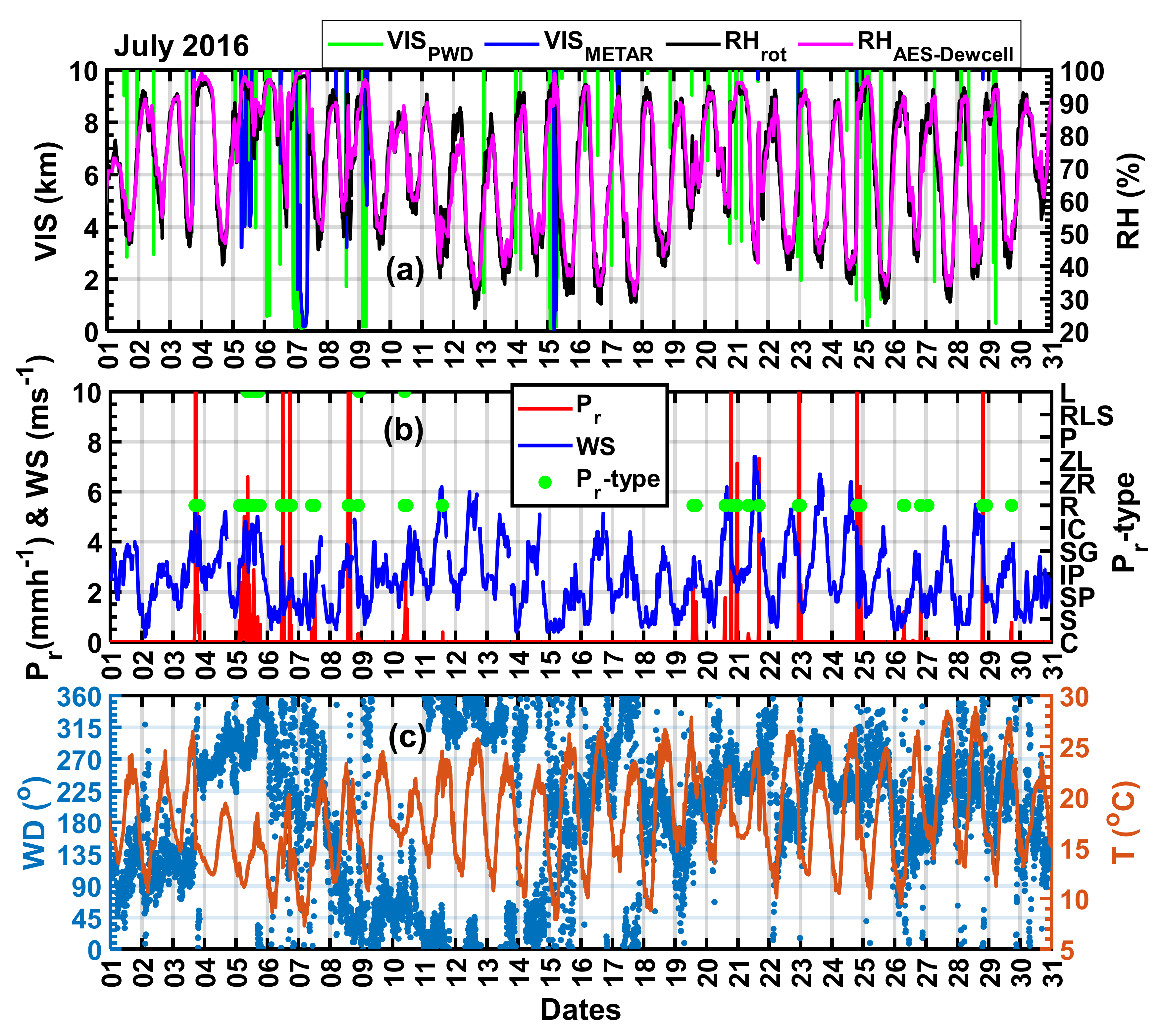
18]. The Vaisala present weather sensors identify a number of precipitation types including fog, mist or haze, snow, ice crystal, rain, drizzle, and freezing rain. If no precipitation is detected, fog is identified when the 10 min averaged visibility is less than 1 km. When the 10 min averaged visibility is between 1 km and 10 km, mist, haze or smoke conditions are identified depending on the ambient relative humidity.
During nighttime, however, when done correctly, visibility must be calculated based on a different assumption involving how far away an undirected artificial light can be seen by the human eye [
7,
19], which is usually referred to as Allard’s law [
19]. Naturally, the human eye sees a light source at night from further away than a black object during the daytime under sunny conditions [
7]. Most present weather probes, including the FS11P and PWD22, however, calculate VIS based on extinction alone during nighttime, since background light and light source intensity data are not readily available [
7]; hence, there is some ambiguity in comparing measured and METAR-based visibilities. Furthermore, these instruments also have relatively small sample volumes and are therefore not so straightforward to compare against human-based observation without ambiguity, although longer time averaging can help to compensate for this problem.
The Jenoptik model CHM15k ceilometer transmits one ns laser pulses at a wavelength of 1064 nm with a 5–7 kHz pulse repetition frequency. The backscattered signal is detected with adjustable temporal and range resolutions, which are usually set to 30 s and 15 m for an acquisition of a single vertical profile. The backscattering profile from atmospheric targets is measured over the range of 30 m to 15 km, with full overlap height of about 100 m. Using the backscattered signal information, the ceilometer calculates three cloud base heights (CBHs), as well as aerosol layers, in the planetary boundary layer using proprietary software. In this paper, the CBHs representing the first (lowest) and the second cloud layers are designated as CBH1 and CBH2, respectively. Due to the small sampling area, ceilometer data is subject to not reporting clouds not directly overhead and over-reporting clouds that linger overhead, particularly spatially limited clouds such as convective clouds with moderate to great vertical development (personal communication, Maksim Houde, a weather observer at the airport). The CBH measurements can also be affected by precipitation and hence, in this study, all precipitation cases (identified using the present weather sensors) were removed from the data.
2.3. Human Observation of Visibility and Ceiling
Human observations of VIS were made using designated visibility markers situated at different directions within a 360° view around the airdrome. These markers were viewed under sunlight during the daytime and with artificial light during the nighttime. Normally, the airdrome is divided into eight equal sectors and the prevailing VIS is determined based on the value estimated using the 5/8 portion of the airdrome and then reported in statute miles (SM) at increments of 1/8 SM, 1/4 SM, 1 SM, and 5 SM, depending on the observed visibility. For example, within the observed visibility range (3 SM < VIS < 15 SM), the prevailing VIS is reported at an increment of 1 SM (1.61 km), which is quite coarse as compared to the instruments that measure VIS in increments of 1 m. This type of reporting can be problematic in the presence of localized phenomena such as fog, which is normally reported in remarks by an observer. Therefore, it is not trivial to make definitive conclusions regarding the accuracy of the instruments for measuring VIS as compared to human observation.
According to the Manual of Surface Observation [
20] in Canada, ceiling is defined as “the height above ground or water of the base of the lowest layer of cloud where the summation amount exceeds half the sky (more than 5/10 or 4/8); or the vertical visibility in a surface-based layer that completely obscures the whole sky”. Once the ceiling is identified, the height can be determined using a hand-held or permanently installed ceilometer. At Cold Lake, a permanently installed ceilometer is used. This combined method can eliminate some of the ambiguities associated with the human guessing and ceilometer limitations mentioned earlier.
The instruments mentioned above collected data at 1 min time intervals, and the METAR data that includes the AES RH/T sensor was reported on an hourly and sub-hourly basis. For this study, combined datasets were prepared for appropriate time intervals that matched the METAR data. Although there are some uncertainties associated with both human observation and instrument measurements, it is very important to test how the instruments compare with METAR data, since they are increasingly being used autonomously for aviation applications. To minimize the uncertainty in the ceiling height and VIS comparison against human observation, the comparisons were performed only when the observer identified a ceiling that could compensate for the instrument sampling area issues mentioned earlier. The combined hourly and sub-hourly (specials) data measured and reported from January–December during the 2015–2016 period were used in this study.
4. Summary and Conclusions
Observations that were obtained using a number of commonly used ground-based in situ and remote-sensing instruments were tested against observations collected using well-established standard instruments and human-based observations. For this purpose, two years of surface observation data collected at Cold Lake, Alberta during the 2015–2016 time period was used. The specialized instruments that were tested include the Vaisala FS11P and PWD22 present weather sensors that measure horizontal visibility, the radiometric microwave radiometer (MWR) and Jenoptik CHM15k ceilometer that measure cloud base height, and the Rotronic, Vaisala WXT520, and AES-Dewcell that measure humidity (RH) and temperature (T). The main findings are given below:
Comparison of visibility measured using the Vaisala FS11P and PWD22 showed that although they are well correlated, the data exhibited significant scatter. The calculated mean difference (MD) varied from 280 m for visibility < 5 km to 490 m for visibility < 15 km under precipitation conditions, showing better agreement at lower visibilities. Generally, the FS11P measured larger visibilities compared to the PWD22. Under fog or clear conditions, the correlation between the two probes was better (R = 0.96), but the FS11P measured higher visibilities as compared to the PWD22, with a MD of 410 m and 2180 m for visibilities < 5 km and < 15 km, respectively, indicating more discrepancy between the probes under fog or clear conditions than precipitation. This analysis shows the difficulty in measuring visibility and the determination of associated uncertainties.
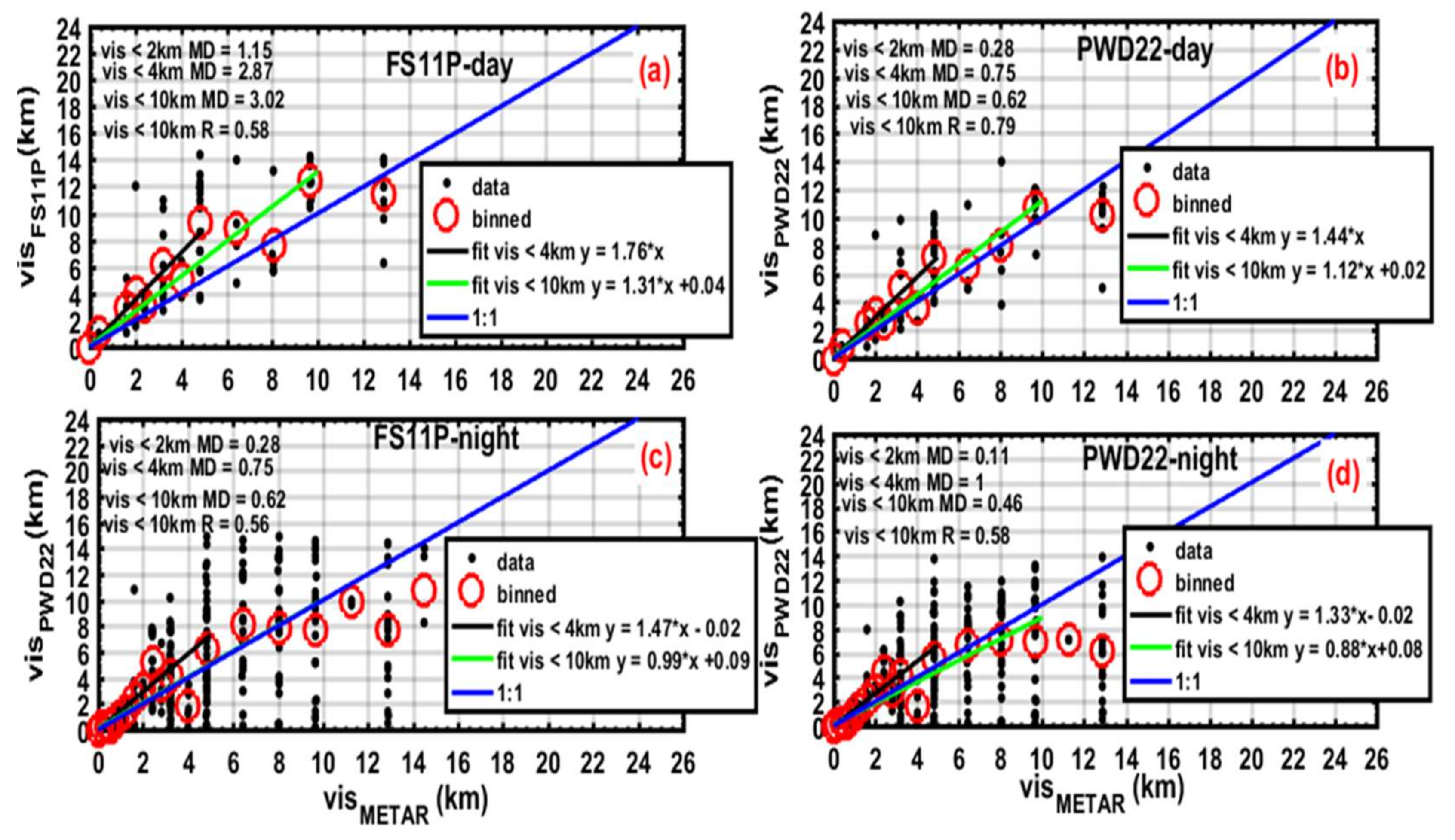
When the visibilities measured using the FS11P and PWD22 were compared against human-based observation, the data showed significant quantization, particularly at higher visibility values. This is mainly associated with limited visibility markers used by the human observer for estimating visibility. The calculated correlation coefficient for both instruments with visibility < 10 km was better than 0.6, indicating good agreement, but generally the human observer reported lower visibility values. For visibilities less than 2 km, the human observer sees on average lower visibilities, with a MD of 640 m and 370 m as compared to the FS11P and PWD22, respectively. However, for visibilities lower than 5 km, the calculated MD for the PWD22 was 0.98 km, which is better than the FS11P with a MD of almost 1.37 km, so the PWD22 probe appears to be slightly closer to human observation than the FS11P probe.
When the data was segregated based on night and day, the daytime data showed less quantization. On average, the FS11P measured higher visibilities as compared to human observation, particularly during the daytime. In contrast, the PWD22 probe measurements were close to human observation during the daytime.
Two visibility/extinction parameterizations as a function of snowfall rate were developed based on both FS11P and PWD22 measurements and the results were found to be similar, but the extinction obtained using the new coefficients reported in this study significantly underestimated the extinction parameterization obtained based on data collected in southern Ontario.
The CHM15 ceilometer on average measured lower cloud base height (CBH) compared to human observation and the calculated MDs were 390 m for CBH < 10 km and 100 m for CBH < 4 km. The correlation coefficient for the entire dataset was near 0.8, which is respectable.
The CBHs were over-estimated by the MWR for CBHs (<2 km) and under-estimated for higher CBHs. The MD between CHM15k and MWR was ≈1 km for both CBH < 4 km and CBH < 10 km, with no significant change. The CBH determined using the MWR also exhibited similar behavior when compared against human-based observations, with a relatively lower correlation of 0.65. These results suggest that CBH height determined using the method adopted in the MWR is not reliable, particularly for lower cloud base heights.
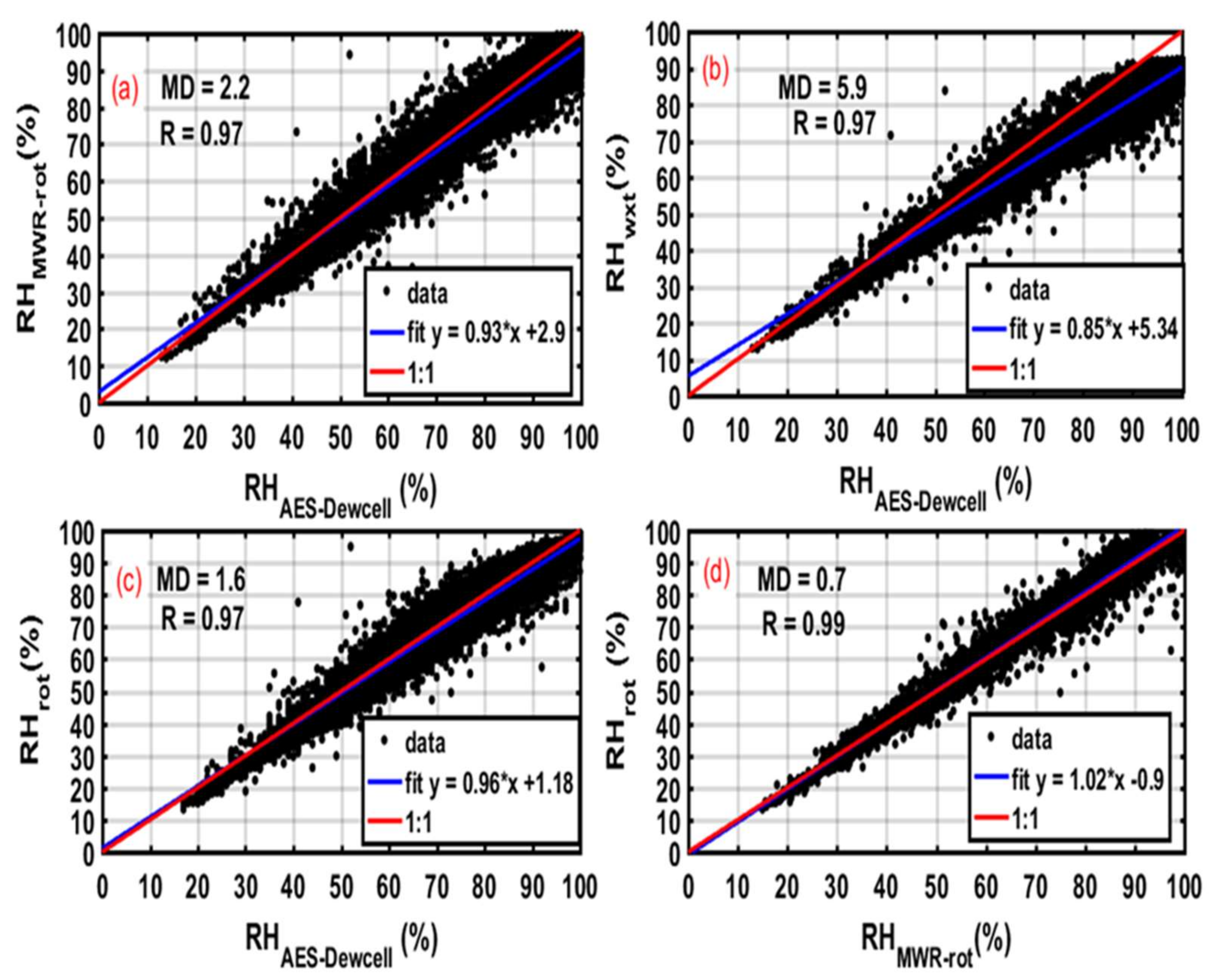
All the humidity sensors correlated well (R = 0.97) with the AES-Dewcell sensor, but all underestimated the RH, with MDs ranging from 2% for the Rotronic sensors to 6% for the WXT sensor. The uncertainty became more significant at near saturation; for example for WXT520, the error was as much as 10% at 100% RH.
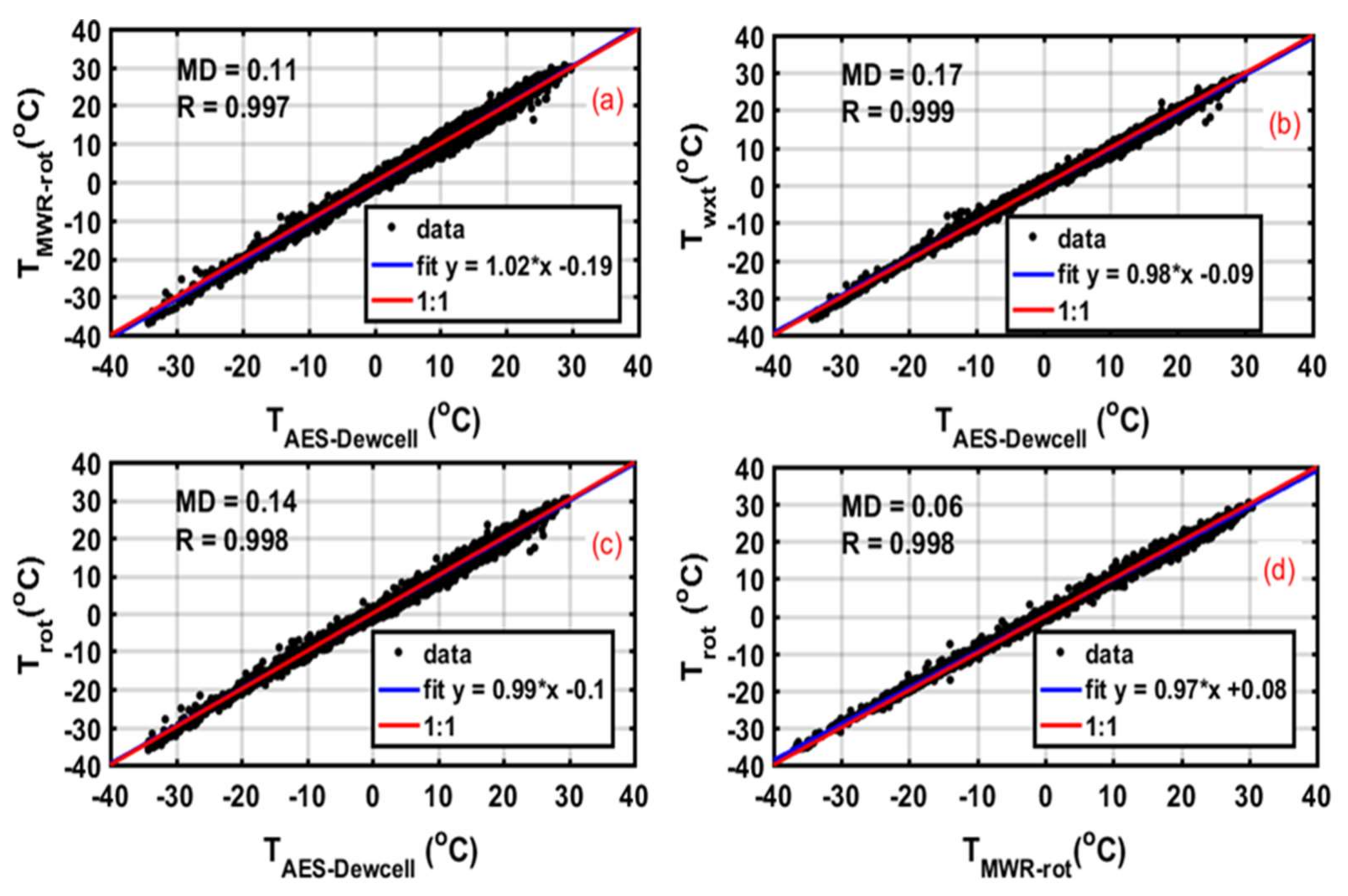
In contrast to the RH measurements, all the temperature sensors agreed quite well with a correlation coefficient (R) better than 0.99, and with an MD of less than 0.1 °C.
Based on the findings in this study, treating the data measured using the stand-alone automated meteorological instruments similar to the data obtained by human observations is potentially misleading, as it requires some corrections and adjustments before being used for model validation, aviation weather, or other applications. As shown in this study, two similar instruments do not measure precisely the same visibility, illustrating the difficulty measuring this field. The same can be said even for measuring RH, particularly close to saturation. These discrepancies could be associated with the sensitivity of a give instrument, calibration, and other factors pertaining to the location and type of weather under which the instrument is being used.


