Abstract
Lakes on the Tibet Plateau (TP) have a significant impact on the water cycle and water balance, and it is important to monitor changes in lake area and identify the influencing factors. Existing research has failed to quantitatively identify the changes and influencing factors of lakes in different regions of the TP. Thus, an eigenvector spatial filtering based spatially varying coefficient (ESF-SVC) model was used to analyze the relationship between lake area and climatic and terrain factors in the inner watershed of the TP from 2000 to 2015. A comparison with ordinary regression and spatial models showed that the ESF-SVC model eliminates spatial autocorrelation and has the best model fit and complexity. The experiments demonstrated that precipitation, snow melt, and permafrost moisture release, as well as the area of vegetation and elevation difference in the watershed, can significantly promote the expansion of lakes, while evapotranspiration and days of mean daily temperature above zero have an inhibitory effect on lake area expansion. The degree of influence of each factor also differs significantly over time and across regions. Spatially quantitative modeling of lake area in the TP using the ESF-SVC method is a new attempt to provide novel ideas for lake research.
1. Introduction
As components of the terrestrial hydrosphere, lakes participate in the natural water cycle and can, thus, reflect regional climate and environmental changes, and are indicators of climate change [1,2]. Following significant changes in the global climate, the study of the relationship between lakes and climate change has become a popular subject of research [3]. The Tibetan Plateau (TP), the “third pole” of the world, is home to the world’s highest, most numerous, and largest plateau lakes. Climate change on the TP is advanced [4], and due to its unique geographic location and special substratum, it has a significant influence on the climate of East Asia and the world [5]. Lakes on the TP are sensitive to climate change and play an important role in the natural water cycle and water balance [6]. Detecting lake areas on the TP and determining the factors that affect changes in lake areas are important in order to analyze the ecological environment of lake regions and the climate change occurring around them.
Many scholars have explored the relationship between lake areas and climatic factors on the TP using different methods. It was found that increased precipitation [7,8,9,10,11,12,13,14,15,16], higher mean temperature [8,10,11,15], melting glaciers and snow [9,10,11,12,13,16,17], permafrost moisture release [7,10,11,12], and increased runoff [8,10,13] can promote lake area expansion on the TP, whereas evapotranspiration [7,9,11,14,15] can have a suppressive effect. The main drivers of lake area change differ in different regions of the TP, and discussions of partitions have also been conducted in many studies [7,9,11,12].
The main methods for analyzing lake areas and related factors are multiple linear regression [9,11,15], structural equation modelling [14], and grey relational analysis [2,18]. Liang et al. [15] established a multiple linear regression equation and found that annual mean temperature and evapotranspiration were the main influencing factors on total lake area changes. Li et al. [14] used a structural equation model to analyze the direct and indirect effects of annual precipitation, evapotranspiration, glacier area, and mean annual temperature on lake area changes. The grey relational analysis method has been used to study the spatial response of lake changes to climate change. Yi et al. [2] classified the lakes on the TP into three grades based on the water supply conditions, and the grey relational grade of the climate series differed for different grades of lakes. However, the current analysis methods fail to consider the spatial autocorrelation and spatial heterogeneity of lake area changes. To eliminate the problem of spatial autocorrelation, an eigenvector spatial filtering (ESF) method was developed [19], which was extended to an ESF-based spatially varying coefficient (ESF-SVC) model [20]. Moreover, random effects were introduced [21] to discuss the spatial variation of the independent variables.
Previous studies mainly focused on the qualitative analysis of the effects of climate factors on lake area changes, and quantitative studies are limited. The spatial variation of lakes and the influence of different factors on lakes in different regions also need to be explored in depth. In addition, few studies have considered the influence of terrain and vegetation factors on lake area changes, and no quantitative analysis or discussion has been conducted. The vast majority of expanding lakes are located within the depressions of the TP; the local distribution of depression areas and the differences in elevation of the surrounding terrain determine the dynamic changes in the lakes [22,23]. Lake expansion depends on the average slope of the glacier end receding location, and the contraction of the glacier front edge provides the area for expansion [24]. The vegetation conditions in a watershed have a significant impact on hydrological processes, and the normalized difference vegetation index (NDVI), which uses satellite remote sensing data to describe the vegetation cover conditions in a watershed, has been widely used in hydrological simulations and other related studies [25,26,27]. Zhang pointed out that hydrological processes in lake basins are influenced by land cover, and changes in vegetation cover can cause changes in precipitation partitioning and runoff components, thus affecting lake water quantity [28].
Therefore, in this paper, an ESF-SVC model was developed to fit lake areas within different watersheds on the TP for each year from 2000 to 2015. The independent variables included evapotranspiration (EVAP), precipitation (PREC), snow melt (SME), average number of days of above-zero daily temperature per year (DAYT), land surface soil moisture (SMO), and area of vegetation cover (VAREA). In addition, the maximum elevation difference (ELEV), a terrain factor, was also included in the regressions. To quantitatively evaluate the model performance, the results of the ESF-SVC model were compared with the results of ordinary regression and spatial models based on R2, adjusted R2, pseudo-R2, RMSE, AIC, and Moran’s coefficient. The results show that the ESF-SVC model improved the goodness of fit of the regression model and could fit the relationship between each factor and the change in lake area well. On this basis, the spatial and temporal characteristics of the coefficients of independent variables and the degree of influence of different regions by each independent variable were analyzed.
2. Data and Methods
2.1. Study Area and Datasets
The TP is located in the interior of Asia, between 26°00′–39°47′N and 64°5–104°5′E, with an average elevation of up to 4000 m above sea level (masl), making it the highest plateau in the world. The lakes in this region are widely distributed and the types of water bodies are complex, which make the TP a key area for remote sensing investigation. The study area boundary data were selected from a map of river basins of the inner watershed over the TP (2016) from the National Tibetan Plateau/Third Pole Environment Data Center’s dataset [29,30], and the detailed watershed dataset within the inner watershed was obtained from the HydroSHEDS dataset [31], as shown in Figure 1. The inner TP is located between 78°–94°E and 86°–91°N, and is predominantly located within the Tibet Autonomous Region, China. The inner TP is very densely populated with lakes and has the largest overall lake area within this region and a dramatic lake area variation.
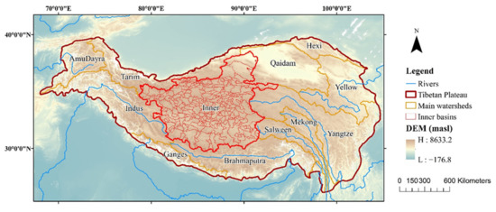
Figure 1.
Basin boundaries of TP. Twelve watersheds delineated by yellow lines are from dataset of river basins map over the TP (2016), and sub-watersheds in red are from HydroSHEDS.
The data used for water body extraction were adopted from MOD09A1 surface reflectance data [32] from 2000 to 2015. MOD09A1 is a global 500 m surface reflectance 8-day dataset that has been preprocessed. DEM data from the NASA Shuttle Radar Topography Mission (SRTM) [33,34] were used for denoising of water body and terrain factor extraction.
EVAP, PREC, and SME are the variables that have a direct effect on lake area, whereas DAYT promotes the melting of glaciers and snow on the one hand and evaporation on the other, which has an impact on the lake area. SMO is an important component of the water cycle, and changes in SMO are an important manifestation of permafrost thawing. Vegetation can cause changes in runoff components and can affect the amount of water in the lake. NDVI has been widely used in hydrological simulations and other related studies as a variable describing the vegetation cover conditions. EVAP, PREC, DAYT, and SMO were selected from a monthly mean evapotranspiration dataset for the Tibet Plateau [35,36], 1 km monthly precipitation dataset for China [37,38,39,40,41], TRIMS LST-TP [42,43,44,45], and SMsmapTE [46,47,48] from 2000–2015, respectively. Among them, EVAP is not available for 2000 and SMO is not available for 2001. SME was selected from the GLDAS_NOAH025_M dataset [49] from 2000 to 2015. NDVI data were obtained from MOD13A3 [50] from 2000 to 2015. MOD13A3 data are provided every month at a spatial resolution of 1 km. Meanwhile, DEM data were also used to extract terrain variables. Some details of the original datasets used in the experiment are provided in Table 1.

Table 1.
Details of original datasets.
2.2. Methodology
The methodology used in this study involved four steps: (1) extracting the water bodies of the TP and obtaining the yearly water body ranges from 2000 to 2015 based on terrain and time series denoising; (2) preprocessing the climate data and extracting the terrain variables; (3) constructing the spatial weight matrix, extracting the eigenvectors, and filtering the variables used in the model to construct the ESF-SVC model; and (4) selecting variables and comparing the performance of the ESF-SVC model with that of conventional non-spatial and spatial models. The stages of the research procedure are shown in Figure 2.
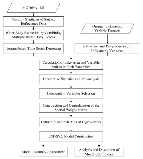
Figure 2.
Flowchart of the stages of the research procedure.
2.2.1. Yearly Lake Area Extraction
The method of extracting the lake extent of the TP was based on Che [51]. The lake areas within each watershed for each year from 2000 to 2015 were counted by monthly synthesis of surface reflectance data, water body extraction by combining multiple water body indices, and terrain-based time series denoising.
After the preprocessing work of image mosaicking, clipping, and reprojection, the MOD09A1 data were subjected to the monthly synthesis process of minimum red synthesis; that is, for all images of the current month, the pixel values in the green, near-infrared (NIR), and short-wave infrared (SWIR) bands corresponding to the smallest pixel value in the red band of each image element were selected for subsequent calculations.
The model used for water body extraction was constructed using the NDWI [52] and MNDWI [53], as shown in Formulas (1) and (2), and the synthesis of the interspectral relationship between the NIR and SWIR bands, where , , and correspond to the surface reflectance values in the B2, B4, and B6 bands of MODIS images, respectively. The detailed lake extraction process is shown in Figure 3.
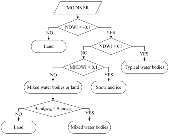
Figure 3.
Flowchart of lake detection based on multiple water indices.
After filtering the fine noise using a 5 × 5 active window, the classified images were overlaid with DEM data, and 5° was chosen as the slope threshold to filter these images, so as to eliminate misclassification caused by shadows of mountains. The water body images from May to September of each year were overlaid to discriminate, and if the probability of a pixel being identified as a water body pixel was greater than or equal to 60%, the pixel was identified as a water body pixel, thus providing an image of the yearly lake extent in the TP.
The lake area of the inner TP in 2000 is shown in Figure 4. The values of the lake areas within each watershed were calculated as dependent variables for subsequent experiments.
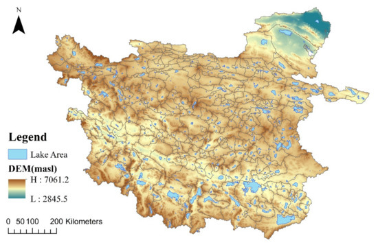
Figure 4.
Lakes within inner TP in 2000.
2.2.2. Extraction and Processing of Influencing Factors
The variables of climatic factors were preprocessed with unit conversion and annual synthesis, and the variables of terrain factors were extracted using DEM data. All variables were standardized using the scale function of R language.
The monthly raster dataset was processed for annual synthesis. The average annual values of EVAP, PREC, SME, and SMO were calculated for each raster cell after unit conversion. The average of all yearly climatic factors for each watershed between the study years was used as the independent variable. Considering that low temperatures have little effect on snow and ice melt and evapotranspiration, the average number of days of above-zero daily temperature per year (DAYT) within each basin was counted based on the daily average temperature. The annual average NDVI values were synthesized after removing the missing values of MOD13A3, and the raster with NDVI values less than 0.1 was considered to comprise non-vegetation cover pixels, which were not taken into account [54]. The area of vegetation cover (VAREA) in each watershed per year was counted. The maximum elevation difference (ELEV) within each watershed was calculated using DEM data. The preprocessed datasets were loaded in ArcMap software, as shown in Figure 5.
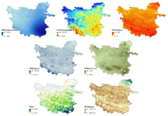
Figure 5.
Data after preprocessing (PREC, EVAP, DAYT, SME, SMO, and NDVI are yearly values in 2003).
2.2.3. Construction of ESF-based Spatially Varying Coefficient Structure
The ESF-SVC model used for lake area estimation within the inner TP can be summarized in the following five steps:
- (1)
- The first step is to construct the spatial weight matrix based on the spatial relationships of each small watershed delineated in the HydroSHEDS dataset. If two watersheds share one or more boundary point, the corresponding value in the spatial weight matrix is 1; if not, the value is 0. The spatial weight matrix was constructed using the spdep package in R language.
- (2)
- Centralize the spatial weight matrix using the following method [55]:
- (3)
- Extract eigenvectors and perform preliminary screening. The spatial weight matrix is eigen-decomposed using linear variation, the eigenvalues and eigenvectors are calculated using the “spmoran” package in R language, and the eigenvectors are initially filtered using a threshold of 0.25 [56]; thus, the filtered eigenvectors correspond to eigenvalues equal to or greater than one-fourth of the largest eigenvalue.
- (4)
- Select the appropriate eigenvectors to be used in the model. ESF-SVC regression uses a set of eigenvectors as new variables. The model introduces two new parameters α, [21], and the eigenvectors that contribute more to the regression are selected by the method of great likelihood estimation from the centralized spatial weight matrix C in the previous step and added to the model as independent variables [55]. However, the introduction of the two new parameters leads to increased complexity of the ESF-SVC model.
- (5)
- Construct the ESF-SVC model. The ESF-SVC model is built on the basis of the ESF model. In the ESF model, the eigenvectors are added to the model as follows:
Griffith [20] extended ESF to the following ESF-based SVC model, and Murakami et al. [21] showed that the random effects version of eigenvector spatial filtering regression increases the model’s accuracy with shorter computational time:
where is an vector of independent variable ; is an vector of the th independent variable; is the th EV, which is combined with its independent variable ; are the regression coefficients; represents disturbances; and denotes the element-wise product operator.
2.2.4. Variable Selection and Model Validation
The relationship between the lake area of the inner TP and climatic and terrain factors for 16 years, from 2000–2015, is discussed in this study. For each year’s experiment, the coefficients and results were analyzed by fitting the area of the lakes within each watershed with the values of the annual variables for that year.
Before conducting regression analysis, variable selection should be performed. The relationship between each variable and the lake area were examined, and the nonlinear relationship was not significant and the linear relationship dominated. Pearson correlation analysis was used to analyze the degree of linear correlation between variables, which is a classic and commonly used method, the Pearson correlation coefficient r [57] is defined in Formula (6). In previous studies, the level of significance was usually taken at 5%. When the p-value was less than 0.05, the null hypothesis should be rejected and we should be 95% certain the results are probable [58,59]. Therefore, if the p-value of Pearson’s correlation coefficient was greater than 0.05, the variable was excluded because of the uncertain reliability of the results. For those variables that were significant, if the absolute value of Pearson correlation coefficient is greater than 0.1, a certain relationship is considered to exist [60,61,62], and the independent variable can be included in the regression:
where and are the values of each variable and the lake area, respectively, and and are the average values.
In the meantime, collinearities among independent variables may lead to distortions in model estimation. The variance inflation factor (VIF) is used to measure the linear correlation between the influencing factors, which can be calculated using the vif function in the car R package, defined as:
where is the negative correlation coefficient of the independent variable on the remaining independent variables for regression analysis. If VIF > 10, severe multi-collinearity between variables is considered to exist and some variables with large VIF values need to be removed. All variables passed the multi-collinearity test for each year and were included in the regression.
An ordinary least squares (OLS) regression model, geographically weighted regression (GWR) model, spatial error model (SEM), spatial lag model (SLM), and eigenvector spatial filtering (ESF) model were chosen for comparison with the ESF-SVC model. For experiments in the specific periods, all models used the same climate and terrain variables. All models were calculated in R software. The OLS model was built using the lm function. The GWR model used the bw.gwr function in the “GWmodel” package to calculate the bandwidth and the gwr.basic function to build the model. Different kernel functions have different bandwidth sensitivities, and changes in bandwidth have a large impact on the results [63,64,65]. To reduce the error caused by inappropriate bandwidth, we employed the technique of cross-validation (CV) optimization [64,66], and chose the bisquare kernel to calculate the bandwidth of the GWR model [63,64,67]. The SEM and SLM models were constructed using the spautolm and lagsarlm functions of the “spatialreg” package, respectively, while the ESF and ESF-SVC models used the esf and resf_vc functions of the “spmoran” package.
Reliability was evaluated by performance criteria, including R2, adjusted R2, pseudo-R2, RMSE, AIC, and the global Moran coefficient of residuals (RMC). R2 represents the ratio of the dependent variable fitted from the model and can be computed from Formula (8):
where is the actual lake area, is the estimated value, and is the average value.
The adjusted R2 takes the increase into account by adding additional explanatory variables, as defined in Formula (9):
where is the number of samples and is the number of independent variables. Both R2 and adjusted R2 were used to assess the goodness of fit of the regression models. SEM and SLM do not have R2 or adjusted R2, and use pseudo-R2 to represent the goodness of fit. The closer the value of these three indicators to 1, the better the model accuracy.
Root mean square error (RMSE) measures the deviation between the observed and true values of the dependent variable and is shown in Formula (10):
where is the number of samples, is the actual lake area, and is the estimated value.
AIC is also used to estimate the relative information loss of the regression model, and is computed with Formula (11) (the smaller the AIC value, the better the model represents the relative information loss):
where is the number of independent variables, is the number of samples, is the actual lake area, and is the estimated value.
The Moran coefficient of residuals (RMC) can detect the presence of spatial autocorrelation in the residuals and determine whether the model is better able to filter spatial autocorrelation. The closer the absolute value of RMC to 0, the lower the spatial autocorrelation. RMC is calculated as shown in Formula (12):
where is the residual vector and is the spatial weight matrix.
3. Results
3.1. Pre-Analysis of Lake Area and Variables
From 2000 to 2015, the lakes in the inner TP experienced a trend of rapid growth, which was followed by slow growth. The total area of lakes increased by 5868.53 km2, with an average growth rate of 358.67 km2/y. The annual total area of lakes is shown in Figure 6.
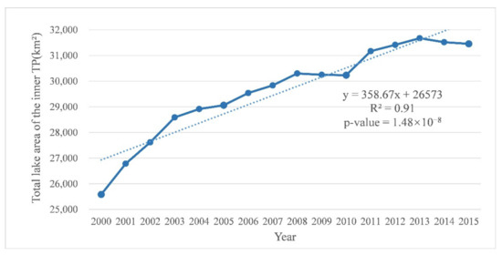
Figure 6.
Total lake area of the inner TP from 2000 to 2015.
The lake area maintained a more dramatic growth trend from 2000 to 2008, with a growth rate of about 538.78 km2/y. Then, 2008 to 2010 showed little change or even a decrease in lake area, followed by continued expansion from 2010 to 2013, but at a slower rate of about 457.56 km2/y. However, a decrease in lake area occurred in 2013 to 2015.
The lakes in the inner TP experienced different growth rates within different regions. The lake area changes and change rate within each watershed from 2000 to 2015 are shown in Figure 7. It can be seen in Figure 7A that the spatial pattern of the lake area change trend shows a southwest–northeast transition from contraction to slight expansion to rapid expansion during that time [7]. The regions with dramatic lake area growth were concentrated in the eastern and northwestern parts of the inner TP, whereas lake expansion in the central region was more moderate, and the southern region showed both increased and decreased lake area. The regions with significant increases were consistently concentrated in the West Kunlun and Karakoram Mountains, the Kumkol Basin, the Hoh Xil region, and Siling Co and its surrounding lakes. The decrease in lake area was concentrated in the southern region of Siling Co and around Zhabuye Co. From the rate of change in lake area shown in Figure 7B, although the growth of lakes in the eastern part of the inner TP was large, the change rate was not very significant due to the original distribution of large lakes in these areas. It is worth noting that some small watersheds in the central part of the inner TP had a large change rate from 2000 to 2015, indicating that a significant expansion of small- and medium-sized lakes had occurred in these regions during these sixteen years, suggesting that we need to pay attention not only to the changes of large lakes but also to the formation and expansion of small lakes.
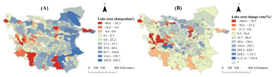
Figure 7.
Lake area changes (A) and the lake area change rate (B) in inner TP from 2000 to 2015. (* represents no lakes in the watershed in 2000).
The average values of each independent variable in all watersheds over the sixteen years were counted and preliminary analysis was performed. Table 2 shows brief descriptive statistics for each variable. As can be seen from the table, the skewness is greater than 0, indicating that the distribution of each variable is right-skewed, with the values clustered on the smaller side. The kurtosis values of SME and VAREA are large, which indicates that the data distribution of these two variables is more concentrated.
Table 2.
Descriptive statistics for each variable.
3.2. Variable Selection
Pearson correlation coefficients for each variable and lake area for each year are shown in Table 3. All variables were significantly correlated with lake area and were subjected to multi-collinearity tests between independent variables, except for EVAP and SMO, which had missing data in 2000 and 2001, respectively, and DAYT, which was not strongly correlated with lake area in 2002, 2010, 2012, and 2013.
Table 3.
Pearson correlation coefficient of each variable with lake area for each year from 2000 to 2015.
Table 4 presents the VIF values between the independent variables. The VIF values of these independent variables are less than 10 in all years, indicating that there is no significant multi-collinearity among them. Therefore, the results of the linear regression with these variables are reliable, and all variables with a certain correlation with the lake area were included in the following experiments.
Table 4.
VIF values between independent variables for each year from 2000 to 2015.
3.3. Model Accuracy Assessment
Table 5 summarizes the average model accuracy results of different models (OLS, SEM, SLM, ESF, GWR, and ESF-SVC) for the 16 years of experiments from 2000 to 2015.
Table 5.
Average results of the OLS, SEM, SLM, ESF, GWR, and ESF-SVC models from 2000 to 2015.
The average results of 16 years of experiments show that the ESF-SVC model significantly outperformed the other models in terms of R2, adjusted R2, RMSE, and AIC. In addition, the ESF-SVC model eliminated the spatial autocorrelation of the residuals, and the p-values of the Moran coefficient of residuals are all greater than 0.05. The average R2 of ESF-SVC reached 0.97, which was 28.55, 28.55, 29.23, 19.00, and 9.41% higher than that of OLS, SEM, SLM, ESF, and GWR, respectively. The ESF-SVC model also showed a very large advantage in the index of adjusted R2, which was 29.10, 20.05, and 10.91% higher than that of OLS, ESF, and GWR, respectively, and the difference with R2 was very small. In contrast, the results of ESF and GWR models showed some differences between R2 and adjusted R2. The observed values of the ESF-SVC model showed the smallest deviation from the true values, and the average RMSE was 73.72, 72.59, 71.54, 59.25, and 38.32 km² lower than that of the OLS, SEM, SLM, ESF, and GWR models, respectively. This indicates significantly higher fitting accuracy of the ESF-SVC model than the other models. The AIC values of the ESF-SVC model also remained the lowest among all experiments; the average AIC of the ESF-SVC model was 503.67, 498.51, 489.55, 405.26, and 184.96 lower than that of the OLS, SEM, SLM, ESF, and GWR models, respectively, which indicates that the ESF-SVC model not only had improved accuracy but also maintained very low complexity after adding eigenvectors and considering both spatial autocorrelation and spatial heterogeneity. From the perspective of eliminating spatial autocorrelation, the ESF-SVC model and the SEM, ESF, and GWR models can eliminate the autocorrelation of residuals, and the p-values of the Moran coefficient residuals were all greater than 0.05, whereas the OLS and SLM models exhibited the phenomenon of spatial aggregation of residuals.
The average residuals and relative errors of different models (OLS, SEM, SLM, ESF, GWR, and ESF-SVC) for the 16 years of experiments are visualized in Figure 8 and Figure 9.
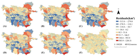
Figure 8.
Average residuals of the (A) OLS, (B) SEM, (C) SLM, (D) ESF, (E) GWR, and (F) ESF-SVC models for 2000 to 2015.
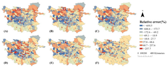
Figure 9.
Average relative errors of the (A) OLS, (B) SEM, (C) SLM, (D) ESF, (E) GWR, and (F) ESF-SVC models for 2000 to 2015.
As can be seen in Figure 8 and Figure 9, the relative and absolute residual distributions of the ESF-SVC model have no significant spatial aggregation and spatial dispersion, and the absolute and relative errors are the smallest overall.
Overall, in terms of the absolute values of the residuals, the areas with poor model fits are concentrated in the periphery of the inner TP, particularly in some watersheds in the east and south, i.e., areas with more drastic lake area changes. Instead, in terms of the relative residuals, some small watersheds in the central and western parts are fitted with poorer accuracy, which may be due to the small size of lakes in these watersheds. The results of the absolute and relative residuals have similarities with the trends of lake area changes from 2000 to 2015. This indicates that the common model cannot better explain the causes of lake area changes in each region, and also that lakes in different regions are affected by various factors to different degrees. Compared with other models, the relative and absolute residual distributions of the ESF-SVC model have no obvious spatial aggregation or spatial dispersion, and the model can eliminate the spatial autocorrelation of residuals, whereas the residual values of each region are closer to 0, which indicates that the deviation between predicted and real values is smaller. However, even with the ESF-SVC model, the predictions of lake area changes in some areas are still not accurate, probably due to the influence of some factors that were not included in the regression.
In conclusion, the ESF-SVC model proposed in this study was used to fit spatial differences in the lake area within the TP by considering spatial heterogeneity and spatial autocorrelation. The ESF-SVC model performs well in terms of eliminating spatial autocorrelation and is on par with other spatial models. In terms of fitting accuracy, model error, and model complexity, the ESF-SVC model significantly outperforms the other regression models. ESF-SVC demonstrates its excellence in all aspects of the model.
3.4. ESF-SVC Model Coefficients
The average coefficients of each variable for each year from 2000–2015 and for all experiments over the 16 years are shown in Table 6. From the average results of 16 years, lake areas showed significant positive correlations with PREC, SME, SMO, VAREA, and ELEV, and negative correlations with EVAP and DAYT. The coefficients of each variable changed from 2000 to 2015, which implies that the main influencing factors of lake expansion may have differed in different time periods. SME, SMO, VAREA, and ELEV maintained positive coefficients in all experiments, PREC had positive coefficients in most years and negative coefficients in some years, but the absolute values of the negative coefficients were small, and EVAP and DAYT had negative coefficients in most years. The coefficients of PREC were generally more dramatic, mostly positive and with larger values from 2000 to 2008, and more unstable from 2009 to 2015, with small absolute values and negative values. In contrast, the coefficients of SMO were smaller in 2000 to 2008 and larger in 2008 to 2015.
Table 6.
Average coefficients of the ESF-SVC model.
The coefficients of some independent variables in the ESF-SVC model varied spatially, and the model coefficients differed within different watersheds. The average coefficients of each region in all experiments over the 16 years were counted, as shown in Figure 10, and the spatial variation of the coefficients of the variables was analyzed.
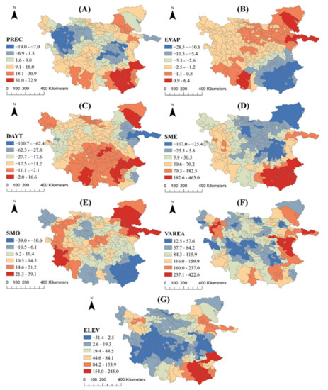
Figure 10.
Average coefficients of (A) PREC, (B) EVAP, (C) DAYT, (D) SME, (E) SMO, (F) VAREA, and (G) ELEV in the ESF-SVC model for each region from 2000 to 2015.
The average results of each coefficient in different regions for 16 years show that PREC has positive coefficients in the south and northeast, and the absolute value of the coefficient is large; however, PREC has negative coefficients in the northwest and east-central regions. EVAP shows negative coefficients in most places in the region, especially in the southeast, where the absolute value of the negative coefficient is large, while this value is small in the northeast and southwest and there are even positive coefficients. For DAYT, the negative coefficients are smaller in absolute value in the south, northwest, and northeast. The coefficient of SME is very large in the southeast, and positive coefficients are found in the western, southern, and eastern periphery, but there are also negative coefficients in the northern and central parts. For SMO, the positive coefficients are larger in the northeast and west, and for most of the central region, the coefficients are also positive, with negative coefficients existing only in the northwest and southeast. For VAREA, the distribution of coefficients is not very regular, although the coefficients are all positive, but in general, they are larger in the external parts and smaller in the internal parts. For ELEV, the coefficients are mostly negative in the central part and the positive coefficient values are larger in the external part, especially in the southeast.
The experimental results of the spatially varying coefficients show that changes in the inner TP lake area in different regions are affected by climate and terrain factors to different degrees. There are also spatial differences in the effects of each factor on lakes.
4. Discussion
4.1. Analysis of Influencing Factors
Analyzing the average results of the 16-year ESF-SVC model, it can be seen that precipitation, snow melt, permafrost moisture release, the area of vegetation in the watershed, and elevation difference all contribute significantly to lake area expansion, while evapotranspiration and days of mean daily temperature above zero have an inhibitory effect. Precipitation, snow melt, and permafrost moisture release can provide runoff to lakes and contribute directly to lake expansion [10,11,12]. Hydrological processes in lake basins are influenced by land vegetation, and changes in vegetation can cause changes in precipitation partitioning and runoff components, which can affect lake expansion [28]. Large differences in elevation in the watershed are conducive to the collection of water, and thus, the formation of small lakes [22,23]. Evapotranspiration can have a direct impact on lake area and can also reduce surface flow into lakes, negatively impacting lake expansion [9]. Temperature can promote glacier [12,68] and snow melt [12,69] on the one hand and evapotranspiration [12] on the other; thus, there is uncertainty of the effect on lake areas. The effect of temperature on snow is intuitively reflected by the SMO variable, while the contribution of temperature to glacier melt cannot be discussed quantitatively in this paper due to a lack of large-scale glacier data. The results show a negative correlation between the number of days of above-zero mean daily temperature and lake area, which may be due to the fact that most of the glaciers are distributed in the boundary area of the TP, with fewer glaciers in the inner TP [70], and the temperature has more influence on lake evapotranspiration in the inner TP.
There are fluctuations in the mean values of each coefficient across the region over the 16 years, which implies that there are differences in the degree of contribution of each variable to lake expansion at different times. These factors, such as snow melt, permafrost moisture release, vegetation area in the watershed, and elevation differences, positively influenced lake expansion from beginning to end, with precipitation contributing significantly in most years and less in some years. Evapotranspiration and days of mean daily temperature above zero inhibited lake expansion in most years. Comparing the whole period from 2000 to 2015, the inhibition of lake expansion by evapotranspiration was more pronounced from 2000 to 2008, while precipitation significantly contributed to lake expansion during the same period. The experimental results point out that the lake area maintained a faster growth rate during this period even under strong evapotranspiration, indicating that the contribution of precipitation was larger during this period compared to the subsequent period. In the period 2008 to 2015, the effects of evapotranspiration and precipitation weakened compared to the previous period, but the effects of permafrost moisture release and vegetation area in the basin increased significantly. The expansion of lakes slowed down from 2008 to 2015 compared to the previous period, and there was even shrinkage. The expansion of lakes in this period was mainly due to the moisture release of permafrost and the reduction of evapotranspiration, and the promotion of lakes by precipitation was weaker than in the previous period, which may be the reason for the slower growth rate in this period.
The differences in the spatial distribution of the coefficients of the ESF-SVC model suggest that there are differences in the effects of the factors on the lake area in different regions.
Precipitation is very effective in promoting lake expansion in the south and northeast, similar to the spatial distribution of precipitation, which is higher in the southeast of the inner TP, and these significantly contribute to the growth of lakes. In contrast, in the central and western regions, there is less precipitation and it also contributes less to the lake area compared to other regions. Evapotranspiration has a significant inhibitory effect on lake expansion in the southeastern part of the inner TP, which is similar to the distribution of evapotranspiration. The coefficient of the average days with daily temperature above zero shows that temperature inhibits the expansion of lakes within the inner TP. Above-zero temperature can promote snow and glacier melt, leading to an increase in lake area, while evapotranspiration leads to a decrease in lake area. Snow melt was added to the regression as a variable to visualize its effect on lakes, while glacier data cannot be added to the regression as a variable due to the lack of large-scale glacier data. It is hypothesized that temperature promotes more evapotranspiration due to less glacier distribution within the inner TP. However, referring to the previous classification of recharge sources of lakes on the Tibetan Plateau [71,72], the absolute value of negative coefficients in the basins where glacial lakes are located is small. Positive coefficients exist for some large glacial lake basins, suggesting that temperature does promote the expansion of glacial lakes, but the effect of evapotranspiration results in mostly negative temperature coefficients. The coefficients of snow melt show that it contributes significantly to lake expansion in most areas within the inner TP, with a particularly significant contribution in the southeast. Permafrost moisture release has a positive effect on the growth of lakes in most areas of the inner TP, which can significantly promote the expansion of lakes in the northeast. Previous studies have shown that there is some permafrost in the northeastern part of the inner TP, and the increase in soil temperature in recent years has led to a partial release of soil moisture [7], which has significantly increased in this region and promoted lake expansion. In contrast, there is only sporadically distributed permafrost in the southern part of the inner TP, and permafrost moisture release in this area has had little effect on lake expansion [7]. Vegetation in the watershed has a more pronounced effect on the lakes in the periphery of the inner TP, while it has less impact on the expansion of lakes in the central region. Since 2000, the central region of the inner TP has shown a significant trend of vegetation degradation, while the northeastern and southern regions have shown slight improvement [73,74]. Elevation differences can significantly promote lake catchment within the southeastern watersheds, while they have little effect on lake expansion within the central watersheds, probably because the watersheds in these regions are more fine-grained and have fewer elevation differences, which means less contribution to runoff convergence.
An analysis of different regions of the inner TP showed that the lake area in the northeastern part, in the Hoh Xil region, especially near the Kumkol basin, is strongly influenced by the permafrost moisture release, precipitation, evapotranspiration, temperature, and vegetation in the watershed. Measures such as active afforestation can be taken to promote lake expansion in the area. For the southeast of the inner TP, south of the Tanggula Mountains and north of the Nyainqentanglha Mountains, the influence of precipitation and snow melt on lake expansion is dominant, while the elevation difference within the basin also promotes lake water collection. Meanwhile, the influence of evapotranspiration is also strong in the region, but the significant expansion of lakes in recent years indicates that the promotion of precipitation, snow melt, and other runoff is higher than the inhibition of evapotranspiration, and some glacial lake basins in the region also show a positive correlation with higher temperature.
4.2. Limitations and Future Enhancement
Although the ESF-SVC model achieved higher accuracy, it also has some limitations. In the ESF and ESF-SVC models, a reliable spatial weight matrix can improve the fitting accuracy and prediction ability. This is similar to the use of a spatial weight matrix and bandwidth selection to express spatial correlation in the GWR model, in which CV optimization is used to select the appropriate bandwidth. However, neither the ESF nor the ESF-SVC model uses this technique. Another shortcoming of this experiment is that some factors that have an impact on lake area, such as glacier data, were not included in the regression, mainly due to a lack of data. In addition, the resolution of data collected in this paper, such as snow melt and soil moisture, is too coarse, so the climate values of adjacent small watersheds may be similar; thus, these data cannot accurately reflect the impact of spatial variations in climate on the TP, and cannot improve the modelling of lake area. Additionally, the approach in this manuscript explores the linear relationship between lake area and related factors, but the discussion of the nonlinear relationship is lacking. Subsequently, we can explore how to add the effects of nonlinearity into the regression for analysis. In addition, there are differences in the influencing factors and the degree of influence on glacier-fed and non-glacier-fed lakes. This study uses the watershed as the study unit, and it may not be possible to discuss in depth the differences in the drivers of expansion of lakes with different supply sources. In a subsequent study, we can distinguish different supply sources of lakes and discuss their influencing factors separately. The effect of human activities on lake areas in regressions in subsequent experiments should also be considered.
5. Conclusions
The changes in lake areas within the inner TP from 2000 to 2015 were explored, and the effects of climate, terrain factors, and spatial effects were discussed. Using the ESF-SVC model, a regression analysis of lake area in the inner TP was conducted during the 16 years, using data on evapotranspiration, precipitation, snow melt, days of above-zero daily temperature, land surface soil moisture, vegetation zone area, and maximum elevation difference within the watershed.
The results show that the ESF-SVC model had the best fit in all experiments during the 16 years and had the best performance according to R2, adjusted R2, pseudo-R2, RMSE, and AIC criteria and was able to eliminate spatial autocorrelation. The advantage of the method in our paper compared with previous studies is the ability to quantitatively analyze the effects of multiple factors on lake areas in different spatial regions. Compared with other spatial and non-spatial models, the ESF-SVC model took better account of spatial autocorrelation and spatial heterogeneity by incorporating the eigenvectors selected from the spatial weight matrix into the regression, which not only improved the accuracy and reduced the fitting error, but also maintained a very low complexity. In addition, the model results showed spatial differences in the degree of influence of each factor, thus allowing us to explore the differences in the drivers of lake expansion in different regions.
The average coefficients of the ESF-SVC model over the 16 years show that precipitation, snow melt, permafrost moisture release, the area of vegetation, and elevation difference in the watershed contribute significantly to lake area expansion, while evapotranspiration and days of mean daily temperature above zero have an inhibitory effect. The values of the coefficients of each variable fluctuate somewhat in different years, which means that the degree of contribution of each variable to lake expansion varies at different times. At the same time, differences in the spatial distribution of the mean coefficients of each variable in the 16 years indicate that there are differences in the effects of each factor on the lake area in different regions. In conclusion, the factors influencing the lakes of the TP at different times and in different regions are not consistent.
In this study, a quantitative spatial modeling of lake area on TP was conducted. This work represents a new attempt to study lakes on the TP, exploring the differences in influencing factors of lakes from temporal and spatial scales, and including factors of vegetation and terrain into the discussion for subsequent studies of lakes, which provides a reference for subsequent spatial studies of lake areas on TP. Compared with traditional spatial models, the ESF-SVC model provides a suitable approach for analyzing geographic events and a unique perspective. However, there is no more universal method for the ESF-SVC model to construct the spatial weight matrix yet, which may have a significant impact on the results, and further discussion may be needed. It is foreseen that the proposed model is a highly promising approach for application in spatial regression modeling.
Author Contributions
Z.X.: Conceptualization, Methodology, Software, Writing—original draft preparation. Y.C.: Conceptualization, Supervision. H.T.: Methodology, Software. Q.C.: Data curation, Validation. A.Z.: Validation, Visualization. All authors have read and agreed to the published version of the manuscript.
Funding
This study was supported by the National Key Research and Development Program of China [Grant No. 2017YFB0503704].
Institutional Review Board Statement
Not applicable.
Informed Consent Statement
Not applicable.
Data Availability Statement
Not applicable.
Acknowledgments
We would like to acknowledge the National Tibetan Plateau/Third Pole Environment Data Center, the U.S. National Aeronautics and Space Administration (NASA) and HydroSHEDS for providing datasets.
Conflicts of Interest
The authors declare no conflict of interest.
References
- Yan, L.; Zheng, M.; Wei, L. Change of the lakes in Tibetan Plateau and its response to climate in the past forty years. Earth Sci. Front. 2016, 23, 310–323. [Google Scholar]
- Yi, G.-H.; Deng, W.; Li, A.-N.; Zhang, T.-B. Response of lakes to climate change in Xainza basin Tibetan Plateau using multi-mission satellite data from 1976 to 2008. J. Mt. Sci. 2015, 12, 604–613. [Google Scholar] [CrossRef]
- Oviatt, C.G. Lake Bonneville fluctuations and global climate change. Geology 1997, 25, 155–158. [Google Scholar] [CrossRef]
- Yao, T.D.; Xie, Z.C.; Wu, X.L.; Thompson, L.G. Climatic-Change Since Little Ice-Age Recorded by Dunde Ice Cap. Sci. China Ser. B-Chem. Life Sci. Earth Sci. 1991, 34, 760–767. [Google Scholar]
- Yanai, M.H.; Li, C.F.; Song, Z.S. Seasonal Heating of the Tibetan Plateau and Its Effects on the Evolution of the Asian Summer Monsoon. J. Meteorol. Soc. Jpn. 1992, 70, 319–351. [Google Scholar] [CrossRef] [Green Version]
- Lv, L.; Zhang, T.; Yi, G.; Miao, J.; Li, J.; Bie, X.; Huang, X. Changes of lake areas and its response to the climatic factors in Tibetan Plateau since 2000. J. Lake Sci. 2019, 31, 573–589. [Google Scholar]
- Liu, W.H.; Xie, C.W.; Zhao, L.; Li, R.; Liu, G.Y.; Wang, W.; Liu, H.R.; Wu, T.H.; Yang, G.Q.; Zhang, Y.X.; et al. Rapid expansion of lakes in the endorheic basin on the Qinghai-Tibet Plateau since 2000 and its potential drivers. Catena 2021, 197, 104942. [Google Scholar] [CrossRef]
- Liu, J.; Wang, S.; Yu, S.; Yang, D.; Zhang, L. Climate warming and growth of high-elevation inland lakes on the Tibetan Plateau. Glob. Planet. Chang. 2009, 67, 209–217. [Google Scholar] [CrossRef]
- Song, C.; Huang, B.; Richards, K.; Ke, L.; Vu Hien, P. Accelerated lake expansion on the Tibetan Plateau in the 2000s: Induced by glacial melting or other processes? Water Resour. Res. 2014, 50, 3170–3186. [Google Scholar] [CrossRef] [Green Version]
- Huang, L.; Liu, J.; Shao, Q.; Liu, R. Changing inland lakes responding to climate warming in Northeastern Tibetan Plateau. Clim. Chang. 2011, 109, 479–502. [Google Scholar] [CrossRef]
- Liao, J.; Shen, G.; Li, Y. Lake variations in response to climate change in the Tibetan Plateau in the past 40 years. Int. J. Digit. Earth 2013, 6, 534–549. [Google Scholar] [CrossRef]
- Mao, D.; Wang, Z.; Yang, H.; Li, H.; Thompson, J.R.; Li, L.; Song, K.; Chen, B.; Gao, H.; Wu, J. Impacts of Climate Change on Tibetan Lakes: Patterns and Processes. Remote Sens. 2018, 10, 358. [Google Scholar] [CrossRef] [Green Version]
- Yang, X.; Lu, X.; Park, E.; Tarolli, P. Impacts of Climate Change on Lake Fluctuations in the Hindu Kush-Himalaya-Tibetan Plateau. Remote Sens. 2019, 11, 1082. [Google Scholar] [CrossRef] [Green Version]
- Li, H.; Mao, D.; Li, X.; Wang, Z.; Wang, C. Monitoring 40-Year Lake Area Changes of the Qaidam Basin, Tibetan Plateau, Using Landsat Time Series. Remote Sens. 2019, 11, 343. [Google Scholar] [CrossRef] [Green Version]
- Liang, B.; Qi, S.; Li, Z.; Li, Y.; Chen, J. Dynamic Change of Lake Area over the Tibetan Plateau and Its Response to Climate Change. Mt. Res. 2018, 36, 206–216. [Google Scholar]
- Brun, F.; Treichler, D.; Shean, D.; Immerzeel, W.W. Limited Contribution of Glacier Mass Loss to the Recent Increase in Tibetan Plateau Lake Volume. Front. Earth Sci. 2020, 8, 495. [Google Scholar] [CrossRef]
- Yao, T.; Pu, J.; Lu, A.; Wang, Y.; Yu, W. Recent glacial retreat and its impact on hydrological processes on the tibetan plateau, China, and sorrounding regions. Arct. Antarct. Alp. Res. 2007, 39, 642–650. [Google Scholar] [CrossRef] [Green Version]
- Xing, Y.; Sun, Y.; Li, W.; Li, Y.; Fu, C. Variation of lakes in Qinghai-Tibet Plateau and its spatial response to climatic change based on Grey relational analysis. J. Arid. Land Resour. Environ. 2017, 31, 158–163. [Google Scholar]
- Griffith, D.A. Spatial autocorrelation and eigenfunctions of the geographic weights matrix accompanying geo-referenced data. Can. Geogr.-Geogr. Can. 1996, 40, 351–367. [Google Scholar] [CrossRef]
- Griffith, D.A. Spatial-filtering-based contributions to a critique of geographically weighted regression (GWR). Environ. Plan. Econ. Space 2008, 40, 2751–2769. [Google Scholar] [CrossRef]
- Murakami, D.; Yoshida, T.; Seya, H.; Griffith, D.A.; Yamagata, Y. A Moran coefficient-based mixed effects approach to investigate spatially varying relationships. Spat. Stat. 2017, 19, 68–89. [Google Scholar] [CrossRef] [Green Version]
- Yu, X.; Qigang, J.; Kun, W.; Bin, C.; Yuanhua, L.I.; Gengming, W.; Honghong, Z. Production and application on DEM of Tibetan Plateau. World Geol. 2007, 26, 479–483. [Google Scholar]
- Wei, S.; Jin, X.; Wang, K.; Liang, H. Response of lake area variation to climate change in Qaidam Basin based onremote sensing. Earth Sci. Front. 2017, 24, 427–433. [Google Scholar]
- Song, C.; Sheng, Y.; Wang, J.; Ke, L.; Madson, A.; Nie, Y. Heterogeneous glacial lake changes and links of lake expansions to the rapid thinning of adjacent glacier termini in the Himalayas. Geomorphology 2017, 280, 30–38. [Google Scholar] [CrossRef] [Green Version]
- Zhang, S.; Yang, H.; Yang, D.; Jayawardena, A.W. Quantifying the effect of vegetation change on the regional water balance within the Budyko framework. Geophys. Res. Lett. 2016, 43, 1140–1148. [Google Scholar] [CrossRef]
- Xiong, L.; Liu, S.; Xiong, B.; Xu, W. Impacts of vegetation and human activities on temporal variation of the parameters in a monthly water balance model. Adv. Water Sci. 2018, 29, 625–635. [Google Scholar]
- Deng, C.; Liu, P.; Wang, D.; Wang, W. Temporal variation and scaling of parameters for a monthly hydrologic model. J. Hydrol. 2018, 558, 290–300. [Google Scholar] [CrossRef]
- Zhang, Q. Hydrology of Lake Catchment: Research Status and Challenges. Resour. Environ. Yangtze Basin 2021, 30, 1559–1573. [Google Scholar]
- Guoqing, Z. Dataset of River Basins Map over the TP (2016). 2019. Available online: https://data.tpdc.ac.cn/en/data/dff6b437-90a1-4729-8140-faafc544860f/ (accessed on 14 December 2021).
- Zhang, G.; Yao, T.; Xie, H.; Kang, S.; Lei, Y. Increased mass over the Tibetan Plateau: From lakes or glaciers? Geophys. Res. Lett. 2013, 40, 2125–2130. [Google Scholar] [CrossRef]
- Lehner, B.; Grill, G. Global river hydrography and network routing: Baseline data and new approaches to study the world’s large river systems. Hydrol. Process. 2013, 27, 2171–2186. [Google Scholar] [CrossRef]
- Vermote, E. MOD09A1 MODIS/Terra Surface Reflectance 8-Day L3 Global 500m SIN Grid V006, NASA EOSDIS Land Processes DAAC. 2015. Available online: https://lpdaac.usgs.gov/products/mod09a1v006/ (accessed on 14 December 2021).
- Reuter, H.I.; Nelson, A.; Jarvis, A. An evaluation of void-filling interpolation methods for SRTM data. Int. J. Geogr. Inf. Sci. 2007, 21, 983–1008. [Google Scholar] [CrossRef]
- Jarvis, A.H.I.R.; Nelson, A.; Guevara, E. Hole-filled Seamless SRTM Data V4, International Centre for Tropical Agriculture (CIAT). 2008. Available online: https://srtm.csi.cgiar.org (accessed on 4 November 2020).
- Han, C.; Ma, Y.; Wang, B.; Zhong, L.; Ma, W.; Chen, X.; Su, Z. Monthly mean evapotranspiration data set of the Tibet Plateau (2001–2018). Natl. Tibet. Plateau Data Cen. 2020. [Google Scholar] [CrossRef]
- Han, C.; Ma, Y.; Wang, B.; Zhong, L.; Ma, W.; Chen, X.; Su, Z. Long-term variations in actual evapotranspiration over the Tibetan Plateau. Earth Syst. Sci. Data 2021, 13, 3513–3524. [Google Scholar] [CrossRef]
- Peng, S.Z. 1-km Monthly Precipitation Dataset for China (1901–2017). 2020. Available online: https://data.tpdc.ac.cn/en/data/faae7605-a0f2-4d18-b28f-5cee413766a2/ (accessed on 14 December 2021).
- Ding, Y.; Peng, S. Spatiotemporal Trends and Attribution of Drought across China from 1901–2100. Sustainability 2020, 12, 477. [Google Scholar] [CrossRef] [Green Version]
- Peng, S.; Ding, Y.; Wen, Z.; Chen, Y.; Cao, Y.; Ren, J. Spatiotemporal change and trend analysis of potential evapotranspiration over the Loess Plateau of China during 2011–2100. Agric. For. Meteorol. 2017, 233, 183–194. [Google Scholar] [CrossRef] [Green Version]
- Peng, S.; Ding, Y.; Liu, W.; Li, Z. 1 km monthly temperature and precipitation dataset for China from 1901 to 2017. Earth Syst. Sci. Data 2019, 11, 1931–1946. [Google Scholar] [CrossRef] [Green Version]
- Peng, S.; Gang, C.; Cao, Y.; Chen, Y. Assessment of climate change trends over the Loess Plateau in China from 1901 to 2100. Int. J. Climatol. 2018, 38, 2250–2264. [Google Scholar] [CrossRef]
- Xiaodong, Z.; Ji, Z.; Wenbin, T.; Lirong, D.; Jin, M.; Xu, Z. Daily 1-km All-Weather Land Surface Temperature Dataset for Western China (TRIMS LST-TP; 2000–2020) V2. 2019. Available online: https://www.tpdc.ac.cn/en/data/76006ce7-b8dc-4add-bbb5-93f36f4bd26c/?q= (accessed on 14 December 2021).
- Zhang, X.; Zhou, J.; Liang, S.; Wang, D. A practical reanalysis data and thermal infrared remote sensing data merging (RTM) method for reconstruction of a 1-km all-weather land surface temperature. Remote. Sens. Environ. 2021, 260, 112437. [Google Scholar] [CrossRef]
- Zhang, X.; Zhou, J.; Goettsche, F.-M.; Zhan, W.; Liu, S.; Cao, R. A Method Based on Temporal Component Decomposition for Estimating 1-km All-Weather Land Surface Temperature by Merging Satellite Thermal Infrared and Passive Microwave Observations [Feb 19 4670–4691]. IEEE Trans. Geosci. Remote Sens. 2019, 57, 6254. [Google Scholar] [CrossRef]
- Zhou, J.; Zhang, X.; Zhan, W.; Goettsche, F.-M.; Liu, S.; Olesen, F.-S.; Hu, W.; Dai, F. A Thermal Sampling Depth Correction Method for Land Surface Temperature Estimation from Satellite Passive Microwave Observation Over Barren Land. Ieee Trans. Geosci. Remote Sens. 2017, 55, 4743–4756. [Google Scholar] [CrossRef]
- Linna, C.; Zhongli, Z.; Shaomin, L. Land Surface Soil Moisture Dataset of SMAP Time-Expanded Daily 0.25°×0.25° over Qinghai-Tibet Plateau Area (SMsmapTE, V1). 2020. Available online: http://60.245.210.47/en/data/9033c624-737e-4c80-9f07-29dd5386d44a/?q= (accessed on 14 December 2021).
- Qu, Y.; Zhu, Z.; Chai, L.; Liu, S.; Montzka, C.; Liu, J.; Yang, X.; Lu, Z.; Jin, R.; Li, X.; et al. Rebuilding a Microwave Soil Moisture Product Using Random Forest Adopting AMSR-E/AMSR2 Brightness Temperature and SMAP over the Qinghai-Tibet Plateau, China. Remote Sens. 2019, 11, 683. [Google Scholar] [CrossRef] [Green Version]
- Liu, J.; Chai, L.; Lu, Z.; Liu, S.; Qu, Y.; Geng, D.; Song, Y.; Guan, Y.; Guo, Z.; Wang, J.; et al. Evaluation of SMAP, SMOS-IC, FY3B, JAXA, and LPRM Soil Moisture Products over the Qinghai-Tibet Plateau and Its Surrounding Areas. Remote Sens. 2019, 11, 792. [Google Scholar] [CrossRef] [Green Version]
- Beaudoing, H.; Rodell, M. GLDAS Noah Land Surface Model L4 monthly 0.25 x 0.25 Degree V2.1; NASA/GSFC/HSL; Goddard Earth Sciences Data and Information Services Center (GES DISC): Greenbelt, MD, USA, 2020.
- Didan, K. MOD13A3 MODIS/Terra Vegetation Indices Monthly L3 Global 1 km SIN Grid V006; NASA EOSDIS Land Processes DAAC; 2015. Available online: https://lpdaac.usgs.gov/products/mod13a3v006/ (accessed on 14 December 2021).
- Che, X.; Feng, M.; Jiang, H.; Xiao, T.; Wang, C.; Jia, B.; Bai, Y. Detection and Analysis of Qinghai-Tibet Plateau Lake Area from 2000 to 2013. J. Geo-Inf. Sci. 2015, 17, 99–107. [Google Scholar]
- McFeeters, S.K. The use of the normalized difference water index (NDWI) in the delineation of open water features. Int. J. Remote Sens. 1996, 17, 1425–1432. [Google Scholar] [CrossRef]
- Xu, H.Q. Modification of normalised difference water index (NDWI) to enhance open water features in remotely sensed imagery. Int. J. Remote Sens. 2006, 27, 3025–3033. [Google Scholar] [CrossRef]
- YuanHe, Y.; ShiLong, P. Variations in Grassland Vegetation Cover in Relation to Climatic Factors on The Tibetan Plateau. Acta Phytoecol. Sin. 2006, 30, 1–8. [Google Scholar] [CrossRef]
- Griffith, D.; Chun, Y. Spatial Autocorrelation and Spatial Filtering. In Handbook of Regional Science; Fischer, M.M., Nijkamp, P., Eds.; Springer: Berlin/Heidelberg, Germany, 2014; pp. 1477–1507. [Google Scholar]
- Murakami, D.; Griffith, D.A. Random effects specifications in eigenvector spatial filtering: A simulation study. J. Geogr. Syst. 2015, 17, 311–331. [Google Scholar] [CrossRef]
- Zou, K.H.; Tuncali, K.; Silverman, S.G. Correlation and simple linear regression. Radiology 2003, 227, 617–622. [Google Scholar] [CrossRef]
- Siegel, A.F. Chapter 10—Hypothesis Testing: Deciding Between Reality and Coincidence. In Practical Business Statistics, 7th ed.; Siegel, A.F., Ed.; Academic Press: Cambridge, MA, USA, 2016; pp. 255–295. [Google Scholar]
- Loftus, S.C. The idea behind testing hypotheses. In Basic Statistics with R; Loftus, S.C., Ed.; Academic Press: Cambridge, MA, USA, 2022; Chapter 10; pp. 109–115. [Google Scholar]
- Tan, H.; Chen, Y.; Wilson, J.P.; Zhang, J.; Cao, J.; Chu, T. An eigenvector spatial filtering based spatially varying coefficient model for PM2.5 concentration estimation: A case study in Yangtze River Delta region of China. Atmos. Environ. 2020, 223, 117205. [Google Scholar] [CrossRef]
- Zongming, W.; Bai, Z.; Xiaoyan, L.I.; Dianwei, L.I.U.; Kaishan, S.; Jianping, L.I. Analyses of Affecting Factors for Spatial Distribution of Actual Crop Productivity in Songnen Plain. J. Arid. Land Resour. Environ. 2007, 21, 85–91. [Google Scholar]
- Lin, P. Urbanization Effects on Mammal Richness:A Case Study of Yangtze River Delta Urban Agglomeration. Acta Sci. Nat. Univ. Pekin. 2021, 57, 565–574. [Google Scholar]
- Gollini, I.; Lu, B.; Charlton, M.; Brunsdon, C.; Harris, P. GWmodel: An R Package for Exploring Spatial Heterogeneity Using Geographically Weighted Models. J. Stat. Softw. 2015, 63, 1–50. [Google Scholar] [CrossRef] [Green Version]
- Li, G.; Li, R.; Lu, Y.; Zhao, Y.; Yu, B. Using Principal Component Analysis and Geographic Weighted Regression Methods to Analyze AOD Data. Bull. Surv. Mapp. 2018, 4, 50–56. [Google Scholar]
- Zhao, Y.; Liu, J.; Xu, S.; Zhang, F.; Yang, Y. A Geographic Weighted Regression Method Based on Semi-supervised Learning. Acta Geod. Et Cartogr. Sin. 2017, 46, 123–129. [Google Scholar]
- Cleveland, W.S. Robust Locally Weighted Regression and Smoothing Scatterplots. J. Am. Stat. Assoc. 1979, 74, 829–836. [Google Scholar] [CrossRef]
- Fotheringham, A.S.; Charlton, M.E.; Brunsdon, C. Geographically weighted regression: A natural evolution of the expansion method for spatial data analysis. Environ. Plan. A 1998, 30, 1905–1927. [Google Scholar] [CrossRef]
- Yao, T.D.; Thompson, L.; Yang, W.; Yu, W.S.; Gao, Y.; Guo, X.J.; Yang, X.X.; Duan, K.Q.; Zhao, H.B.; Xu, B.Q.; et al. Different glacier status with atmospheric circulations in Tibetan Plateau and surroundings. Nat. Clim. Chang. 2012, 2, 663–667. [Google Scholar] [CrossRef]
- Cheng, G.D.; Wu, T.H. Responses of permafrost to climate change and their environmental significance, Qinghai-Tibet Plateau. J. Geophys. Res. -Earth Surf. 2007, 112. [Google Scholar] [CrossRef] [Green Version]
- Liu, S.; Yao, X.; Guo, W.; Xu, J.; Shangguan, D.; Wei, J.; Bao, W.; Wu, L. The contemporary glaciers in China based on the Second Chinese Glacier Inventory. Acta Geogr. Sin. 2015, 70, 3–16. [Google Scholar]
- Guoqing, Z. Lake Volume Changes on the Tibetan Plateau during 1976–2019 (>1 km2). 2021. Available online: http://60.245.210.47/en/data/f1643e88-f6e5-4924-882c-75cbd9cdea5c/?q= (accessed on 14 December 2021).
- Zhang, G.; Bolch, T.; Chen, W.; Cretaux, J.-F. Comprehensive estimation of lake volume changes on the Tibetan Plateau during 1976–2019 and basin-wide glacier contribution. Sci. Total Environ. 2021, 772, 145463. [Google Scholar] [CrossRef]
- Wang, Q.; Lu, S.; Bao, Y.; Ma, D.; Li, R. Characteristics of Vegetation Change and Its Relationship with Climate Factors in Different Time-Scales on Qinghai-Xizang Plateau. Plateau Meteorol. 2014, 33, 301–312. [Google Scholar]
- Zhao, Z. Temporal and spatial variation analysis of vegetation on the Tibetan Plateau from 1982 to 2013. Sci. Surv. Mapp. 2017, 42, 62–70. [Google Scholar]
Publisher’s Note: MDPI stays neutral with regard to jurisdictional claims in published maps and institutional affiliations. |
© 2021 by the authors. Licensee MDPI, Basel, Switzerland. This article is an open access article distributed under the terms and conditions of the Creative Commons Attribution (CC BY) license (https://creativecommons.org/licenses/by/4.0/).