
Pyramid Information Distillation Attention Network for Super-Resolution Reconstruction of Remote Sensing Images


Abstract
:
1. Introduction
- (1)
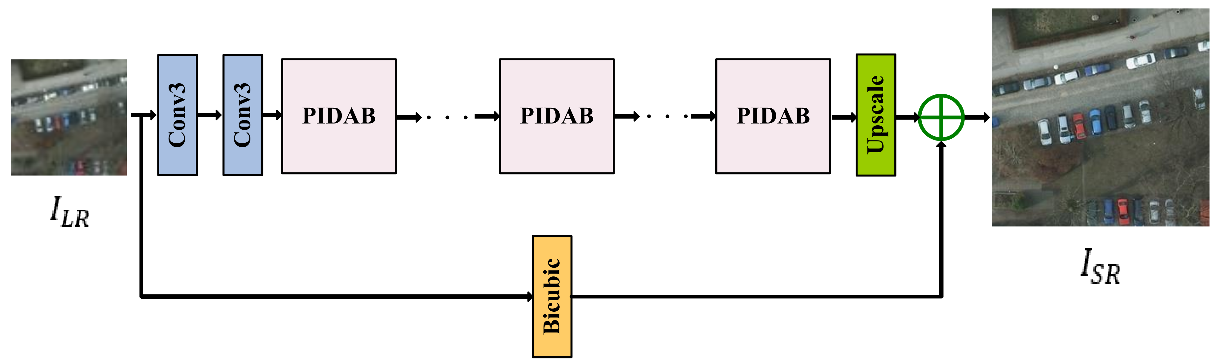
- Inspired by IDNs, we constructed an effective and convenient end-to-end trainable architecture, PIDAN, which is designed for SR reconstruction of remote sensing images. Our PIDAN structure consists of a shallow feature-extraction part, stacked PIDABs, and a reconstruction part. Compared with an IDN, a PIDAN recovers more high-frequency information.
- (2)
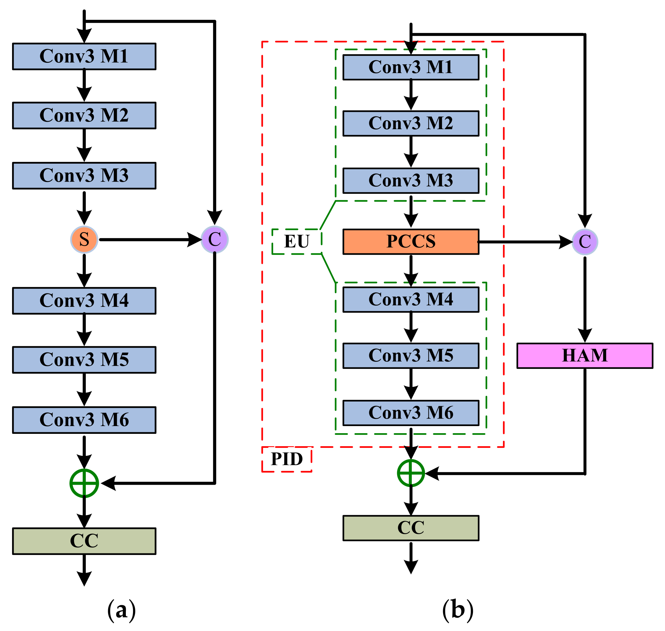
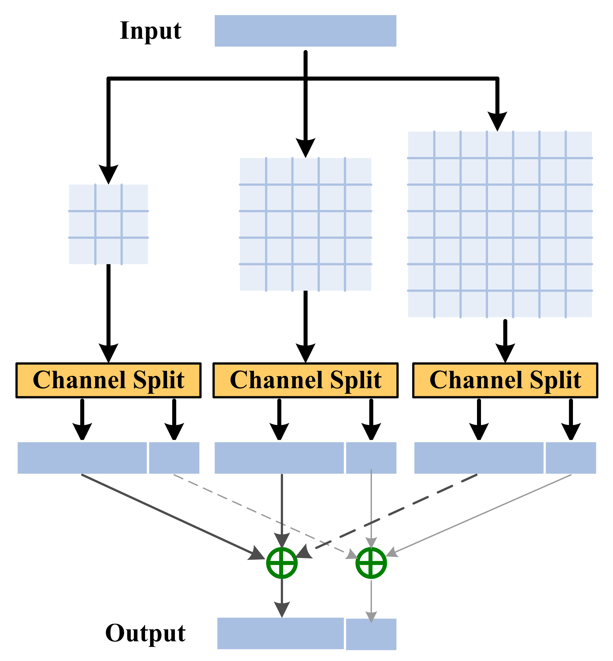
- Specifically, we propose the PIDAB, which is composed of a PID module, a HAM module, and a single CC unit. Firstly, the PID module uses an EU and a PCCS operation to gradually integrate the local short- and long-path features for reconstruction. Secondly, the HAM utilizes the short-path feature information by fusing a CAM and SAM in parallel. Finally, the CC unit is used for achieving channel dimensionality reduction.
- (3)
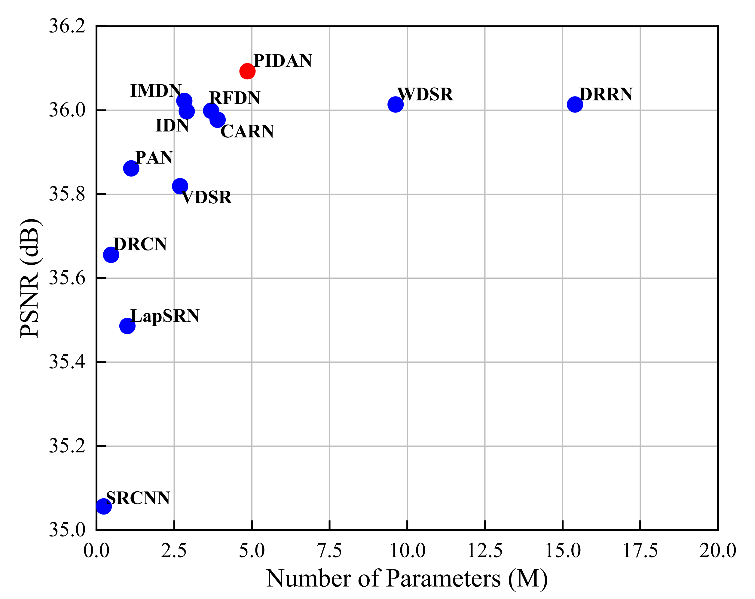
- We compared our PIDAN with other advanced SISR approaches using remote sensing datasets. The extensive experimental results demonstrate that the PIDAN achieves a better balance between SR performance and model complexity than the other approaches.
2. Related Works
2.1. CNN-Based SR Methods
2.2. Attention Mechanisms
3. Methodology
3.1. Network Architecture
3.2. PIDAB
3.2.1. PID Module
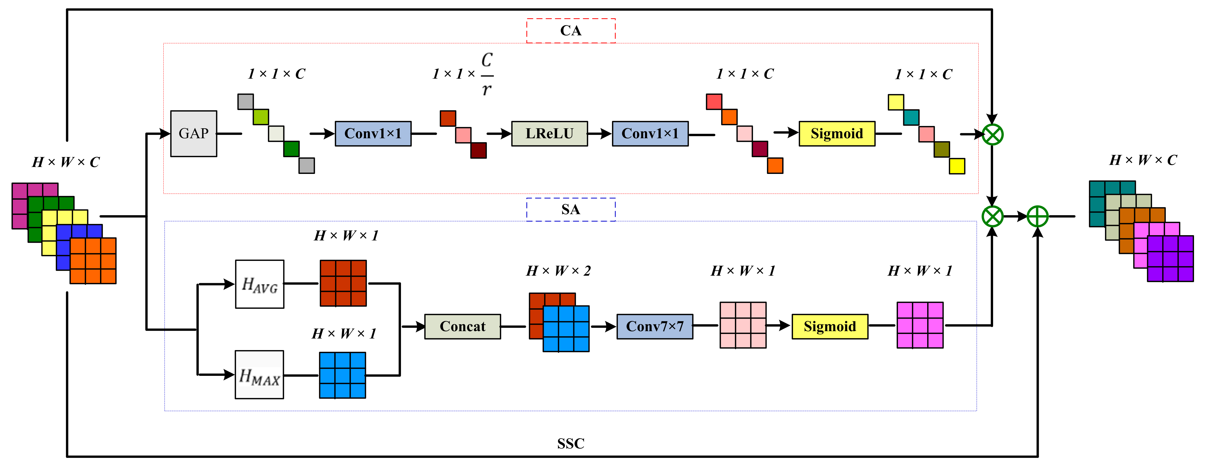
3.2.2. HAM Module
Channel Attention Mechanism
Spatial Attention Mechanism
3.2.3. CC Unit
3.3. Loss Function
4. Experiments and Results
4.1. Settings
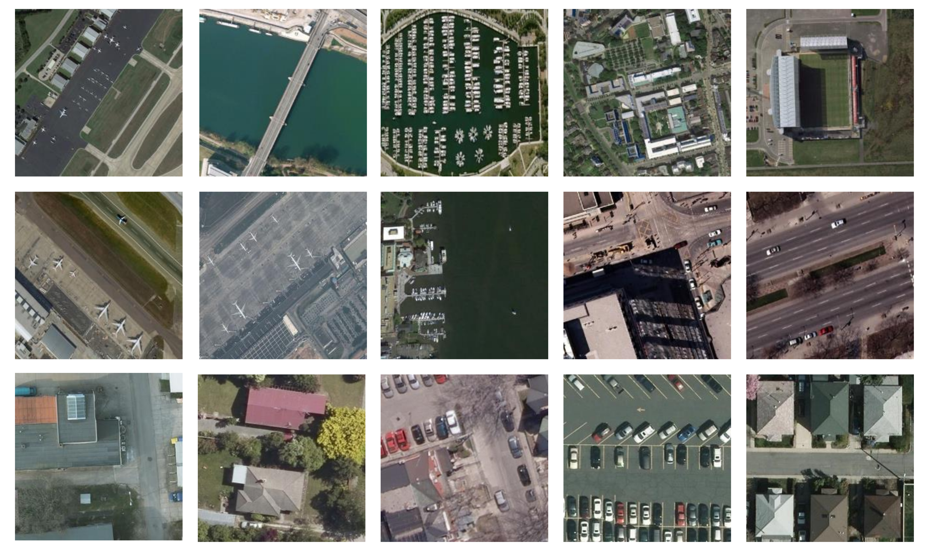
4.1.1. Dataset Settings
4.1.2. Evaluation Metrics
4.1.3. Implementation Details
4.2. Results and Analysis
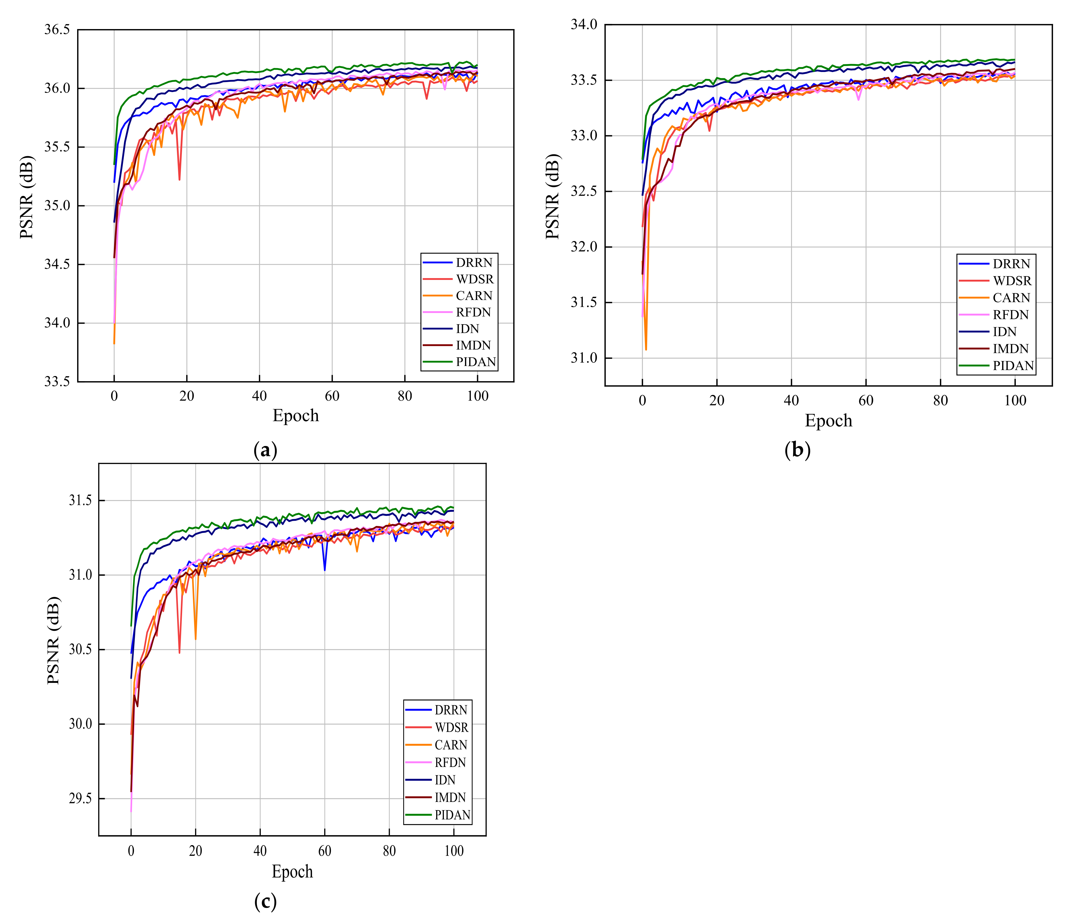
4.2.1. Comparison with Other Approaches
4.2.2. Model Size Analyses
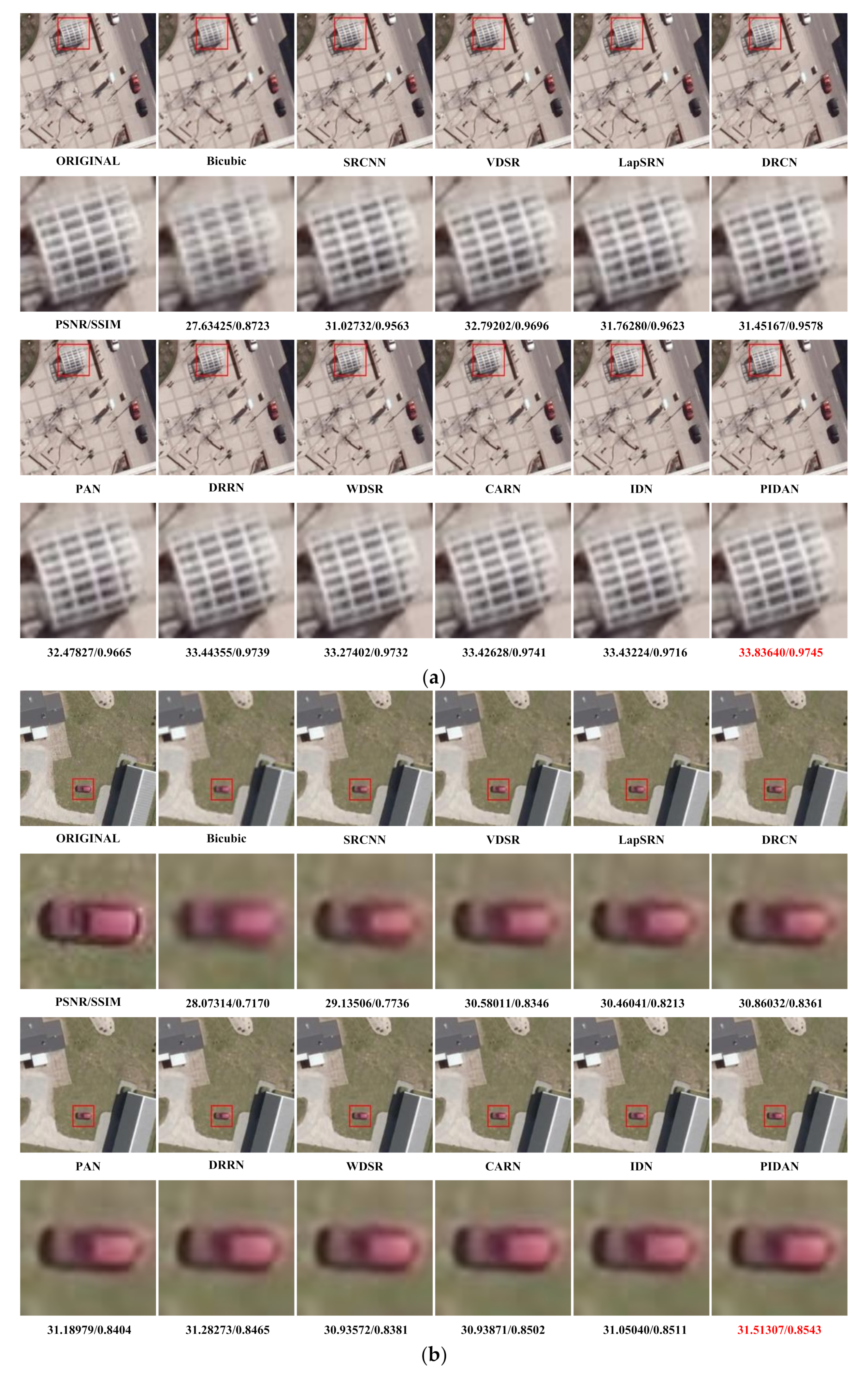
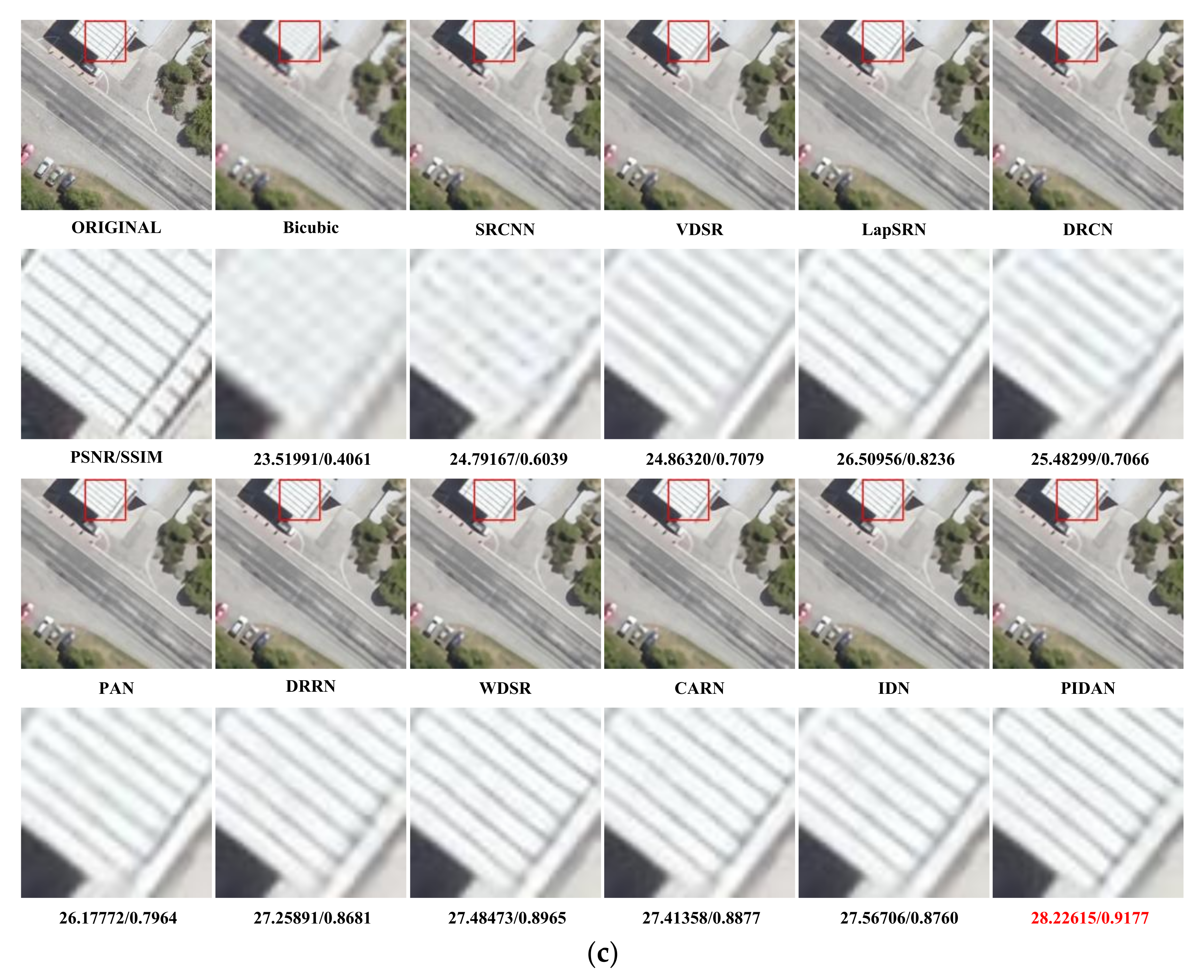
4.2.3. Visual Effect Comparison
4.2.4. Analysis of PIDAB
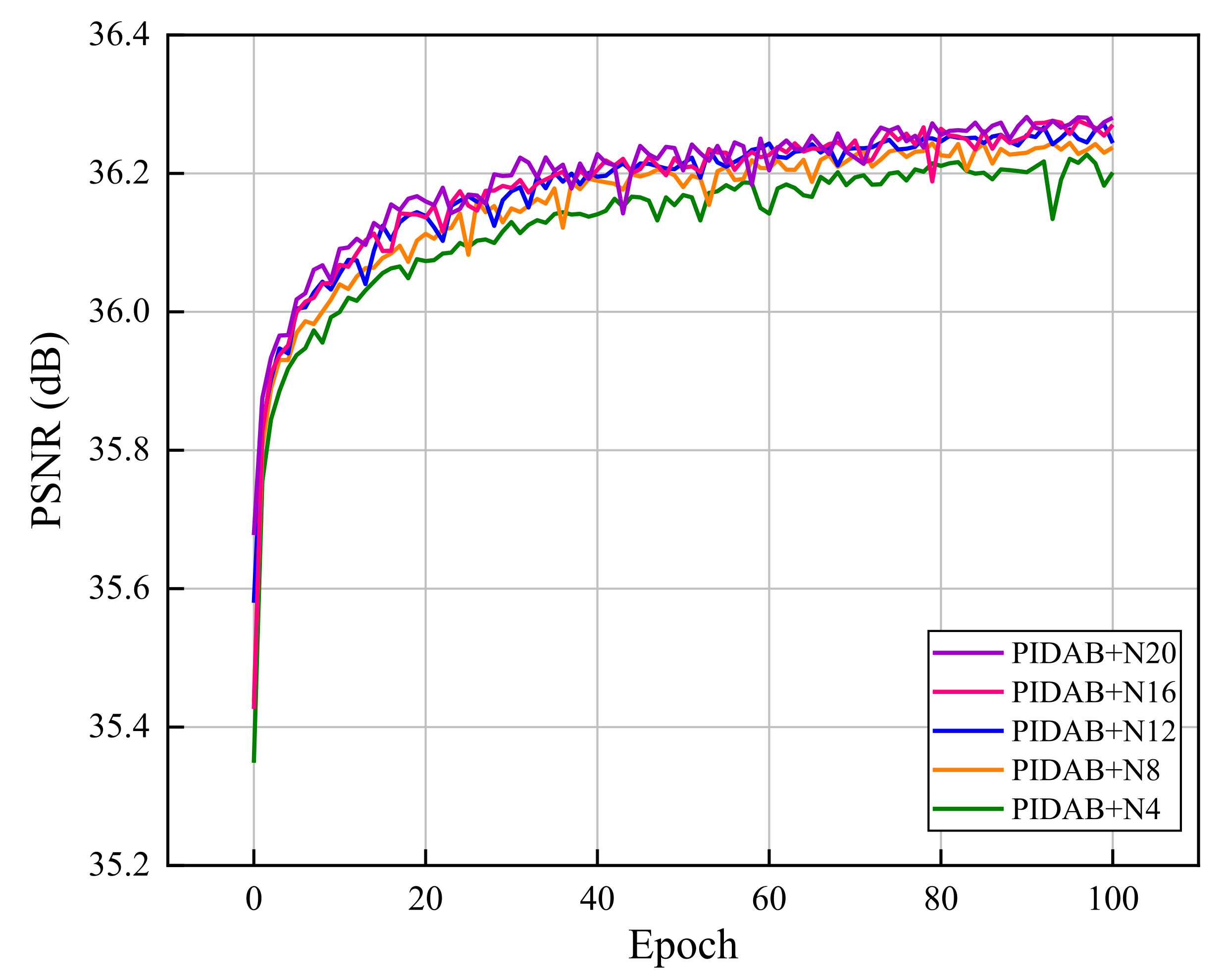
4.2.5. Effect of Number of PIDABs
5. Conclusions
Author Contributions
Funding
Institutional Review Board Statement
Informed Consent Statement
Data Availability Statement
Acknowledgments
Conflicts of Interest
References
- Som-ard, J.; Atzberger, C.; Izquierdo-Verdiguier, E.; Vuolo, F.; Immitzer, M. Remote sensing applications in sugarcane cultivation: A review. Remote Sens. 2021, 13, 4040. [Google Scholar] [CrossRef]
- Glasner, D.; Bagon, S.; Irani, M. Super-resolution from a single image. In Proceedings of the 2009 IEEE 12th International Conference on Computer Vision, Kyoto, Japan, 29 September–2 October 2009; pp. 349–356. [Google Scholar]
- Chang, H.; Yeung, D.; Xiong, Y. Super-resolution through neighbor embedding. In Proceedings of the 2004 IEEE Computer Society Conference on Computer Vision and Pattern Recognition, Washington, DC, USA, 27 June–2 July 2004; pp. 275–282. [Google Scholar]
- Zhang, L.; Wu, X. An edge-guided image interpolation algorithm via directional filtering and data fusion. IEEE Trans. Image Process. 2006, 15, 2226–2238. [Google Scholar] [CrossRef] [PubMed] [Green Version]
- Zhang, K.; Gao, X.; Tao, D.; Li, X. Single image super-resolution with non-local means and steering kernel regression. IEEE Trans. Image Process. 2012, 21, 4544–4556. [Google Scholar] [CrossRef] [PubMed]
- Protter, M.; Elad, M.; Takeda, H.; Milanfar, P. Generalizing the nonlocal-means to super-resolution reconstruction. IEEE Trans. Image Process. 2009, 18, 36–51. [Google Scholar] [CrossRef] [PubMed] [Green Version]
- Freeman, W.; Jones, T.; Pasztor, E. Example-based super-resolution. IEEE Comput. Graph. Appl. 2002, 22, 56–65. [Google Scholar] [CrossRef] [Green Version]
- Mu, G.; Gao, X.; Zhang, K.; Li, X.; Tao, D. Single image super resolution with high resolution dictionary. In Proceedings of the 2011 18th IEEE Conference on Image Processing, Brussels, Belgium, 11–14 September 2011; pp. 1141–1144. [Google Scholar]
- Dong, C.; Loy, C.; He, K.; Tang, X. Image super-resolution using deep convolutional networks. IEEE Trans. Pattern Anal. Mach. Intell. 2015, 38, 295–307. [Google Scholar] [CrossRef] [PubMed] [Green Version]
- Kim, J.; Lee, J.; Lee, K. Accurate image super-resolution using very deep convolutional networks. In Proceedings of the Conference on Computer Vision and Pattern Recognition, Las Vegas, NY, USA, 27–30 June 2016; pp. 1646–1654. [Google Scholar]
- Lim, B.; Son, S.; Kim, H.; Nah, S.; Lee, K.M. Enhanced deep residual networks for single image super-resolution. In Proceedings of the IEEE Conference on Computer Vision and Pattern Recognition Workshops, Honolulu, HI, USA, 21–26 July 2017; pp. 1132–1140. [Google Scholar]
- Zhang, Y.; Li, K.; Li, K.; Wang, L.; Zhong, B.; Fu, Y. Image super-resolution using very deep residual channel attention networks. In Proceedings of the European Conference on Computer Vision, Munich, Germany, 8–14 September 2018; pp. 286–301. [Google Scholar]
- Ledig, C.; Theis, L.; Huszár, F.; Caballero, J.; Cunningham, A.; Acosta, A.; Aitken, A.; Tejani, A.; Totz, J.; Wang, Z.; et al. Photorealistic single image super-resolution using a generative adversarial network. In Proceedings of the Conference on Computer Vision and Pattern Recognition, Honolulu, HI, USA, 21–26 July 2017; pp. 4681–4690. [Google Scholar]
- Zeng, K.; Yu, J.; Wang, R.; Li, C.; Tao, D. Coupled deep autoencoder for single image super-resolution. IEEE Trans. Cybern. 2017, 47, 27–37. [Google Scholar] [CrossRef] [PubMed]
- Hu, J.; Shen, L.; Sun, G. Squeeze-and-excitation networks. In Proceedings of the IEEE Conference on Computer Vision and Pattern Recognition, Salt Lake City, UT, USA, 18–22 June 2018; pp. 7132–7141. [Google Scholar]
- Zhang, D.; Shao, J.; Li, X.; Shen, H.T. Remote sensing image super-resolution via mixed high-order attention network. IEEE Trans. Geosci. Remote Sens. 2021, 59, 5183–5196. [Google Scholar] [CrossRef]
- Szegedy, C.; Liu, W.; Jia, Y.; Sermanet, P.; Reed, S.; Anguelov, D.; Erhan, D.; Vanhoucke, V.; Rabinovich, A. Going deeper with convolutions. In Proceedings of the IEEE Conference on Computer Vision and Pattern Recognition, Boston, MA, USA, 7–12 June 2015; pp. 1–9. [Google Scholar]
- Hui, Z.; Wang, X.; Gao, X. Fast and accurate single image super-resolution via information distillation network. In Proceedings of the IEEE Conference on Computer Vision and Pattern Recognition, Salt Lake City, UT, USA, 18–22 June 2018; pp. 723–731. [Google Scholar]
- Dun, Y.; Da, Z.; Yang, S.; Qian, X. Image super-resolution based on residually dense distilled attention network. Neurocomputing 2021, 443, 47–57. [Google Scholar] [CrossRef]
- Woo, S.; Park, J.; Lee, J.Y. CBAM: Convolutional Block Attention Module; Springer: Cham, Switzerland, 2018; p. 112211. [Google Scholar]
- Dong, C.; Loy, C.; Tang, X. Accelerating the super-resolution convolutional neural network. In Proceedings of the European Conference on Computer Vision, Amsterdam, The Netherlands, 8–16 October 2016; pp. 391–407. [Google Scholar]
- Shi, W.; Caballero, J.; Huszar, F.; Totz, J.; Aitken, A.; Bishop, R.; Rueckert, D.; Wang, Z. Real-time single image and video super-resolution using an efficient sub-pixel convolutional neural network. In Proceedings of the IEEE Conference on Computer Vision and Pattern Recognition, Las Vegas, NV, USA, 27–30 June 2016; pp. 1874–1883. [Google Scholar]
- He, K.M.; Zhang, X.Y.; Ren, S.Q.; Sun, J. Deep residual learning for image recognition. In Proceedings of the IEEE Conference on Computer Vision and Pattern Recognition, Las Vegas, NV, USA, 27–30 June 2016; pp. 770–778. [Google Scholar]
- Kim, J.; Lee, J.; Lee, K. Deeply-recursive convolutional network for image super-resolution. In Proceedings of the Conference on Computer Vision and Pattern Recognition, Las Vegas, NV, USA, 26 June–1 July 2016; pp. 1637–1645. [Google Scholar]
- Tai, Y.; Yang, J.; Liu, X. Image super-resolution via deep recursive residual network. In Proceedings of the IEEE Conference on Computer Vision and Pattern Recognition, Honolulu, HI, USA, 21–26 July 2017; pp. 3147–3155. [Google Scholar]
- Lai, W.; Huang, J.; Ahuja, J.; Yang, M. Deep Laplacian pyramid networks for fast and accurate super-resolution. In Proceedings of the Conference on Computer Vision and Pattern Recognition, Honolulu, HI, USA, 21–26 July 2017; pp. 624–632. [Google Scholar]
- Tong, T.; Li, G.; Liu, X.; Gao, Q. Image super-resolution using dense skip connections. In Proceedings of the IEEE International Conference on Computer Vision, Venice, Italy, 22–29 October 2017; pp. 4809–4817. [Google Scholar]
- Zhang, Y.; Tian, Y.; Kong, Y.; Zhong, B.; Fu, Y. Residual dense network for image super-resolution. In Proceedings of the IEEE Conference on Computer Vision and Pattern Recognition, Salt Lake City, UT, USA, 18–23 June 2018; pp. 2472–2481. [Google Scholar]
- Yu, J.; Fan, Y.; Yang, J.; Xu, N.; Wang, Z.; Wang, X.; Huang, T. Wide activation for efficient and accurate image super-resolution. arXiv 2018, arXiv:1808.08718. [Google Scholar]
- Ahn, N.; Kang, B.; Sohn, K.A. Fast, accurate, and lightweight super-resolution with cascading residual network. In Proceedings of the European Conference on Computer Vision, Munich, Germany, 8–14 September 2018; pp. 252–268. [Google Scholar]
- Buades, A.; Coll, B.; Morel, J. A non-local algorithm for image denoising. In Proceedings of the IEEE Computer Society Conference on Computer Vision and Pattern Recognition, San Diego, CA, USA, 20–25 June 2005; pp. 60–65. [Google Scholar]
- Wang, X.; Girshick, R.; Gupta, A.; He, K. Non-local neural networks. In Proceedings of the IEEE/CVF Conference on Computer Vision and Pattern Recognition, Salt Lake City, UT, USA, 18–23 June 2018; pp. 7794–7803. [Google Scholar]
- Cao, Y.; Xu, J.; Lin, S.; Wei, F.; Hu, H. GCNet: Non-local networks meet squeeze-excitation networks and beyond. In Proceedings of the IEEE/CVF International Conference on Computer Vision Workshop, Seoul, Korea, 27–28 October 2019; pp. 1971–1980. [Google Scholar]
- Zhang, Y.; Li, K.; Li, K.; Zhong, B.; Fu, Y. Residual non-local attention networks for image restoration. arXiv 2019, arXiv:1903.10082. [Google Scholar]
- Anwar, S.; Barnes, N. Densely residual Laplacian super-resolution. arXiv 2019, arXiv:1906.12021. [Google Scholar] [CrossRef] [PubMed]
- Guo, J.; Ma, S.; Guo, S. MAANet: Multi-view aware attention networks for image super-resolution. arXiv 2019, arXiv:1904.06252. [Google Scholar]
- Dai, T.; Cai, J.; Zhang, Y.; Xia, S.-T.; Zhang, L. Second-order attention network for single image super-resolution. In Proceedings of the IEEE Conference on Computer Vision and Pattern Recognition, Long Beach, CA, USA, 16–20 June 2019; pp. 11065–11074. [Google Scholar]
- Hui, Z.; Gao, X.; Yang, Y.; Wang, X. Lightweight image super-resolution with information multi-distillation network. In Proceedings of the 27th ACM International Conference on Multimedia, Nice, France, 21–25 October 2019; Volume 10, pp. 2024–2032. [Google Scholar]
- Zhao, H.; Kong, X.; He, J.; Qiao, Y.; Dong, C. Efficient image super-resolution using pixel attention. arXiv 2020, arXiv:2010.01073. [Google Scholar]
- Wang, H.; Wu, C.; Chi, J.; Yu, X.; Hu, Q.; Wu, H. Image super-resolution using multi-granularity perception and pyramid attention networks. Neurocomputing 2021, 443, 247–261. [Google Scholar] [CrossRef]
- Huang, B.; He, B.; Wu, L.; Guo, Z. Deep residual dual-attention network for super-resolution reconstruction of remote sensing images. Remote Sens. 2021, 13, 2784. [Google Scholar] [CrossRef]
- Xia, G.-S.; Hu, J.; Hu, F.; Shi, B.; Bai, X.; Zhong, Y.; Zhang, L. AID: A benchmark data det for performance evaluation of aerial scene classification. IEEE Trans. Geosci. Remote Sens. 2017, 55, 3965–3981. [Google Scholar] [CrossRef] [Green Version]
- Cheng, G.; Zhou, P.; Han, J. Learning rotation-invariant convolutional neural networks for object detection in VHR optical remote sensing images. IEEE Trans. Geosci. Remote Sens. 2016, 54, 7405–7415. [Google Scholar] [CrossRef]
- Mundhenk, T.N.; Konjevod, G.; Sakla, W.A.; Boakye, K. A large contextual dataset for classification, detection and counting of cars with deep learning. In European Conference on Computer Vision; Springer: Cham, Switzerland, 2016; pp. 785–800. [Google Scholar]
- Horé, A.; Ziou, D. Image quality metrics: PSNR vs. SSIM. In Proceedings of the International Conference on Computer Vision, Istanbul, Turkey, 23–26 August 2010; pp. 2366–2369. [Google Scholar]
- Wang, Z.; Bovik, A.C.; Sheikh, H.R.; Simoncelli, E.P. Image quality assessment: From error visibility to structural similarity. IEEE Trans. Image Process. 2004, 13, 600–612. [Google Scholar] [CrossRef] [PubMed] [Green Version]
- Kingma, D.P.; Ba, J.L. Adam: A method for stochastic optimization. In Proceedings of the 3rd International Conference on Learning Representations, San Diego, CA, USA, 7–9 May 2015. [Google Scholar]
- Liu, J.; Tang, J.; Wu, G. Residual feature distillation network for lightweight image super-resolution. arXiv 2020, arXiv:2009.11551. [Google Scholar]

| Structure Component | Layer | Input | Output |
|---|---|---|---|
| M1 | Conv3 × 3 | H × W × 64 | H × W × 48 |
| M2 | Conv3 × 3 | H × W × 48 | H × W × 32 |
| M3 | Conv3 × 3 | H × W × 32 | H × W × 64 |
| PCCS | Conv3 × 3 | H × W × 64 | H × W × 64 |
| Split | H × W × 64 | H × W × 48, H × W × 16 | |
| Conv5 × 5 | H × W × 64 | H × W × 64 | |
| Split | H × W × 64 | H × W × 48, H × W × 16 | |
| Conv7 × 7 | H × W × 64 | H × W × 64 | |
| Split | H × W × 64 | H × W × 48, H × W × 16 | |
| Sum | H × W × 48, H × W × 48, H × W × 48 | H × W × 48 | |
| Sum | H × W × 16, H × W × 16, H × W × 16 | H × W × 16 | |
| Concat | H × W × 64, H × W × 16 | H × W × 80 | |
| HAM | GAP | H × W × 80 | 1 × 1 × 80 |
| Conv1 × 1 | 1 × 1 × 80 | 1 × 1 × 5 | |
| Conv1 × 1 | 1 × 1 × 5 | 1 × 1 × 80 | |
| Multiple | H × W × 80, 1 × 1 × 80 | H × W × 80 | |
| AvgPool | H × W × 80 | H × W × 1 | |
| MaxPool | H × W × 80 | H × W × 1 | |
| Concat | H × W × 1, H × W × 1 | H × W × 2 | |
| Conv7 × 7 | H × W × 2 | H × W × 1 | |
| Multiple | H × W × 80, H × W × 1 | H × W × 80 | |
| Sum | H × W × 80, H × W × 80, H × W × 80 | H × W × 80 | |
| M4 | Conv3 × 3 | H × W × 48 | H × W × 64 |
| M5 | Conv3 × 3 | H × W × 64 | H × W × 48 |
| M6 | Conv3 × 3 | H × W × 48 | H × W × 80 |
| Sum | H × W × 80, H × W × 80 | H × W × 80 | |
| CC unit | Conv1 × 1 | H × W × 80 | H × W × 64 |
| NWPU VHR-10 | COWC | |||||
|---|---|---|---|---|---|---|
| Method | PSNR/SSIM | PSNR/SSIM | ||||
| ×2 | ×3 | ×4 | ×2 | ×3 | ×4 | |
| Bicubic | 32.76031/0.8991 | 29.90444/0.8167 | 28.28280/0.7524 | 32.87844/0.9180 | 29.53540/0.8384 | 27.72172/0.7725 |
| SRCNN | 34.03260/0.9136 | 30.97869/0.8400 | 29.20195/0.7793 | 35.05635/0.9341 | 31.14172/0.8661 | 28.99814/0.8058 |
| VDSR | 34.46067/0.9196 | 31.46934/0.8517 | 29.62497/0.7931 | 35.81885/0.9401 | 31.89712/0.8788 | 29.62051/0.8220 |
| LapSRN | 34.24569/0.9169 | 31.26756/0.8468 | 29.67748/0.7942 | 35.48608/0.9375 | 31.62203/0.8741 | 29.70046/0.8236 |
| DRCN | 34.36621/0.9181 | 31.31746/0.8476 | 29.51012/0.7887 | 35.65558/0.9387 | 31.67424/0.8751 | 29.46399/0.8180 |
| PAN | 34.48577/0.9199 | 31.53275/0.8529 | 29.75737/0.7967 | 35.86121/0.9403 | 31.98120/0.8800 | 29.80853/0.8262 |
| DRRN | 34.57956/0.9213 | 31.59945/0.8548 | 29.85024/0.8002 | 36.01337/0.9417 | 32.08846/0.8820 | 29.85881/0.8272 |
| WDSR | 34.56984/0.9210 | 31.65636/0.8558 | 29.87613/0.8003 | 36.01360/0.9416 | 32.17758/0.8832 | 30.00641/0.8305 |
| CARN | 34.54988/0.9208 | 31.59971/0.8545 | 29.83102/0.7990 | 35.97727/0.9413 | 32.07578/0.8817 | 29.93067/0.8289 |
| RFDN | 34.55302/0.9207 | 31.61688/0.8548 | 29.81638/0.7984 | 35.99849/0.9413 | 32.14530/0.8826 | 29.91353/0.8285 |
| IDN | 34.56317/0.9210 | 31.61978/0.8550 | 29.83245/0.7989 | 35.99732/0.9415 | 32.12127/0.8823 | 29.92513/0.8286 |
| IMDN | 34.55570/0.9207 | 31.62651/0.8549 | 29.81952/0.7984 | 36.02204/0.9415 | 32.17454/0.8829 | 29.95087/0.8291 |
| PIDAN | 34.59635/0.9215 | 31.66433/0.8559 | 29.87914/0.8005 | 36.09257/0.9423 | 32.23239/0.8840 | 30.00399/0.8303 |
| Scale | PCCS | HAM | NWPU VHR-10 | COWC |
|---|---|---|---|---|
| PSNR/SSIM | PSNR/SSIM | |||
| ×2 | ⨉ | ⨉ | 34.55616/0.9209 | 35.99601/0.9415 |
| ✓ | ⨉ | 34.58637/0.9214 | 36.03984/0.9419 | |
| ⨉ | ✓ | 34.57436/0.9211 | 36.03683/0.9417 | |
| ✓ | ✓ | 34.59635/0.9215 | 36.09257/0.9422 |
| Scale | Kernel Size | NWPU VHR-10 | COWC | ||
|---|---|---|---|---|---|
| 3 | 5 | 7 | PSNR/SSIM | PSNR/SSIM | |
| ×2 | ⨉ | ⨉ | ⨉ | 34.55616/0.9209 | 35.99601/0.9415 |
| ✓ | ⨉ | ⨉ | 34.57641/0.9212 | 36.02632/0.9418 | |
| ⨉ | ✓ | ⨉ | 34.57483/0.9212 | 36.01945/0.9418 | |
| ⨉ | ⨉ | ✓ | 34.57012/0.9212 | 36.02009/0.9418 | |
| ✓ | ✓ | ⨉ | 34.57821/0.9212 | 36.02750/0.9418 | |
| ✓ | ⨉ | ✓ | 34.58540/0.9213 | 36.03357/0.9419 | |
| ⨉ | ✓ | ✓ | 34.58416/0.9214 | 36.02602/0.9419 | |
| ✓ | ✓ | ✓ | 34.58637/0.9214 | 36.03984/0.9419 | |
| Scale | Approach | NWPU VHR-10 | COWC |
|---|---|---|---|
| PSNR/SSIM | PSNR/SSIM | ||
| ×2 | / | 34.55616/0.9209 | 35.99601/0.9415 |
| SE block | 34.56088/0.9209 | 36.02749/0.9416 | |
| CBAM | 34.56436/0.9211 | 36.03021/0.9416 | |
| HAM | 34.57436/0.9211 | 36.03683/0.9417 |
Publisher’s Note: MDPI stays neutral with regard to jurisdictional claims in published maps and institutional affiliations. |
© 2021 by the authors. Licensee MDPI, Basel, Switzerland. This article is an open access article distributed under the terms and conditions of the Creative Commons Attribution (CC BY) license (https://creativecommons.org/licenses/by/4.0/).
Share and Cite
Huang, B.; Guo, Z.; Wu, L.; He, B.; Li, X.; Lin, Y. Pyramid Information Distillation Attention Network for Super-Resolution Reconstruction of Remote Sensing Images. Remote Sens. 2021, 13, 5143. https://doi.org/10.3390/rs13245143
Huang B, Guo Z, Wu L, He B, Li X, Lin Y. Pyramid Information Distillation Attention Network for Super-Resolution Reconstruction of Remote Sensing Images. Remote Sensing. 2021; 13(24):5143. https://doi.org/10.3390/rs13245143
Chicago/Turabian StyleHuang, Bo, Zhiming Guo, Liaoni Wu, Boyong He, Xianjiang Li, and Yuxing Lin. 2021. "Pyramid Information Distillation Attention Network for Super-Resolution Reconstruction of Remote Sensing Images" Remote Sensing 13, no. 24: 5143. https://doi.org/10.3390/rs13245143
APA StyleHuang, B., Guo, Z., Wu, L., He, B., Li, X., & Lin, Y. (2021). Pyramid Information Distillation Attention Network for Super-Resolution Reconstruction of Remote Sensing Images. Remote Sensing, 13(24), 5143. https://doi.org/10.3390/rs13245143