Abstract
Deep learning has recently attracted extensive attention and developed significantly in remote sensing image super-resolution. Although remote sensing images are composed of various scenes, most existing methods consider each part equally. These methods ignore the salient objects (e.g., buildings, airplanes, and vehicles) that have more complex structures and require more attention in recovery processing. This paper proposes a saliency-guided remote sensing image super-resolution (SG-GAN) method to alleviate the above issue while maintaining the merits of GAN-based methods for the generation of perceptual-pleasant details. More specifically, we exploit the salient maps of images to guide the recovery in two aspects: On the one hand, the saliency detection network in SG-GAN learns more high-resolution saliency maps to provide additional structure priors. On the other hand, the well-designed saliency loss imposes a second-order restriction on the super-resolution process, which helps SG-GAN concentrate more on the salient objects of remote sensing images. Experimental results show that SG-GAN achieves competitive PSNR and SSIM compared with the advanced super-resolution methods. Visual results demonstrate our superiority in restoring structures while generating remote sensing super-resolution images.
1. Introduction
High spatial quality (HQ) optical remote sensing images have a high spatial resolution and low noise characteristics, which can be widely used in agricultural and forestry monitoring, urban planning, military surveillance, and other fields. However, the time and cost of development and the vulnerability of the image to the changes in atmosphere and light are the reasons for the acquisition of a large number of low spatial quality (LQ) remote sensing images. Recently, more researchers have poured attention into recovering HQ remote sensing images from LQ using image processing technology. Low spatial resolution is a crucial factor for the low quality of remote sensing images [1]. Therefore, enhancing spatial resolution became the most common approach to acquiring high-quality images.
Remote sensing image super-resolution (SR) aims to recover the high-resolution (HR) remote sensing image from the corresponding low-resolution (LR) remote sensing image. Currently, remote sensing image SR has become an intensely active research topic in remote sensing image analysis [2]. However, it is an ill-posed problem as each LR input may have multiple HR solutions. In traditional approaches, HR images are obtained by filling LR adopted interpolation methods, typically including the nearest neighbor and bicubic interpolation [3]. These methods only considered the surrounding pixels so that only a little valuable new information is added to the image. Then, the methods in [4,5] became competitive methods, which explore the neighbors of a patch in feature space to help reconstruct the high-resolution image. Due to the above approaches heavily relying on hand-crafted features, optimizing them is difficult and time-consuming. Afterward, the method in [6,7], based on dictionary learning, has also been well applied in image super-resolution tasks. Most of them are optimized by the mean squared error (MSE), which measures the pixel-wise distances between SR images and the HR ones. However, such optimizing objective impels models to produce a statistical average of possible HR solutions, the one-to-many problem. As a result, such methods usually generate blurry results with a low peak signal-to-noise ratio (PSNR).
With the development of deep learning, convolutional neural networks (CNNs) have shown great success in most computer vision areas [8]. In typical CNN-based SR methods, distortion-oriented loss functions are considered, attempting to achieve a higher PSNR and lower distortion in terms of MSE. There have been lots of distortion-oriented CNNs developed for SR [8,9,10], and the performance of SR is ever-improving as many researchers are still creating innovative architectures and as the possible depth and connections of the network are growing. However, they yield blurry results and do not recover the fine details even with intense and complex networks. The results of distortion-oriented models are the average of possible HR images.
To resolve the above-mentioned issues, perception-oriented models and generative adversarial network (GAN) [11] have been proposed for obtaining the HR images with better perceptual quality. For example, the perceptual loss was introduced in [12], which is defined as the distance in the feature domain. More recently, SRGAN [13] and EnhanceNet [14] have been proposed to improve perceptual quality. The SRGAN employed generative models and adopted the perceptual loss. The EnhancedNet added an additional texture loss [15] for better texture reconstruction. In [16], the authors proposed RRDGAN to acquire better-quality images by incorporating denoising and SR into a unified framework. The authors of [17] combined a cyclic generative network with residual feature aggregation to improve image super-resolution performance. Furthermore, the notion of GANs has been draw on a variety of fields, such as style-transfer [18,19,20], image dehazing [21], image completion [22], music generation [23], image segmentation [24], image classification [25], and image change detection [26].
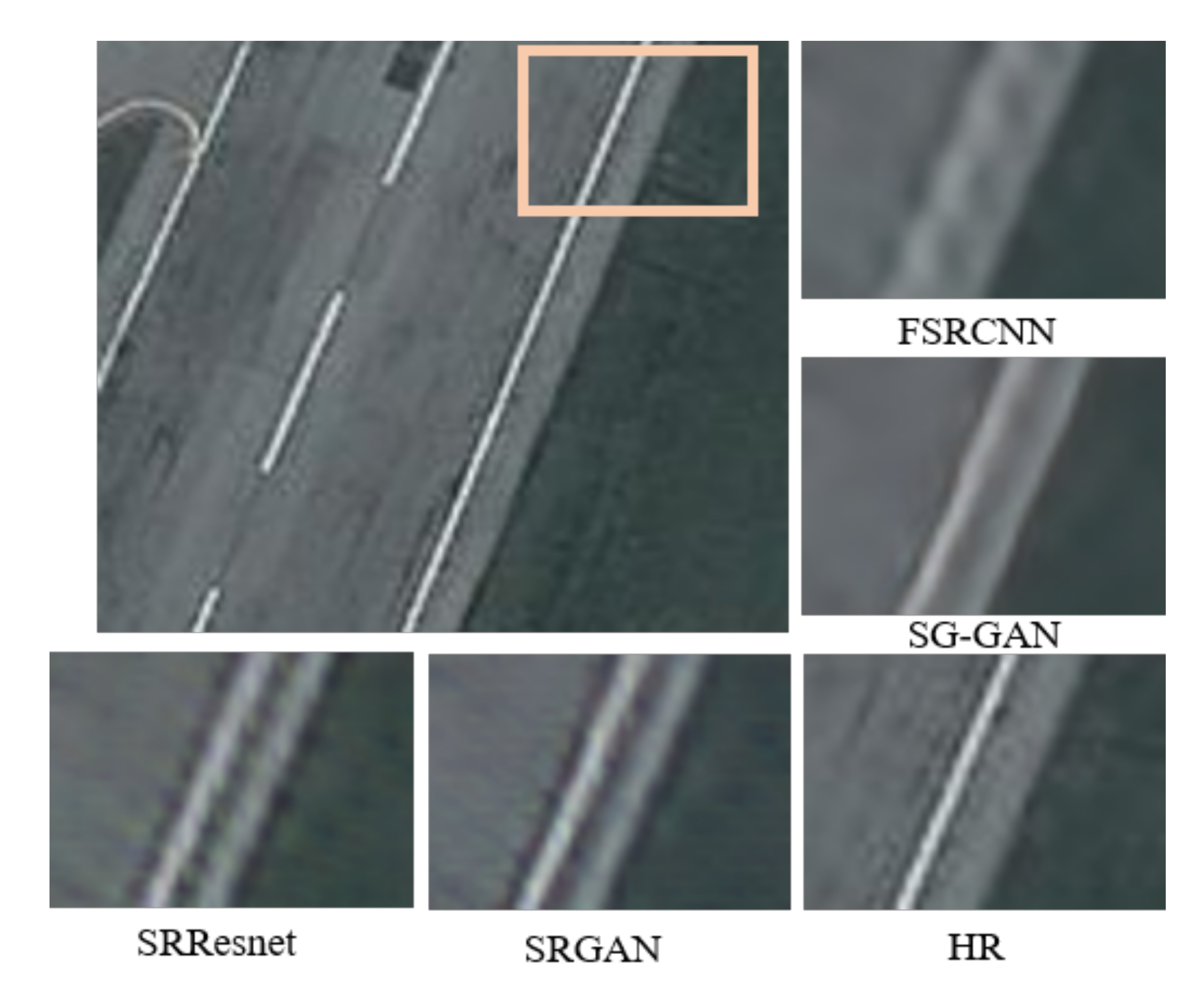
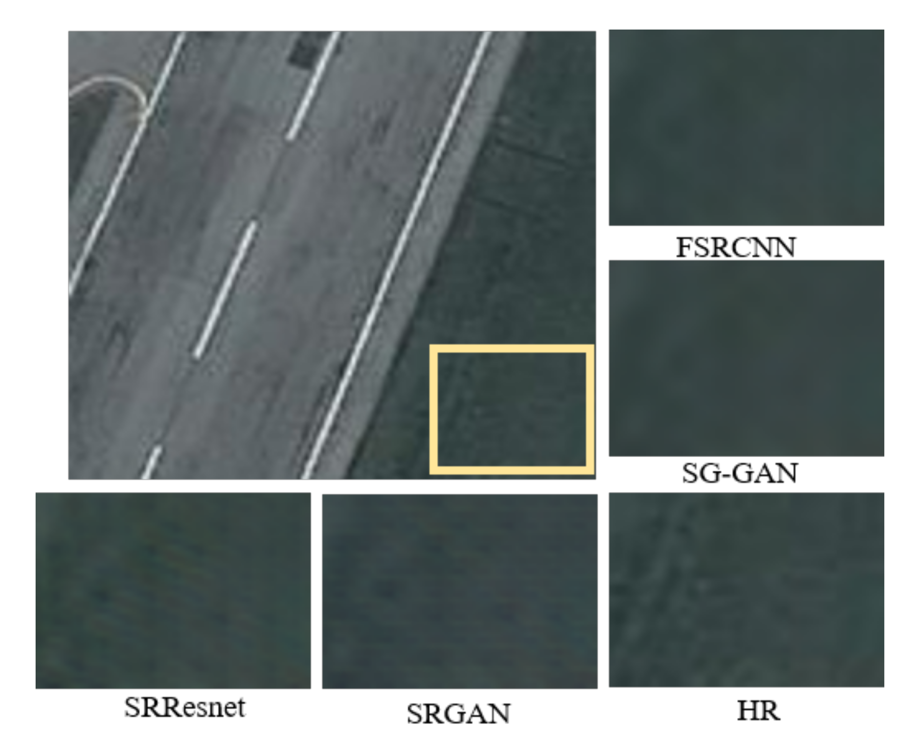
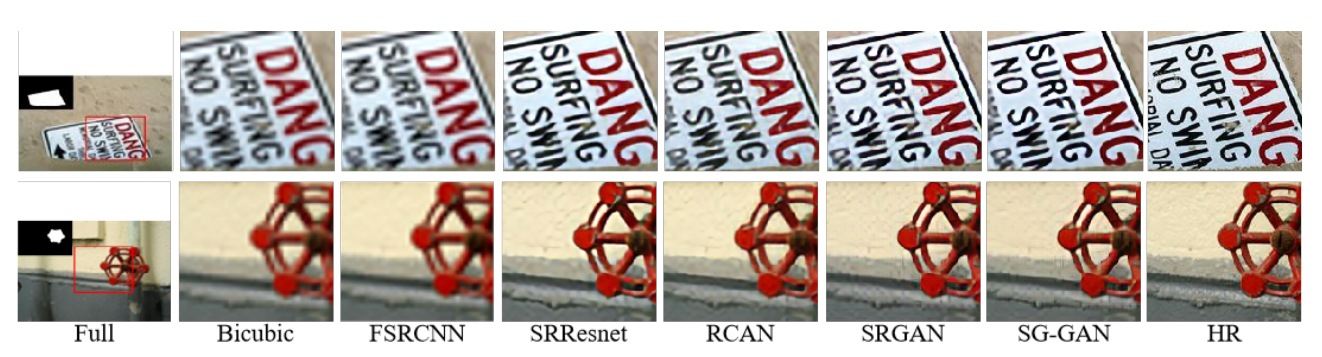
However, most remote sensing image SR methods regard each region equally, disregarding the difference between the contents of image regions, which could easily lead to suboptimal solutions. The background areas of some remote sensing images are known as non-saliency regions. In contrast, the region is expected to be “clear”, called a saliency region. More specifically, as shown in Figure 1, for the region of salient areas of the remote sensing image, different image SR methods will conduct considerably varies in the SR results. While no matter what method is adopted to recover the region within the box, the recovered result is not much different in Figure 2. Therefore, it is necessary to focus on recovering salient areas.
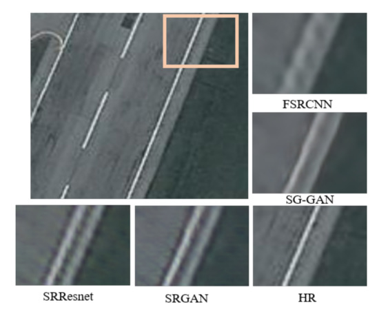
Figure 1.
Comparison of the results of different methods in the saliency region of remote sensing images.
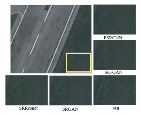
Figure 2.
Comparison of the results of different methods in the non-saliency region of remote sensing images.
Salient object detection (SOD) is a technique for extracting the regions with the most conspicuous and noticeable object [27], focusing on segmenting images to generate pixel-wise saliency maps [28]. Because of its low computational cost and impressive scalability, SOD has aroused interest in many fields, including image retrieval [29], object tracking [30], semantic segmentation [31], remote sensing segmentation [32], camouflage object detection [33], etc. In general, in the large-scale optical remote sensing images with cluttered and intricate noise, the SOD for remote sensing images aims to segment a few regions with noteworthy color, shape or texture. As a fundamental and preprocessing task, the SOD methods have been widely applied to various tasks of remote sensing images analysis, such as human-made object detection [34], change detection [35], and ROI extraction [36]. The traditional methods of detecting salient objects depend on handcrafted features, such as contrast [37] and boundary background [38]. With the rapid development of convolutional neural networks, an increasing number of researchers propose to estimate a saliency map from an image with end-to-end networks [39,40,41].
Based on the advantages of salient object detection, a proper saliency map helps boost super-resolution performance by allocating more resources to import regions accordingly. Therefore, this paper proposes a generative adversarial network with saliency-guided remote sensing image super-resolution (SG-GAN) to alleviate the above-mentioned issue. As the saliency map reveals the salient regions in an image, we apply this powerful tool to guide image recovery. This paper designs a saliency-guided network that aligns the saliency map estimated from the generated SR image with one of the HR images as an auxiliary SR problem. Then, the saliency map is integrated into the remote sensing SR network to guide the high-resolution image reconstruction. The main contributions of our paper can be summarized as follows.
- We propose a saliency-guided remote sensing image super-resolution network (SG-GAN) while maintaining the merits of GAN-based methods to generate perceptual-pleasant details. Additionally, the saliency object detection module with an encode–decoder structure in SG-GAN helps generative networks to focus training on the salient regions of the image.
- We provide the additional constraint to supervise the saliency map of the remote sensing images by designing a saliency loss. It imposed a second-order restriction in the SR process to retain the structural configuration and encourage the obtained SR images with higher perceptual quality and fewer geometric distortions.
- Compared with the existing methods, the SG-GAN model reconstructs high-quality details and edges in transformed images, both quantitatively and qualitatively.
In the rest of the paper, we briefly review related works in Section 2. In Section 3, the main idea of the proposed method, network structure, and loss functions are introduced in detail. Specific experimental design and comparison of experimental results are shown in Section 4. Section 5 conducts a particular analysis of the experimental results. At last, Section 6 makes a summary of the paper.
2. Related Works
This section mainly introduces related deep learning-based image super-resolution and salient object detection.
2.1. Deep Learning-Based Image Super-Resolution
The deep learning-based image super-resolution methods are usually divided into two frameworks: One is image super-resolution with convolutional neural networks, and the other is image super-resolution with generative adversarial networks.
2.1.1. Image Super-Resolution with Convolutional Neural Networks
The groundbreaking work of image super-resolution came from SRCNN [8] in 2014. SRCNN implemented an end-to-end mapping by using three convolutional layers. These three layers had completed the task of feature extraction and high-resolution image reconstruction. FSRCNN [42] was an improved version of SRCNN. Instead of inputting high-dimensional images, the FSRCNN directly extracted features from LR images and utilized deconvolution to upscale images. There are many models [43,44,45] that rely on residual connection methods and have achieved good results. RCAN [46] introduced the attention mechanism to image super-resolution to improve feature utilization. Chen et al. designed a self-supervised spectral-spatial residual network [47]. The authors of [48] proposed multi-scale dilation residual block to deal with the super-resolution problem of remote sensing images.
2.1.2. Image Super-Resolution with Generative Adversarial Networks
The generative adversarial network [11] was proposed by Goodfellow et al. in 2014, which has been widely applied in numerous visual tasks. In the field of image super-resolution, Ledig et al. proposed SRGAN [13], which adopted GAN to implement image super-resolution tasks. SRGAN exploited residual network [49] structure as the main structure for the generator. Skip connection operation to add low-resolution information directly to the learned high-dimension features. VGG [50] network was utilized in the main body of the discriminator, which guided the generator to pay plenty of attention to in-depth features. Under the GAN framework, the adversarial loss was also an effective loss to improve image resolution by minimizing the differences between generated images and target images. Ref. [51] proposed an Enlighten-GAN model, which utilized the Self-Supervised Hierarchical Perceptual Loss to optimize network results. Both the works in [52,53] have achieved outstanding results based on GAN. Although these existing perceptual-driven methods indeed improve the overall visual quality of super-resolved images, they equally consider whether saliency regions or non-saliency regions in remote sensing images.
2.2. Region-Aware Image Restoration
Gu et al. [54] suggest that the performance difference of various methods mainly lies in the areas with complex structure and rich texture. Recently, researchers have proposed various strategies for other regions of images to achieve better image processing results. RAISE [55] divides the low-resolution images into different image clusters and designs specific filters for each image cluster. SFTGAN [56] introduces a spatial feature transformation layer, combining the advanced semantic information with the image’s features. ClassSR [57] proposes a classification-based method to classify the image blocks according to the restoration difficulty and adopts different super-resolution networks to improve the super-resolution efficiency and super-resolution effect. The difference is that this paper proposes a super-resolution network based on the saliency guidance, which enhances the super-resolution effect by providing additional constraints to the saliency region of the image and assigning more weights.
2.3. Salient Object Detection
With the rapid development of convolutional neural networks, an increasing number of researchers classified images into the saliency area and non-saliency area by utilizing super-pixels or local patches. MACL [58] adopted two paths to extract local and global contexts from different windows of super-pixels and then built a united model in the same hybrid deep learning framework. The work in [59] combined abstraction, element distribution, and uniqueness to obtain a saliency map to construct a saliency loss to deal with retinal vasculature image super-resolution. Qin et al. proposed BASNet [60] to segment the salient object regions, which predicted the structures with clear boundaries. Saliency information may provide additional supervision for better image reconstruction for deep adversarial networks. In this work, we aim to leverage saliency-guided to further improve the GAN-based remote sensing SR methods.
3. Proposed Methods
In this section, we first present the proposed SG-GAN framework in detail. Then salient object detection model is demonstrated. Finally, the optimization function is introduced briefly.
Based on the above analysis, recovering the salient regions of an image play an essential role in improving the performance of remote sensing image super-resolution tasks. This paper focuses on detecting the salient regions and paying more attention to these regions. Figure 3 shows our main idea. We adopt the salient object detection network to detect the generated image’s saliency map and the target image’s saliency map to motivate SG-GAN to recover more structure details.
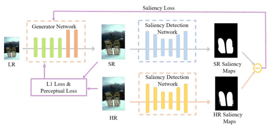
Figure 3.
The main idea of SG-GAN: the low-resolution images are input into the generator, then output into super-resolution images. The generated and authentic images are input into the salient object detection network separately. The discrepancy of the two saliency maps estimated from generated and HR images is encoded as saliency loss. The loss is fed back to the generator, making the saliency area of the generated image more realistic.
3.1. Structure of SG-GAN
SG-GAN consists of two parts: the generator and the discriminator. The generator can reconstruct the input low-resolution image into a super-resolution image. The discriminator acts as a leader, guiding the generator to generate a direction closer to the high-resolution image for training.
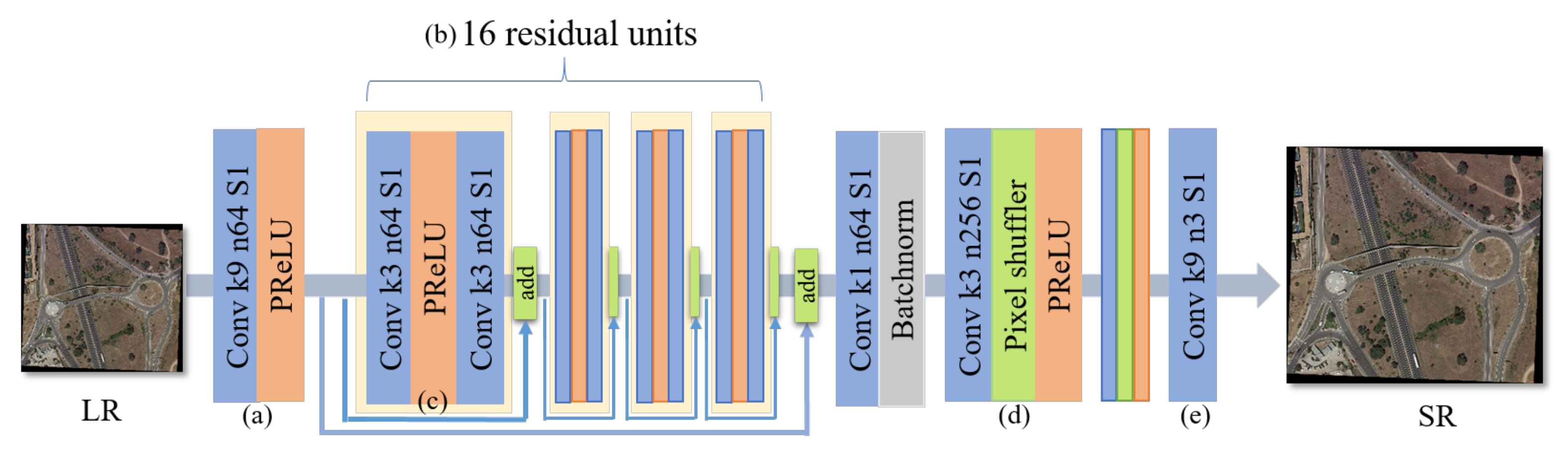
As shown in Figure 4, the generator mainly contains five parts: (a) shallow feature extraction unit, (b) deep feature extraction unit, (c) reducing parameters unit, (d) upscaling unit, and (e) image reconstruction unit. Precisely, for (a), the generator extracts the shallow feature by utilizing a convolution layer with the kernel size of 9 and a ParametricReLU layer [61] as the activate function, which converts the image of three channels into a feature map with 64 channels. (b) Then, through the 16 residual units for deep feature extraction, which have been proposed in [62], extracting the low, medium, and high-frequency features for more abundant information. (c) The residual blocks (RB) remove the batch normalization layer to save memory and reduce parameters. Moreover, the generator employs a short and long skip connection to transfer the shallow feature directly to in-depth features, thereby achieving the fusion of the low-level and high-level features. Then, all the extracted features are converted by a convolution layer with a kernel size. In order to prepare for the subsequent upsampling operation, the number of features is integrated and reduced. (d) Finally, two sub-pixel convolutions contain the convolution layer, Pixel shuffle, and PReLU, which can be regarded as the upscaling unit. (e) The final remote sensing super-resolution image is obtained through a convolution layer of kernel size.
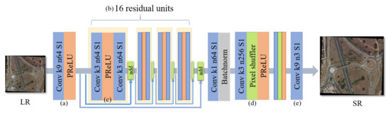
Figure 4.
SG-GAN generator structure diagram with corresponding kernel size, number of feature maps, and stride for each convolutional layer. It can be seen as five parts: (a) shallow feature extraction, (b) deep feature extraction, (c) reducing parameters, (d) upscaling unit, and (e) image reconstruction.
The discriminator network is trained to discriminate authentic HR images from generated SR samples. It adopts the exact structure of SRGAN in the discriminator module to pay more attention to the deep parts and to solve the maximization problem in Equation (1). The discriminator structure is shown in Figure 5. Specifically, the input image passes through 8 convolutional layers with an increasing number of filter kernels, increasing by a factor of 2 from 64 to 512 kernels in-depth feature information. The discriminator considers the authenticity of the deep feature information. At the end of the discriminator, a number between 0 and 1 is obtained through the Sigmoid function. Then, the size of the number judges the authentic degree of the input image. When the output number is between 0 and , the input image is fake; when the output number is between and 1, the input image is an actual image. As deep features help improve the sharpness of the image, the generator can generate a sharper image under the guidance of the discriminator.
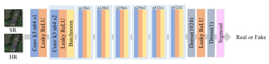
Figure 5.
SG-GAN discriminator structure diagram with corresponding kernel size, number of feature maps, and stride for each convolutional layer. The discriminator expresses the authenticity of the input image by outputting numbers.
3.2. Details of Salient Object Detection Network
As shown in Figure 3, the remote sensing SR network incorporates saliency regions representations from the salient object detection network. The motivation of this scheme is that the more accurate the grasp of saliency regions, the more helpful it is to reconstruct the resolution of complex areas. A well-designed saliency object detection branch can carry rich saliency information, which is pivotal to recovering remote sensing image SR.
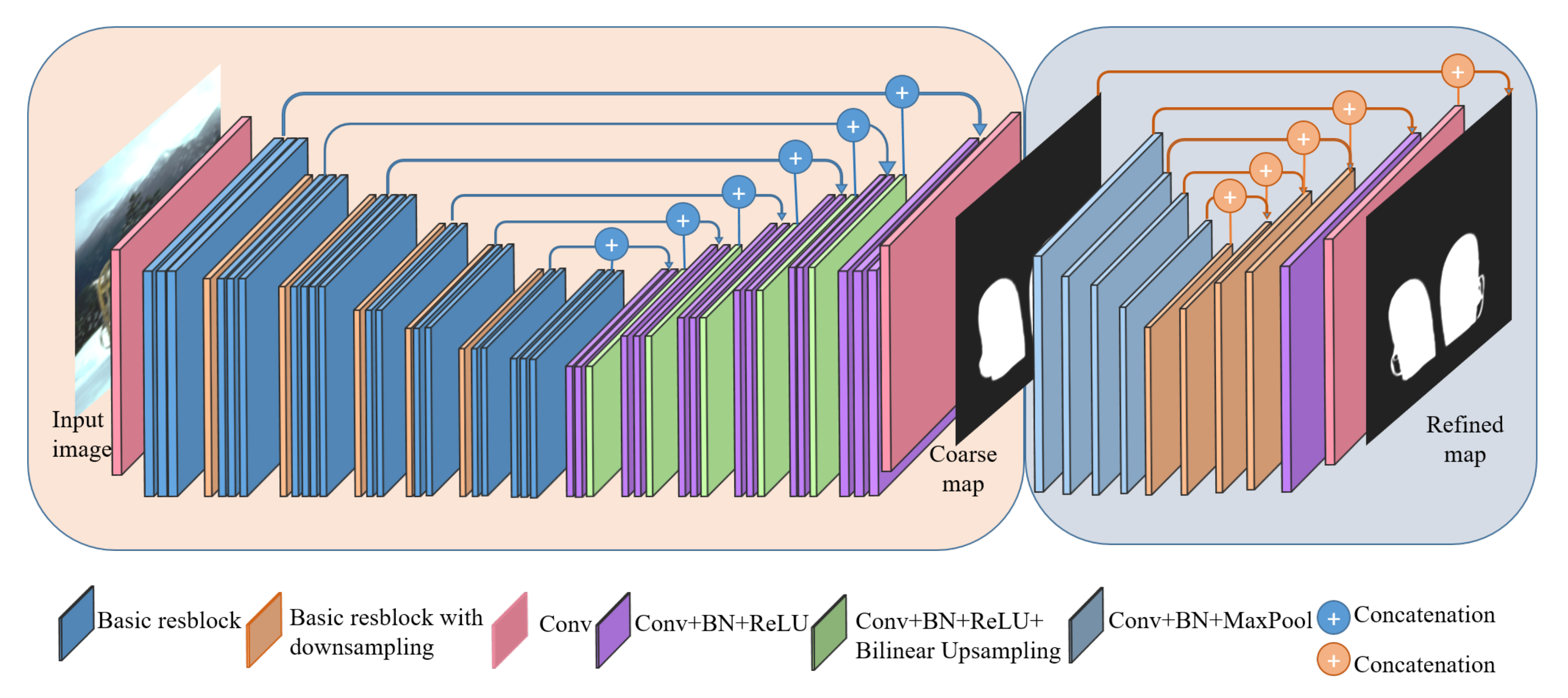
Salient object detection methods based on Fully Convolutional Neural Networks (FCN) are able to capture richer spatial and multiscale information to retain the location information and obtain structure features. In this paper, BASNet [60] is selected as the salient object detection network baseline. Inspired by U-Net, we design our salient object prediction module as an Encoder–Decoder network in Figure 6 because this kind of architecture is able to capture high-level global contexts and low-level details at the same time. Meanwhile, spatial location information is also captured. The existence of a bridge structure helps the whole network to capture the global feature. The output is a salient object with a distinct edge from the last layer of the network. Moreover, in order to accurately predict the saliency areas and their contours, the paper applies a hybrid loss ℓ in Equation (2) which contains Binary Cross-Entropy (BCE) in Equation (3), Structural Similarity (SSIM) in Equation (4) and Intersection-over-Union (IoU) loss in Equation (5) to achieved superior performance at pixel-level, patch-level, and map-level.
where , , and denote BCE loss [63], SSIM loss [64], and IoU loss [65], respectively.

Figure 6.
Diagram of salient object detection network structure.
BCE loss is the most widely used loss in binary classification and segmentation. It is defined as
where denotes the ground-truth label of pixel and denotes the predicted probability of being the salient object, measuring the pixel-wise level.
SSIM is originally proposed for image quality assessment, which captures the structural information in an image. Therefore, we integrated it into our saliency detection training loss to learn the structural information of the salient object ground truth. Suppose and be the pixel values of two corresponding patches, which size are cropped from the predicted probability map S and the binary ground truth mask G respectively, the SSIM of x and y is defined as
where , and , denote the mean and standard deviations of x and y, respectively, denotes the covariance of x and y, and are used to refrain from dividing by zero, measuring the patch-wise level.
IoU measures the similarity of two sets [66] and as a standard evaluation measure for object detection and segmentation. To ensure its differentiability, we adopt the IoU loss used in [64]:
where denotes the ground-truth label of the pixel and is the predicted probability of being the salient object, measuring the map-wise level.
Based on the above analysis, this paper cascades the above-mentioned three-loss functions in the saliency detection network. BCE loss maintains a smooth gradient for all pixels, while IoU loss pays more attention to the foreground. SSIM loss is used to promote that the prediction respects the structure of the original image.
3.3. Design of Saliency Loss
This paper aims to design a loss to compare each pixel value to reduce the salient objects’ differences between the generated remote sensing image and the actual remote sensing image.
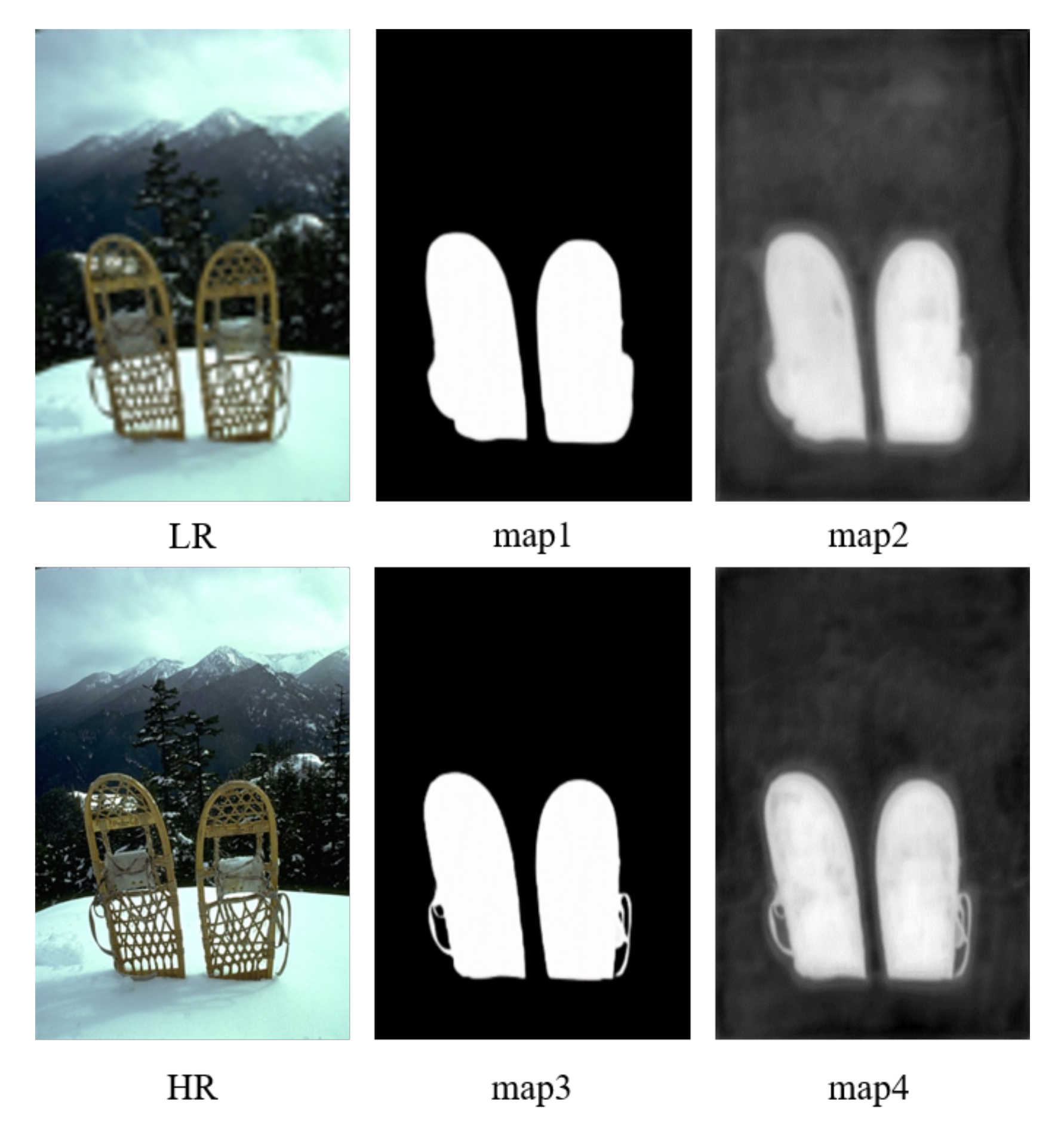
The saliency feature map reflects the saliency regions of the image and whether the image structure, texture, and other information are rich. We expect to capture more apparent differences among the saliency maps in our task. In Figure 7, we list a low-resolution image and a high-resolution image and their saliency maps before and after the Sigmoid layer, respectively. Map2 and map4 are the saliency diagrams of low-resolution and high-resolution images without the sigmoid layer. Map1 and map3 are the saliency diagrams through the sigmoid layer. Compared with map1 and map3, map2 and map4 show more apparent differences in target contour and deviation in the black-and-white degree. The output saliency maps from the Sigmoid layer (map1 and map3) are harder to distinguish in most areas. Therefore, to better utilize the difference between saliency maps and improve the super-resolution performance of remote sensing images, we choose the saliency feature maps before the Sigmoid layer. The saliency loss function is expressed in Equation (6).
where W and H represent the width and height of feature map, respectively. C indicates the number of feature channels. and are the extracted saliency maps from the target image and the generated image, respectively.
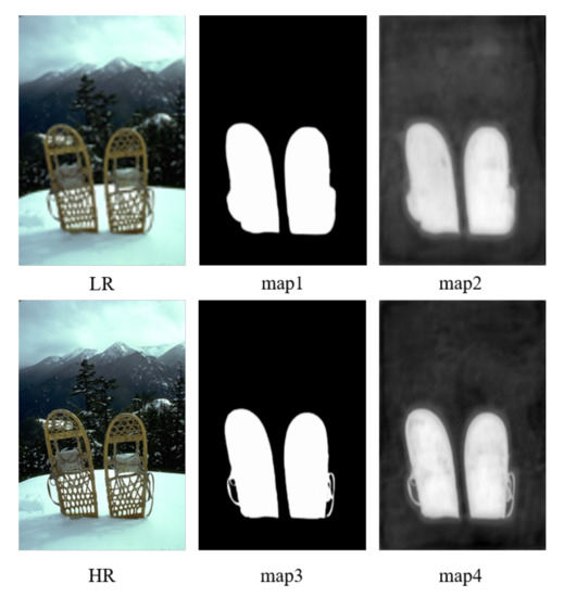
Figure 7.
Illustrate the LR and HR images and the corresponding saliency maps before (map2, map4) and after (map1, map3) Sigmoid layer.
3.4. Design of Basic Loss Functions
The saliency loss has been described in Section 3.3. This subsection mainly introduces the rest loss functions, including the loss, the perceptual loss, and the adversarial loss.
The loss is adopted to reduce the pixel-level differences, and the function is shown in Equation (7).
where C, W, and H represent the number of feature channels, the width, and the height of the feature map, respectively. represents the target remote sensing image, and is the generated remote sensing images.
The perceptual loss is the loss at the feature level, which focuses on considering image features. Besides, the perceptual loss utilizes the VGG network [50], which takes advantage of the high-level feature map. As the perceptual loss focuses on in-depth features, it can help improve the image’s clarity and achieve better visual effects. Equation (8) shows the formula of the loss.
where C, W, and H represent the number of feature channels, the width, and the height of feature map, respectively. indicates the feature extracted from the target image and is the feature extracted from generated image.
Adversarial loss is the basic loss of the generative adversarial network. The loss function contains the generator loss and the discriminator loss function. The details are shown in Equations (9) and (10).
here, and represent the adversarial loss of the generator and the adversarial loss of the discriminator, respectively. is the probability that the generated image is a generated remote sensing HR image, is the real remote sensing image and is the remote sensing LR image. Through the adjustment of these two loss functions, the continuous adjustment training between the generator and the discriminator is realized.
According to the experience [13] and parameter adjustment results, we set the weight for is , is , is 1.0, and is .
4. Experiments
In this section, we first introduce the training and testing dataset. Then we conduct experiments on test datasets. We use PSNR and SSIM as metrics to compare the SG-GAN algorithm quantitatively with existing advanced algorithms and show the visualization results.
4.1. Datasets and Metrics
SG-GAN is trained on RAISE [67] dataset, which contains a total of 8156 high-resolution images. We randomly flip and crop the images to make the training data more aplenty. The images are cropped into blocks as the high-resolution images. The corresponding low-resolution images are generated with the Bicubic method and clipped into blocks.
In testing stage, we test it on SR standard benchmarks, including Set5 [68], Set14 [69], BSD100 [70], and Urban100 [71]. In addition, to verify the advantages of salient object detection for SR, we also report the performance on MSRA10K [72], which is originally provided for the salient object annotation.
Moreover, to better evaluate the remote sensing image SR performance and generalization of the proposed SG-GAN, we randomly select images for five remote sensing datasets to evaluate our approach: NWPU VHR-10 datset [73], UCAS-AOD dataset [74], AID dataset [75], UC-Merced dataset [76], and NWPU45 dataset [77] according to categories, and then LR images obtained by bicubic downsampling to form remote sensing super-resolution datasets.
NWPU VHR-10 dataset [73]: This dataset consists of 800 images divided into 10 class geospatial objects, including airplanes, ships, storage tanks, baseball diamonds, tennis courts, basketball courts, ground track fields, harbors, bridges, and vehicles. We randomly select 10 images from each category, obtain LR images through bicubic downsampling, and use these 100 images as the test dataset.
UCAS-AOD dataset [74]: This dataset is designed for airplane and vehicle detection. Consisting of 600 images with 3210 airplanes and 310 images with 2819 vehicles. We randomly select 200 to obtain LR images through bicubic downsampling and use these images as the test dataset.
AID dataset [75]: This dataset consists of 10,000 images in 30 aerial scene categories, including airports, bare ground, baseball fields, beaches, bridges, centers, churches, commercials, dense residences, deserts, farmlands, forests, etc. The size of each image is pixels. We randomly select 10 images from each category, obtain LR images through bicubic downsampling and use these 300 images as the test dataset.
UC-Merced dataset [76]: This dataset consists of 2100 images in 21 land use categories, including agriculture, airplanes, baseball fields, beaches, buildings, small churches, etc. The size of each image is pixels. We randomly select 10 images from each category, obtain LR images through bicubic downsampling and use these 210 images as the test dataset.
NWPU45 dataset [77]: This dataset consists of 31,500 images of 45 scene categories, including airport, baseball diamond, basketball court, beach, bridge, chaparral, church, etc. The size of each image is pixels. We randomly select 10 images from each category, obtain LR images through bicubic downsampling and use these 450 images as the test dataset.
Following most remote sensing SR methods [1,78,79], the peak signal-to-noise ratio (PSNR) and structure similarity index (SSIM) are used to evaluate our model quantitatively. PSNR is formed as Equation (11), which measures the difference between corresponding pixels of the super-resolved image and the ground truth. SSIM is formed as Equation (12) and evaluates the structural similarity. Moreover, the performance of GAN-based methods (SRGAN, SRGAN + , and SG-GAN) are measured by additional indexes, including inception score (IS) [80], sliced Wasserstein distance (SWD) [81], and Frechet inception distance (FID) [82]. IS is given by Equation (13), which measures the diversity of generated images. FID compares the distributions of Inception embeddings of real and generated images as Equation (14). SWD approximates the Wasserstein-1 distance between the real and the generated images and calculates the statistical similarity between local image patches extracted from Laplacian pyramid representations.
where C, W, and H represent the number of feature channels, the width, and the height of the feature map, respectively. The refers to the mean square error between SR image x and remote sensing HR image y. represents the maximum signal value that exists in the HR image.
where , and , denote the mean and standard deviations of SR image (x) and remote sensing HR image (y), denotes the covariance of x and y, and and are used to refrain from dividing by zero.
where is a generated image sampled from the learned generator distribution , is the expectation over the set of the generated images, is the KL-distance between the conditional class distribution and the marginal class distribution .
where , denote the mean and covariance of the real and generated image distribution, respectively.
4.2. Implementation Details
In order to compare the improvement effect of our method with SRGAN, parameters and calculations of SG-GAN are set as almost or less than SRGAN. Therefore, the batch size is 16, and the training iteration epoch is 100. The optimization method we used is ADAM, and the and are and , respectively. We adopt the pre-trained saliency detection model BASNet, which is trained on the DUTS-TR [83] dataset. All the paper experiments were carried out using the Pytorch framework.
4.3. Comparison with the Advanced Methods
In this section, numerous experiments are described on the five SR datasets mentioned above. We compare our proposed method with various advanced SR methods, including Bicubic, FSRCNN [42], SRResnet [13], RCAN [46] and SRGAN [13].
Quantitative Results by PSNR/SSIM. Table 1 presents quantitative comparisons for SR. Compared with all the above approaches, our SG-GAN performs the best in almost all cases.

Table 1.
Evaluation results on the standard datasets. Red and blue indicate the best and second-best performance.
Qualitative Results. Figure 8 shows the qualitative results on SR standard benchmarks, and Figure 9 presents the visual results on the MSRA10K salient object database. We observe that most of the compared methods would suffer from blurring edges and noticeable artifacts, especially the saliency regions of the image. Compared with the interpolation method (Bicubic), the details of the image generated by the FSRCNN method are improved. However, the vision is still blurred, and insufficient edge information. With the deepening development of the network, the extracted deep features increase, SRResnet recovers more high-frequency information. RCAN subjoins the attention mechanism and obtains a better repair effect. Images generated by SRGAN get a tremendous visual impact, but many unreal details are also generated. In contrast, our SG-GAN gains much better results in recovering sharper and saliency areas, more faithful to the ground truth. These comparisons indicate that SG-GAN can better recover more salient and informative components in HR images and show competing image SR results than other methods.
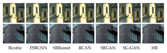
Figure 8.
Results of image super-resolution on the standard dataset using different algorithms.
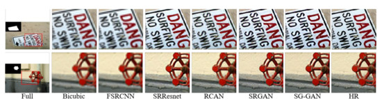
Figure 9.
Results of the different methods on the MSRA10K dataset mainly capture the saliency area of the images.
4.4. Application of Remote Sensing Image
Remote sensing images contain various objects and rich texture information. Therefore, the problem of super-resolution restoration of remote sensing images has always been a hotspot. To verify the performance of SG-GAN, we conducted experiments on five remote sensing datasets, which have been mentioned in Section 4.1.
Table 2 shows the quantitative results of scale factors . Among them, Bicubic, FSRCNN [42], SRResnet [13], RCAN [46], and SRGAN [13] are the advanced SR methods, and LGCNet [78], DMCN [1], DRSEN [79], DCM [84], and AMFFN [85] are remote sensing SR methods. The results of the advanced SR methods are tested with the pre-trained model of the DIV2K [86] dataset. For remote sensing SR methods, we directly use the results given in the original paper. Compared with the SRGAN, the PSNR of SG-GAN is improved +0.89 dB on the NWPU WHR-10 dataset, +1.53 dB on the UCAS-AOD dataset, +0.91 dB on the AID dataset, +1.85 dB on the UC-Merced dataset, and +0.98 dB on the NWPU45 dataset. The quantitative results demonstrated that SG-GAN utilizes the additional constraint to supervise the saliency map of the remote sensing images, which can obtain SR images with a higher quantitative index.
Table 2.
Evaluation results on remote sensing datasets. Red and blue indicate the best and second-best performance.
Furthermore, we test SRGAN, SRGAN + Lsa, and SG-GAN on IS, FID, and SWD to evaluate the performance of GAN-based networks. The results are shown in Table 3.
Table 3.
Generative quality evaluations of GAN-based SR methods on AID and UC-Merced. Red and blue indicate the best and second-best performance.
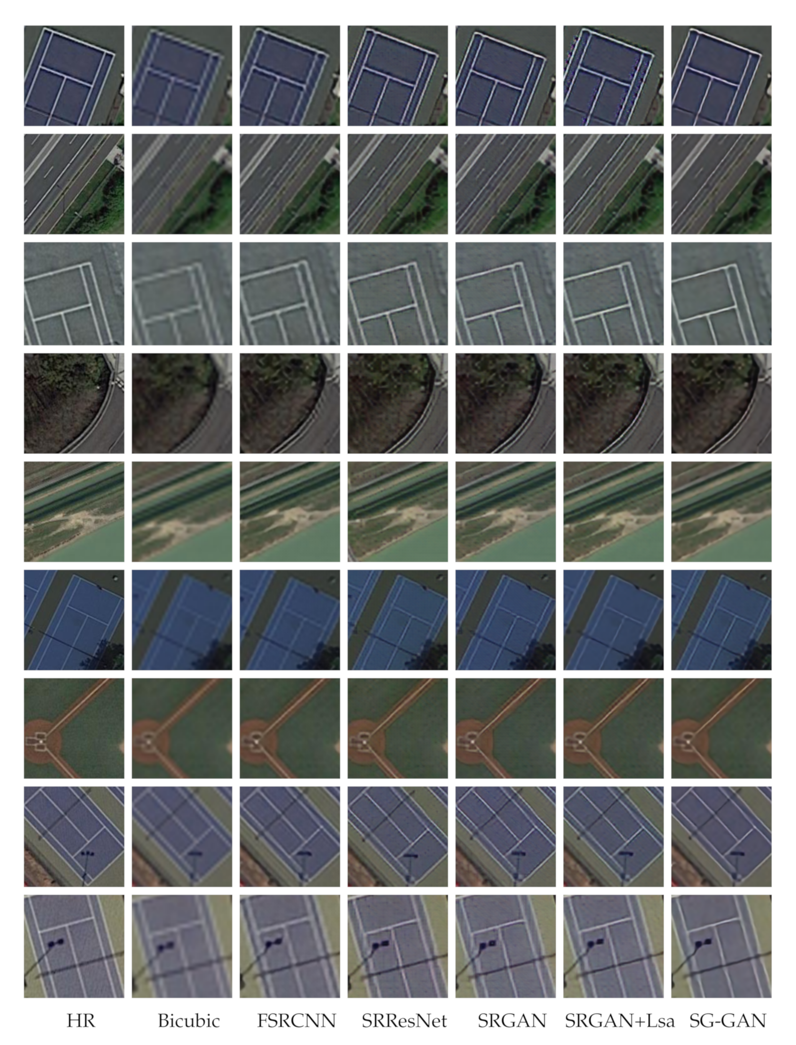
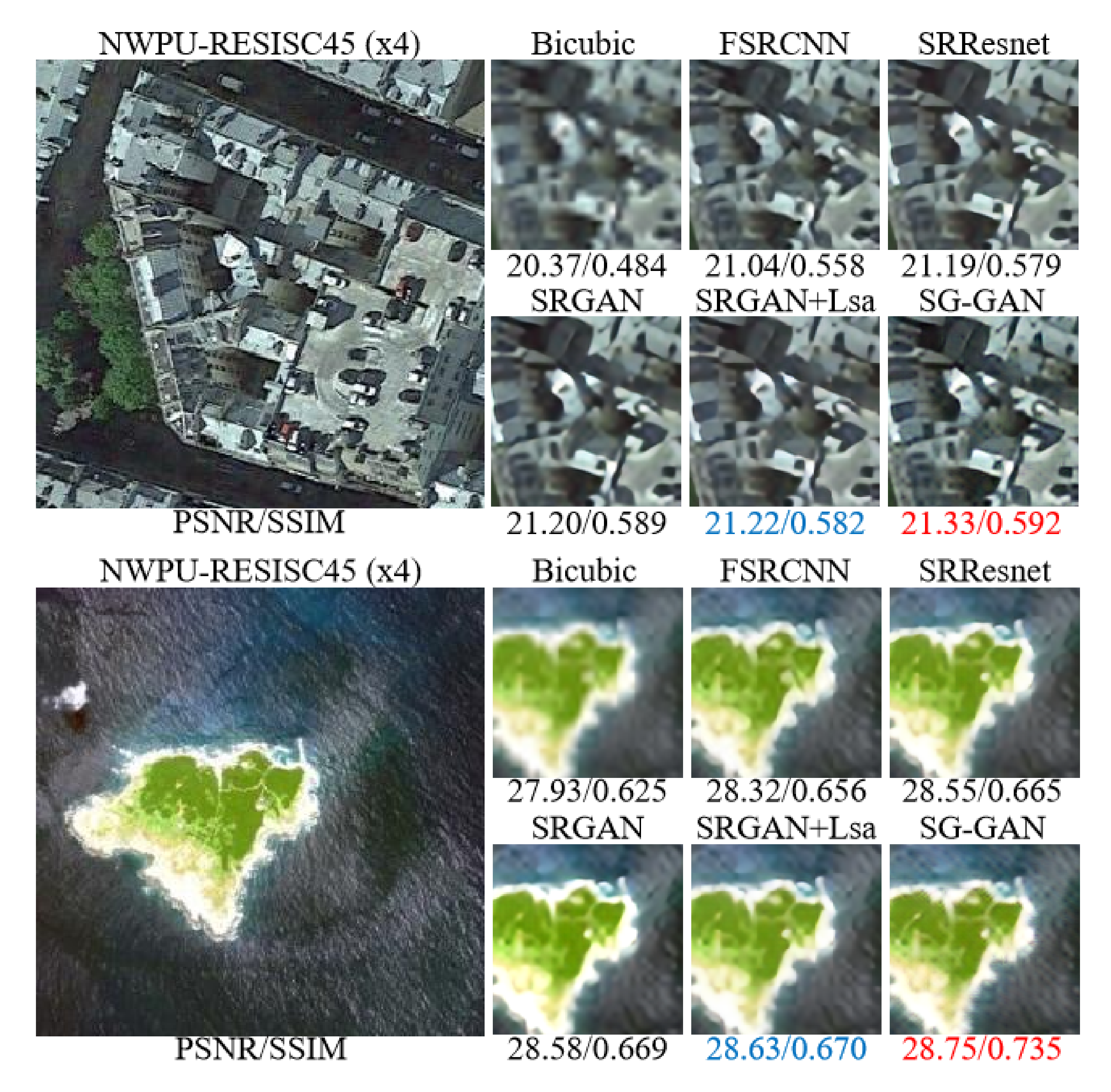
In order to fully demonstrate the effectiveness of SG-GAN, we present the SR visual results on UCAS-AOD dataset [74] in Figure 10, NWPU VHR-10 datset [73] in Figure 11, AID dataset [75] in Figure 12, UC-Merced dataset [76] in Figure 13, and NWPU45 dataset [77] in Figure 14.
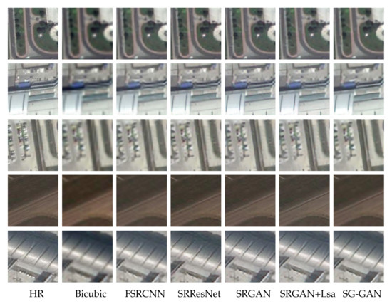
Figure 10.
Results on the UCAS-AOD dataset. Each row compares the results of images repaired by different methods; each column represents the repair results of different images under the same method.
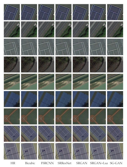
Figure 11.
Experiment results on the NWPU VHR-10 dataset. Each row compares the results of images repaired by different methods; each column represents the repair results of different images under the same method.
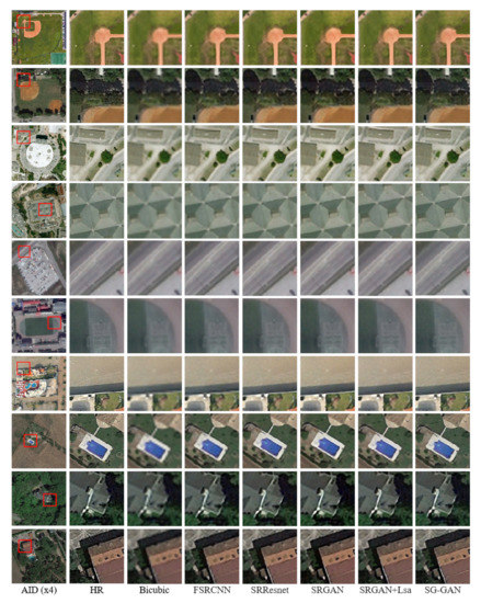
Figure 12.
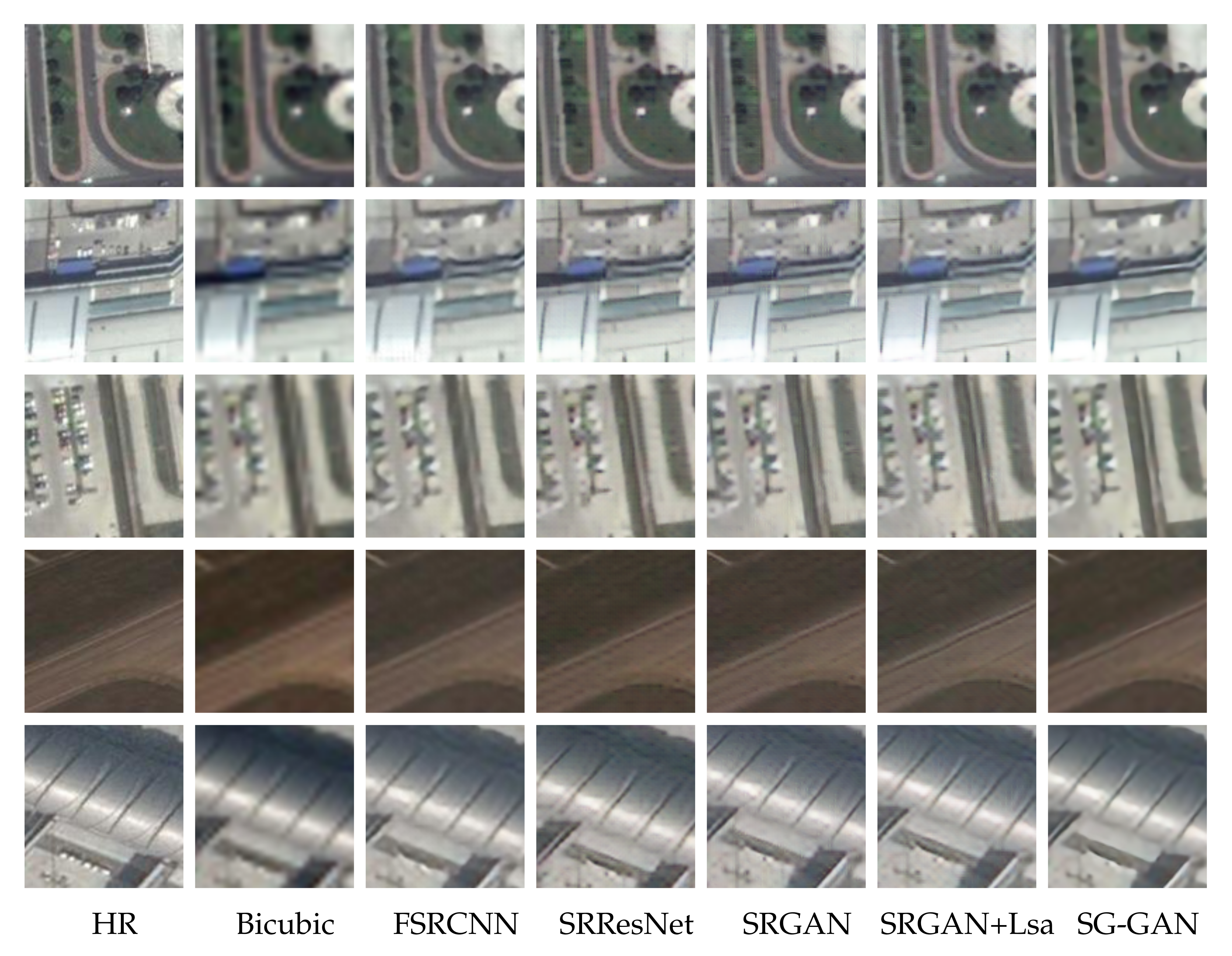
Qualitative comparison of scaling factors between SG-GAN and the advanced SR methods on AID dataset. Each row compares the results of images repaired by different methods; each column represents the repair results of different images under the same method.
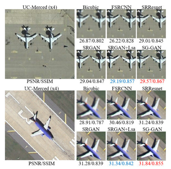
Figure 13.
Qualitative comparison of scaling factors between SG-GAN and advanced SR methods on UC-Merced dataset. The best result is in red and the second result is in blue.
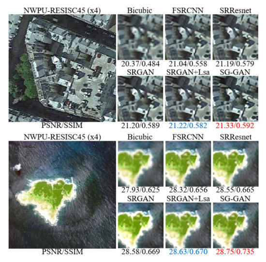
Figure 14.
Qualitative comparison of scaling factors between SG-GAN and advanced SR methods on NWPU-RESISC45 dataset. The best result is in red and the second result is in blue.
From what is demonstrated in qualitative results, the restoration difficulty of various parts is different. The non-saliency regions (e.g., ground, land, and lawn) are comparatively easier to super-resolution than the saliency regions as the latter have complex structures. The main difference among super-resolution methods is on saliency regions. Bicubic is a commonly used image interpolation method, which the surrounding pixel information is filled to obtain the pixel value through linear calculation. Therefore, the image obtained in this way will appear blurry. The other methods are based on deep learning, and their effects are better than interpolation-based methods.
FSRCNN is a relatively shallow network structure composed of various feature processing layers connected in series. Limited by the depth of the network, FSRCNN only learns more shallow feature information. When the reconstructed image is measured, the reconstructed image can obtain better PSNR and SSIM results. SRResnet deepens the network through residual connections. It can capture richer mid-frequency and high-frequency information, precisely what low-resolution images lack. Therefore, the reconstructed image quality will be significantly improved when the depth of the network increases.
SRGAN and SRResnet were proposed simultaneously, and the major-est difference between them is that SRGAN contains a discriminator. Although the discriminator will slow down the network training, adversarial training between the two networks can make the generator capture more feature information. However, the discriminator focuses on the mid-frequency and high-frequency image features, reducing the attention to the edge and color. Therefore, the generated image will have a particular deviation between the shallow feature information and the information of the actual value image.
The proposed SG-GAN motivates the network to focus on the salient features of the image, which helps the network pay attention to the complex area of the image so as to get a better-reconstructed image, which has the characteristic of reducing aliasing, blur artifacts, and better reconstructing high-fidelity details. From Figure 12, SG-GAN infers a sharp edge of the saliency area, indicating that our method is capable of capturing structural characteristics of objects in images. Our approach also recovers better textures than the compared SR methods in qualitative comparisons of other datasets. In other words, the structure and edge of the saliency region can benefit from the designed saliency loss. Although SG-GAN is also a generational adversarial structure, due to the efficient mining and utilization of features by the network, it makes up for the loss of shallow features. Experimental and visual results reflect the superiority of the SG-GAN algorithm.
4.5. Ablation Study
To validate our method further, we design an SRGAN + Lsa model, which adds the saliency loss reference in Equation (6) to the SRGAN model. Detailed ablation experiment results of quantitative results are in Table 2. After adding the loss in SRGAN, the PSNR of NWPU VHR-10, UCAS-AOD, AID, UC-Merced, and NWPU45 increase 0.85 dB, 0.56 dB, 0.55 dB, 1.36 dB, and 0.17 dB, respectively.
Figure 10, Figure 11, Figure 12, Figure 13 and Figure 14 have visualized the qualitative results on UCAS-AOD, NWPU VHR-10, AID, UC-Merced, and NWPU45 datasets, respectively. It is easier to distinguish the method’s pros and cons in the complex structure. The results show that the model’s experimental results with additional saliency loss are better than SRGAN. The salient discrepancies of each part of the image implicitly report the diversity in the image’s structure and features. Moreover, it gives extra care to more complex regions and plays a positive role in repairing a complete image. In other words, the saliency loss is helpful when dealing with the super-resolution problem of remote sensing images. It can pay more attention to the details of the edge and structure of the image and accurately depict the characteristics of the remote sensing image’s saliency area.
5. Discussion
Compared with SG-GAN, although the other advanced SR methods could generate more details and more explicit SR images, there are still existing edge distortions and wrong feature structures. This paper is demonstrated that the proper loss function is essential to improve the resolution results of remote sensing images SR. Several experiments have proved that increasing the attention to the salient part of remote sensing images can help restore the saliency region’s graph structures and enhance image SR performance.
However, our proposed methods demonstrate weaknesses in reconstructing arbitrary scale resolution. Only has favorable performance in remote sensing images super-resolution tasks with specific scale magnification (e.g., and ). Therefore, it is a future direction for our work to apply SR with more extensive and even arbitrary magnifications.
6. Conclusions
This paper proposes a saliency-guided remote sensing image super-resolution method (SG-GAN), which considers saliency differences in various regions of remote sensing images. As the structure of the saliency area of the image is more complex and the information contained is relatively affluent, increasing the attention to the saliency area is beneficial to the quality of the super-resolution image. Therefore, this paper utilizes the saliency target detection network to construct a saliency loss function to help the generator capture more helpful information. At the same time, the strategy of adversarial learning plays a crucial role in improving the ability of SG-GAN to grasp characteristic details.
This paper has conducted experiments on the saliency dataset, standard datasets, and remote sensing datasets, confirming that focusing more on the saliency area of the image is beneficial for improving the image’s resolution. Quantitative and qualitative experimental results have shown the effectiveness of the proposed method.
Author Contributions
Conceptualization, B.L., L.Z. and J.L.; methodology, B.L., L.Z., J.L. and W.C.; software, B.L., L.Z. and J.L.; validation, B.L., L.Z., J.L. and W.C.; formal analysis, B.L., L.Z. and J.L.; investigation, B.L., L.Z. and J.L.; resources, B.L., L.Z. and Y.W.; data curation, B.L., L.Z. and W.L.; writing—original draft preparation, L.Z.; writing—review and editing, B.L., L.Z., J.L., H.Z., W.L., Y.L., Y.W., H.C. and W.C.; visualization, L.Z.; supervision, B.L., L.Z., J.L., H.Z., W.L., Y.L., Y.W., H.C. and W.C.; project administration, B.L., W.L. and Y.W.; funding acquisition, B.L. and Y.W. All authors have read and agreed to the published version of the manuscript.
Funding
This research was supported by the Natural Science Foundation of Shandong Province under Grants ZR2019MF073, the Fundamental Research Funds for the Central Universities, China University of Petroleum (East China) under Grant 20CX05001A, the Major Scientific and Technological Projects of CNPC under Grant ZD2019-183-008, Creative Research Team of Young Scholars at Universities in Shandong Province under Grant 2019KJN019, and the National Natural Science Foundation of China under Grant 62072468.
Institutional Review Board Statement
Not applicable.
Informed Consent Statement
Not applicable.
Data Availability Statement
All data used and generated in this study are available for research purposes. Available online: https://github.com/upczhaolf/SG-GAN (accessed on 15 December 2021).
Acknowledgments
The authors would like to thank all colleagues in the laboratory for their generous help. The authors would like to thank the anonymous reviewers for their constructive and valuable suggestions.
Conflicts of Interest
The authors declare no conflict of interest.
Abbreviations
The following abbreviations are used in this manuscript:
| SG-GAN | saliency-guided remote sensing image super-resolution |
| HQ | high spatial quality |
| LQ | low spatial quality |
| SR | super-resolution |
| HR | high-resolution |
| LR | low-resolution |
| RB | residual blocks |
| CNN | convolutional neural network |
| GAN | generative adversarial network |
| FCN | fully connected neural network |
| SOD | salient object detection |
| BCE | binary cross-entropy |
| SSIM | structural similarity |
| IoU | intersection-over-Union |
| MSE | mean square error |
| PSNR | peak signal-to-noise ratio |
References
- Xu, W.; Xu, G.; Wang, Y.; Sun, X.; Lin, D.; Wu, Y. Deep memory connected neural network for optical remote sensing image restoration. Remote Sens. 2018, 10, 1893. [Google Scholar] [CrossRef] [Green Version]
- Clabaut, É.; Lemelin, M.; Germain, M.; Bouroubi, Y.; St-Pierre, T. Model Specialization for the Use of ESRGAN on Satellite and Airborne Imagery. Remote Sens. 2021, 13, 4044. [Google Scholar] [CrossRef]
- Allebach, J.; Wong, P.W. Edge-directed interpolation. In Proceedings of the 3rd IEEE International Conference on Image Processing, Lausanne, Switzerland, 19 September 1996; Volume 3, pp. 707–710. [Google Scholar]
- Freedman, G.; Fattal, R. Image and video upscaling from local self-examples. ACM Trans. Graph. (TOG) 2011, 30, 1–11. [Google Scholar] [CrossRef] [Green Version]
- Achanta, R.; Estrada, F.; Wils, P.; Süsstrunk, S. Salient region detection and segmentation. In Proceedings of the International Conference on Computer Vision Systems, Santorini, Greece, 12–15 May 2008; pp. 66–75. [Google Scholar]
- Shuai, L.; Yajie, Z.; Lei, X. Remote sensing image super-resolution method using sparse representation and classified texture patches. Geomat. Inf. Sci. Wuhan Univ. 2015, 40, 578–582. [Google Scholar]
- Yang, J.; Wright, J.; Huang, T.S.; Ma, Y. Image super-resolution via sparse representation. IEEE Trans. Image Process. 2010, 19, 2861–2873. [Google Scholar] [CrossRef]
- Dong, C.; Loy, C.C.; He, K.; Tang, X. Learning a deep convolutional network for image super-resolution. In Proceedings of the European Conference on Computer Vision, Zurich, Switzerland, 6–12 September 2014; pp. 184–199. [Google Scholar]
- Kim, J.; Kwon Lee, J.; Mu Lee, K. Accurate image super-resolution using very deep convolutional networks. In Proceedings of the IEEE Conference on Computer Vision and Pattern Recognition, Las Vegas, NV, USA, 27–30 June 2016; pp. 1646–1654. [Google Scholar]
- Zhang, Y.; Tian, Y.; Kong, Y.; Zhong, B.; Fu, Y. Residual dense network for image super-resolution. In Proceedings of the IEEE Conference on Computer Vision and Pattern Recognition, Salt Lake City, UT, USA, 18–23 June 2018; pp. 2472–2481. [Google Scholar]
- Goodfellow, I.; Pouget-Abadie, J.; Mirza, M.; Xu, B.; Warde-Farley, D.; Ozair, S.; Courville, A.; Bengio, Y. Generative adversarial nets. Adv. Neural Inf. Process. Syst. 2014, 2, 2672–2680. [Google Scholar]
- Johnson, J.; Alahi, A.; Fei-Fei, L. Perceptual losses for real-time style transfer and super-resolution. In Proceedings of the European Conference on Computer Vision, Amsterdam, The Netherlands, 8–16 October 2016; pp. 694–711. [Google Scholar]
- Ledig, C.; Theis, L.; Huszár, F.; Caballero, J.; Cunningham, A.; Acosta, A.; Aitken, A.; Tejani, A.; Totz, J.; Wang, Z.; et al. Photo-realistic single image super-resolution using a generative adversarial network. In Proceedings of the IEEE Conference on Computer Vision and Pattern Recognition, Honolulu, HI, USA, 21–26 July 2017; pp. 4681–4690. [Google Scholar]
- Sajjadi, M.S.; Scholkopf, B.; Hirsch, M. Enhancenet: Single image super-resolution through automated texture synthesis. In Proceedings of the IEEE International Conference on Computer Vision, Venice, Italy, 22–29 October 2017; pp. 4491–4500. [Google Scholar]
- Gatys, L.; Ecker, A.S.; Bethge, M. Texture synthesis using convolutional neural networks. Adv. Neural Inf. Process. Syst. 2015, 28, 262–270. [Google Scholar]
- Feng, X.; Zhang, W.; Su, X.; Xu, Z. Optical Remote Sensing Image Denoising and Super-Resolution Reconstructing Using Optimized Generative Network in Wavelet Transform Domain. Remote Sens. 2021, 13, 1858. [Google Scholar] [CrossRef]
- Bashir, S.M.A.; Wang, Y. Small Object Detection in Remote Sensing Images with Residual Feature Aggregation-Based Super-Resolution and Object Detector Network. Remote Sens. 2021, 13, 1854. [Google Scholar] [CrossRef]
- Kim, T.; Cha, M.; Kim, H.; Lee, J.K.; Kim, J. Learning to discover cross-domain relations with generative adversarial networks. In Proceedings of the 34th International Conference on Machine Learning, Sydney, Australia, 6–19 August 2017; PMLR. org. Volume 70, pp. 1857–1865. [Google Scholar]
- Huang, X.; Liu, M.Y.; Belongie, S.; Kautz, J. Multimodal unsupervised image-to-image translation. In Proceedings of the European Conference on Computer Vision (ECCV), Munich, Germany, 8–14 September 2018; pp. 172–189. [Google Scholar]
- Benaim, S.; Wolf, L. One-sided unsupervised domain mapping. In Proceedings of the Advances in Neural Information Processing Systems (NeurIPS), Long Beach, CA, USA, 4–9 December 2017; pp. 752–762. [Google Scholar]
- Zhu, H.; Peng, X.; Chandrasekhar, V.; Li, L.; Lim, J.H. DehazeGAN: When Image Dehazing Meets Differential Programming. In Proceedings of the International Joint Conferences on Artificial Intelligence (IJCAI), Stockholm, Sweden, 13–19 July 2018; pp. 1234–1240. [Google Scholar]
- Guo, J.; Liu, Y. Image completion using structure and texture GAN network. Neurocomputing 2019, 360, 75–84. [Google Scholar] [CrossRef]
- Guimaraes, G.L.; Sanchez-Lengeling, B.; Outeiral, C.; Farias, P.L.C.; Aspuru-Guzik, A. Objective-reinforced generative adversarial networks (ORGAN) for sequence generation models. arXiv 2017, arXiv:1705.10843. [Google Scholar]
- Abdollahi, A.; Pradhan, B.; Sharma, G.; Maulud, K.N.A.; Alamri, A. Improving Road Semantic Segmentation Using Generative Adversarial Network. IEEE Access 2021, 9, 64381–64392. [Google Scholar] [CrossRef]
- Tao, Y.; Xu, M.; Zhong, Y.; Cheng, Y. GAN-assisted two-stream neural network for high-resolution remote sensing image classification. Remote Sens. 2017, 9, 1328. [Google Scholar] [CrossRef] [Green Version]
- Jian, P.; Chen, K.; Cheng, W. GAN-Based One-Class Classification for Remote-Sensing Image Change Detection. IEEE Geosci. Remote. Sens. Lett. 2021, 1–5. [Google Scholar] [CrossRef]
- Wang, W.; Lai, Q.; Fu, H.; Shen, J.; Ling, H.; Yang, R. Salient object detection in the deep learning era: An in-depth survey. IEEE Trans. Pattern Anal. Mach. Intell. 2021. [Google Scholar] [CrossRef]
- Cong, R.; Lei, J.; Fu, H.; Cheng, M.M.; Lin, W.; Huang, Q. Review of visual saliency detection with comprehensive information. IEEE Trans. Circuits Syst. Video Technol. 2018, 29, 2941–2959. [Google Scholar] [CrossRef] [Green Version]
- Gao, Y.; Shi, M.; Tao, D.; Xu, C. Database saliency for fast image retrieval. IEEE Trans. Multimed. 2015, 17, 359–369. [Google Scholar] [CrossRef]
- Ma, C.; Miao, Z.; Zhang, X.P.; Li, M. A saliency prior context model for real-time object tracking. IEEE Trans. Multimed. 2017, 19, 2415–2424. [Google Scholar] [CrossRef]
- Zeng, Y.; Zhuge, Y.; Lu, H.; Zhang, L. Joint learning of saliency detection and weakly supervised semantic segmentation. In Proceedings of the IEEE/CVF International Conference on Computer Vision, Seoul, Korea, 27 October–2 November 2019; pp. 7223–7233. [Google Scholar]
- Fan, D.P.; Ji, G.P.; Zhou, T.; Chen, G.; Fu, H.; Shen, J.; Shao, L. Pranet: Parallel reverse attention network for polyp segmentation. In Proceedings of the International Conference on Medical Image Computing and Computer-Assisted Intervention, Lima, Peru, 4–8 October 2020; pp. 263–273. [Google Scholar]
- Fan, D.P.; Ji, G.P.; Sun, G.; Cheng, M.M.; Shen, J.; Shao, L. Camouflaged object detection. In Proceedings of the IEEE/CVF Conference on Computer Vision and Pattern Recognition, Seattle, WA, USA, 13–19 June 2020; pp. 2777–2787. [Google Scholar]
- Liu, Z.; Zhao, D.; Shi, Z.; Jiang, Z. Unsupervised saliency model with color Markov chain for oil tank detection. Remote Sens. 2019, 11, 1089. [Google Scholar] [CrossRef] [Green Version]
- Hou, B.; Wang, Y.; Liu, Q. A saliency guided semi-supervised building change detection method for high resolution remote sensing images. Sensors 2016, 16, 1377. [Google Scholar] [CrossRef] [Green Version]
- Zhang, L.; Liu, Y.; Zhang, J. Saliency detection based on self-adaptive multiple feature fusion for remote sensing images. Int. J. Remote Sens. 2019, 40, 8270–8297. [Google Scholar] [CrossRef]
- Cheng, M.M.; Mitra, N.J.; Huang, X.; Torr, P.H.; Hu, S.M. Global contrast based salient region detection. IEEE Trans. Pattern Anal. Mach. Intell. 2014, 37, 569–582. [Google Scholar] [CrossRef] [PubMed] [Green Version]
- Zhu, W.; Liang, S.; Wei, Y.; Sun, J. Saliency optimization from robust background detection. In Proceedings of the IEEE Conference on Computer Vision and Pattern Recognition, Columbus, OH, USA, 23–28 June 2014; pp. 2814–2821. [Google Scholar]
- Qin, X.; Fan, D.P.; Huang, C.; Diagne, C.; Zhang, Z.; Sant’Anna, A.C.; Suarez, A.; Jagersand, M.; Shao, L. Boundary-aware segmentation network for mobile and web applications. arXiv 2021, arXiv:2101.04704. [Google Scholar]
- Zhang, Z.; Lin, Z.; Xu, J.; Jin, W.D.; Lu, S.P.; Fan, D.P. Bilateral attention network for RGB-D salient object detection. IEEE Trans. Image Process. 2021, 30, 1949–1961. [Google Scholar] [CrossRef]
- Gao, S.H.; Tan, Y.Q.; Cheng, M.M.; Lu, C.; Chen, Y.; Yan, S. Highly efficient salient object detection with 100k parameters. In Proceedings of the European Conference on Computer Vision, Online, 23–28 August 2020; pp. 702–721. [Google Scholar]
- Dong, C.; Loy, C.C.; Tang, X. Accelerating the super-resolution convolutional neural network. In Proceedings of the European Conference on Computer Vision, Amsterdam, The Netherlands, 8–16 October 2016; pp. 391–407. [Google Scholar]
- Hui, Z.; Wang, X.; Gao, X. Fast and accurate single image super-resolution via information distillation network. In Proceedings of the IEEE Conference on Computer Vision and Pattern Recognition, Salt Lake City, UT, USA, 23–28 June 2018; pp. 723–731. [Google Scholar]
- Han, W.; Chang, S.; Liu, D.; Yu, M.; Witbrock, M.; Huang, T.S. Image super-resolution via dual-state recurrent networks. In Proceedings of the IEEE Conference on Computer Vision and Pattern Recognition, Salt Lake City, UT, USA, 23–28 June 2018; pp. 1654–1663. [Google Scholar]
- Li, J.; Fang, F.; Mei, K.; Zhang, G. Multi-scale residual network for image super-resolution. In Proceedings of the European Conference on Computer Vision (ECCV), Munich, Germany, 8–14 September 2018; pp. 517–532. [Google Scholar]
- Zhang, Y.; Li, K.; Li, K.; Wang, L.; Zhong, B.; Fu, Y. Image super-resolution using very deep residual channel attention networks. In Proceedings of the European Conference on Computer Vision (ECCV), Munich, Germany, 8–14 September 2018; pp. 286–301. [Google Scholar]
- Chen, W.; Zheng, X.; Lu, X. Hyperspectral Image Super-Resolution with Self-Supervised Spectral-Spatial Residual Network. Remote Sens. 2021, 13, 1260. [Google Scholar] [CrossRef]
- Huan, H.; Li, P.; Zou, N.; Wang, C.; Xie, Y.; Xie, Y.; Xu, D. End-to-End Super-Resolution for Remote-Sensing Images Using an Improved Multi-Scale Residual Network. Remote Sens. 2021, 13, 666. [Google Scholar] [CrossRef]
- He, K.; Zhang, X.; Ren, S.; Sun, J. Deep residual learning for image recognition. In Proceedings of the IEEE Conference on Computer Vision and Pattern Recognition, Las Vegas, NV, USA, 27–30 June 2016; pp. 770–778. [Google Scholar]
- Simonyan, K.; Zisserman, A. Very deep convolutional networks for large-scale image recognition. arXiv 2014, arXiv:1409.1556. [Google Scholar]
- Gong, Y.; Liao, P.; Zhang, X.; Zhang, L.; Chen, G.; Zhu, K.; Tan, X.; Lv, Z. Enlighten-GAN for Super Resolution Reconstruction in Mid-Resolution Remote Sensing Images. Remote Sens. 2021, 13, 1104. [Google Scholar] [CrossRef]
- Courtrai, L.; Pham, M.T.; Lefèvre, S. Small Object Detection in Remote Sensing Images Based on Super-Resolution with Auxiliary Generative Adversarial Networks. Remote Sens. 2020, 12, 3152. [Google Scholar] [CrossRef]
- Salgueiro Romero, L.; Marcello, J.; Vilaplana, V. Super-Resolution of Sentinel-2 Imagery Using Generative Adversarial Networks. Remote Sens. 2020, 12, 2424. [Google Scholar] [CrossRef]
- Gu, J.; Dong, C. Interpreting Super-Resolution Networks with Local Attribution Maps. In Proceedings of the IEEE/CVF Conference on Computer Vision and Pattern Recognition, Virtual, 19–25 June 2021; pp. 9199–9208. [Google Scholar]
- Romano, Y.; Isidoro, J.; Milanfar, P. RAISR: Rapid and accurate image super resolution. IEEE Trans. Comput. Imaging 2016, 3, 110–125. [Google Scholar] [CrossRef] [Green Version]
- Wang, X.; Yu, K.; Dong, C.; Loy, C.C. Recovering realistic texture in image super-resolution by deep spatial feature transform. In Proceedings of the IEEE Conference on Computer Vision and Pattern Recognition, Salt Lake City, UT, USA, 18–23 June 2018; pp. 606–615. [Google Scholar]
- Kong, X.; Zhao, H.; Qiao, Y.; Dong, C. ClassSR: A General Framework to Accelerate Super-Resolution Networks by Data Characteristic. In Proceedings of the IEEE/CVF Conference on Computer Vision and Pattern Recognition, Virtual, 19–25 June 2021; pp. 12016–12025. [Google Scholar]
- Zhao, R.; Ouyang, W.; Li, H.; Wang, X. Saliency detection by multi-context deep learning. In Proceedings of the IEEE Conference on Computer Vision and Pattern Recognition, Boston, MA, USA, 7–12 June 2015; pp. 1265–1274. [Google Scholar]
- Mahapatra, D.; Bozorgtabar, B. Retinal Vasculature Segmentation Using Local Saliency Maps and Generative Adversarial Networks For Image Super Resolution. arXiv 2017, arXiv:1710.04783. [Google Scholar]
- Qin, X.; Zhang, Z.; Huang, C.; Gao, C.; Dehghan, M.; Jagersand, M. BASNet: Boundary-Aware Salient Object Detection. In Proceedings of the IEEE Conference on Computer Vision and Pattern Recognition, Long Beach, CA, USA, 25–20 June 2019; pp. 7479–7489. [Google Scholar]
- He, K.; Zhang, X.; Ren, S.; Sun, J. Delving deep into rectifiers: Surpassing human-level performance on imagenet classification. In Proceedings of the IEEE International Conference on Computer Vision, Boston, MA, USA, 7–12 June 2015; pp. 1026–1034. [Google Scholar]
- Lim, B.; Son, S.; Kim, H.; Nah, S.; Mu Lee, K. Enhanced deep residual networks for single image super-resolution. In Proceedings of the IEEE Conference on Computer Vision and Pattern Recognition Workshops, Honolulu, HI, USA, 21–26 July 2017; pp. 136–144. [Google Scholar]
- De Boer, P.T.; Kroese, D.P.; Mannor, S.; Rubinstein, R.Y. A tutorial on the cross-entropy method. Ann. Oper. Res. 2005, 134, 19–67. [Google Scholar] [CrossRef]
- Wang, Z.; Simoncelli, E.P.; Bovik, A.C. Multiscale structural similarity for image quality assessment. In Proceedings of the Thrity-Seventh Asilomar Conference on Signals, Systems & Computers, Pacific Grove, CA, USA, 9–12 November 2003; Volume 2, pp. 1398–1402. [Google Scholar]
- Máttyus, G.; Luo, W.; Urtasun, R. Deeproadmapper: Extracting road topology from aerial images. In Proceedings of the IEEE International Conference on Computer Vision, Venice, Italy, 22–29 October 2017; pp. 3438–3446. [Google Scholar]
- Jaccard, P. The distribution of the flora in the alpine zone. 1. New Phytol. 1912, 11, 37–50. [Google Scholar] [CrossRef]
- Dang-Nguyen, D.T.; Pasquini, C.; Conotter, V.; Boato, G. Raise: A raw images dataset for digital image forensics. In Proceedings of the 6th ACM Multimedia Systems Conference, Portland, OR, USA, 18–20 March 2015; pp. 219–224. [Google Scholar]
- Bevilacqua, M.; Roumy, A.; Guillemot, C.; Alberi-Morel, M.L. Low-Complexity Single-Image Super-Resolution Based On Nonnegative Neighbor Embedding; British Machine Vision Conference (BMVC): Guildford, UK, 2012. [Google Scholar]
- Zeyde, R.; Elad, M.; Protter, M. On single image scale-up using sparse-representations. In Proceedings of the International Conference on Curves and Surfaces, Avignon, France, 24–30 June 2010; pp. 711–730. [Google Scholar]
- Martin, D.; Fowlkes, C.; Tal, D.; Malik, J. A database of human segmented natural images and its application to evaluating segmentation algorithms and measuring ecological statistics. In Proceedings of the Eighth IEEE International Conference on Computer Vision-ICCV 2001, Vancouver, BC, Canada, 7–14 July 2001; Volume 2, pp. 416–423. [Google Scholar]
- Huang, J.B.; Singh, A.; Ahuja, N. Single image super-resolution from transformed self-exemplars. In Proceedings of the IEEE Conference on Computer Vision and Pattern Recognition, Boston, MA, USA, 7–12 June 2015; pp. 5197–5206. [Google Scholar]
- Matsui, Y.; Ito, K.; Aramaki, Y.; Fujimoto, A.; Ogawa, T.; Yamasaki, T.; Aizawa, K. Sketch-based manga retrieval using manga109 dataset. Multimed. Tools Appl. 2017, 76, 21811–21838. [Google Scholar] [CrossRef] [Green Version]
- Cheng, G.; Han, J.; Zhou, P.; Guo, L. Multi-class geospatial object detection and geographic image classification based on collection of part detectors. ISPRS J. Photogramm. Remote Sens. 2014, 98, 119–132. [Google Scholar] [CrossRef]
- Xia, G.S.; Bai, X.; Ding, J.; Zhu, Z.; Belongie, S.; Luo, J.; Datcu, M.; Pelillo, M.; Zhang, L. DOTA: A large-scale dataset for object detection in aerial images. In Proceedings of the IEEE Conference on Computer Vision and Pattern Recognition, Salt Lake City, UT, USA, 18–23 June 2018; pp. 3974–3983. [Google Scholar]
- Xia, G.S.; Hu, J.; Hu, F.; Shi, B.; Bai, X.; Zhong, Y.; Zhang, L. AID: A benchmark data set for performance evaluation of aerial scene classification. IEEE Trans. Geosci. Remote Sens. 2017, 55, 3965–3981. [Google Scholar] [CrossRef] [Green Version]
- Yang, Y.; Newsam, S. Bag-of-visual-words and spatial extensions for land-use classification. In Proceedings of the 18th SIGSPATIAL International Conference on Advances in Geographic Information Systems, San Jose, CA, USA, 2–5 November 2010; pp. 270–279. [Google Scholar]
- Cheng, G.; Han, J.; Lu, X. Remote sensing image scene classification: Benchmark and state of the art. Proc. IEEE 2017, 105, 1865–1883. [Google Scholar] [CrossRef] [Green Version]
- Lei, S.; Shi, Z.; Zou, Z. Super-Resolution for Remote Sensing Images via Local–Global Combined Network. IEEE Geosci. Remote Sens. Lett. 2017, 14, 1243–1247. [Google Scholar] [CrossRef]
- Gu, J.; Sun, X.; Zhang, Y.; Fu, K.; Wang, L. Deep Residual Squeeze and Excitation Network for Remote Sensing Image Super-Resolution. Remote Sens. 2019, 11, 1817. [Google Scholar] [CrossRef] [Green Version]
- Salimans, T.; Goodfellow, I.; Zaremba, W.; Cheung, V.; Radford, A.; Chen, X. Improved techniques for training gans. Adv. Neural Inf. Process. Syst. 2016, 29, 2234–2242. [Google Scholar]
- Heusel, M.; Ramsauer, H.; Unterthiner, T.; Nessler, B.; Hochreiter, S. Gans trained by a two time-scale update rule converge to a local nash equilibrium. Adv. Neural Inf. Process. Syst. 2017, 30, 6629–6640. [Google Scholar]
- Karras, T.; Aila, T.; Laine, S.; Lehtinen, J. Progressive growing of gans for improved quality, stability, and variation. arXiv 2017, arXiv:1710.10196. [Google Scholar]
- Wang, L.; Lu, H.; Wang, Y.; Feng, M.; Wang, D.; Yin, B.; Ruan, X. Learning to detect salient objects with image-level supervision. In Proceedings of the IEEE Conference on Computer Vision and Pattern Recognition, Honolulu, HI, USA, 21–26 July 2017; pp. 136–145. [Google Scholar]
- Haut, J.M.; Paoletti, M.E.; Fernandez-Beltran, R.; Plaza, J.; Plaza, A.; Li, J. Remote Sensing Single-Image Superresolution Based on a Deep Compendium Model. IEEE Geosci. Remote Sens. Lett. 2019, 16, 1432–1436. [Google Scholar] [CrossRef]
- Wang, X.; Wu, Y.; Ming, Y.; Lv, H. Remote Sensing Imagery Super Resolution Based on Adaptive Multi-Scale Feature Fusion Network. Remote Sens. 2020, 20, 1142. [Google Scholar] [CrossRef] [Green Version]
- Agustsson, E.; Timofte, R. Ntire 2017 challenge on single image super-resolution: Dataset and study. In Proceedings of the IEEE Conference on Computer Vision and Pattern Recognition Workshops, Honolulu, HI, USA, 21–26 July 2017; pp. 126–135. [Google Scholar]


Publisher’s Note: MDPI stays neutral with regard to jurisdictional claims in published maps and institutional affiliations. |
© 2021 by the authors. Licensee MDPI, Basel, Switzerland. This article is an open access article distributed under the terms and conditions of the Creative Commons Attribution (CC BY) license (https://creativecommons.org/licenses/by/4.0/).