Abstract
It is very common to apply convolutional neural networks (CNNs) to synthetic aperture radar (SAR) automatic target recognition (ATR). However, most of the SAR ATR methods using CNN mainly use the image features of SAR images and make little use of the unique electromagnetic scattering characteristics of SAR images. For SAR images, attributed scattering centers (ASCs) reflect the electromagnetic scattering characteristics and the local structures of the target, which are useful for SAR ATR. Therefore, we propose a network to comprehensively use the image features and the features related to ASCs for improving the performance of SAR ATR. There are two branches in the proposed network, one extracts the more discriminative image features from the input SAR image; the other extracts physically meaningful features from the ASC schematic map that reflects the local structure of the target corresponding to each ASC. Finally, the high-level features obtained by the two branches are fused to recognize the target. The experimental results on the Moving and Stationary Target Acquisition and Recognition (MSTAR) dataset prove the capability of the SAR ATR method proposed in this letter.
1. Introduction
Synthetic Aperture Radar (SAR) can realize high-resolution microwave imaging through the synthetic aperture principle. Because of the high resolution, the capability of being free from the influence of weather and illumination, and the effectiveness of distinguishing camouflage and penetrating coverings, SAR is better than other remote sensing methods in many applications both in military and civil fields. Therefore, it has attracted increasing attention during the past years. However, compared with optical images, the unique speckle noise and different imaging mechanism in SAR images make the interpretation of SAR images more difficult [1]. Automatic target recognition (ATR) is one of the pivotal steps of SAR images interpretation and has great significance in both civil and military fields [2].
With the emergence of extensive data sets and the growth of computer processing power, deep learning has been widely used in many fields. In order to imitate the human brain’s cognitive mechanism, deep learning constructs a multi-level model structure to achieve multi-layer nonlinear transformation, through which the original data can be mapped into a feature space more suitable for recognition. Convolutional neural network (CNN) is a typical network used in image classification, which achieves feature extraction and classification using a unified framework and can automatically learn features more suitable for classification. Several existing studies [3] show that the deep features learned through convolution operations inclined to be more discriminatory for different types of targets. Currently, there are many SAR ATR methods based on CNN. Chen et al. [1] constructed a new network called A-ConvNet for SAR ATR, which has no fully connected layers and only contains convolution layers. The method in [1] can settle the over-fitting problem of CNN caused by insufficient training data to a certain extent. Leonan et al. [4] recognized oil rigs from Sentinel-1 SAR images using VGG-16 and VGG-19. Huang et al. [5] proposed a lightweight CNN for SAR ATR, which has global stream and local stream. The two streams are used to extract multi-level features, which will be combined to classify the target.
Although the CNN-based methods for SAR ATR have achieved good results, most of them mainly use the image information of SAR images and make little use of the unique electromagnetic scattering characteristics of SAR images. For SAR images, attributed scattering centers (ASCs) can use several physically relevant parameters to accurately describe the electromagnetic scattering characteristics and the local structures of the target, which are notably effective for SAR ATR [6]. At present, some ASC-based methods for SAR ATR have been proposed. Based on the Bayesian theory, Chiang et al. [7] proposed an ASC matching method, which evaluates the similarity between two ASC sets by the posterior probability. Dungan et al. [8] calculated the distance between the attributed point set of the test image and the attributed point sets of training samples using the least trimmed square Hausdorff distance (LTS-HD). The category of the test image is determined through the shortest distance. Tian et al. [9] also proposed an ASC matching method, which calculates the correspondence between test ASC set and template ASC sets to recognize the test image.
The abovementioned ASC-based methods for SAR ATR are based on ASC matching. Considering the powerful performance of CNN on SAR ATR, there have been some attempts to combine the ASCs of SAR targets and CNN to achieve SAR ATR. Lv et al. [10] extracted ASCs from the SAR image first, and then used different numbers of ASCs to obtain the reconstructed SAR images. The training set is augmented by these reconstructed SAR images. This method only uses the ASC reconstructed images to augment the training samples, which does not really realize the combination of ASC and CNN. Jiang et al. [11] fused the CNN and ASC matching hierarchically to achieve SAR ATR. In this hierarchical fusion method, CNN is used to classify the test sample first, and its output is used to calculate a reliability level. Then, the reliability level is used to judge whether the ASC matching need to be used to further classify the test sample. This method divides the whole recognition process into two separated stages, which is not an end-to-end network architecture and cannot be jointly optimized.
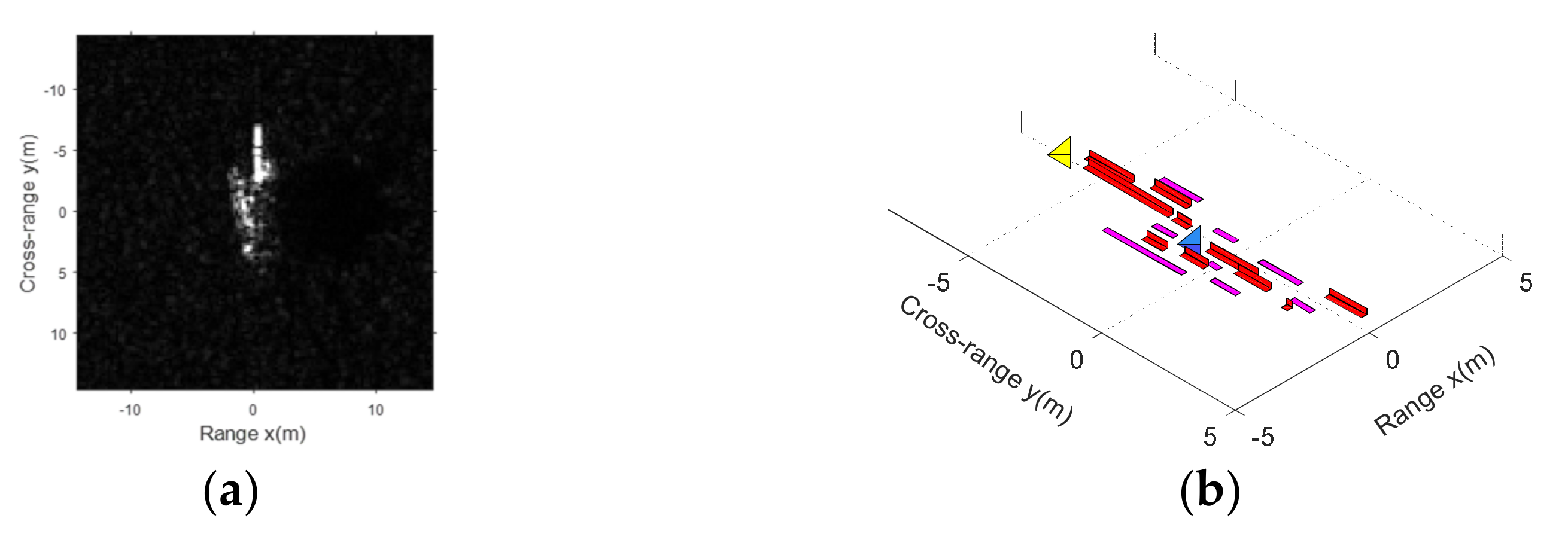
In order to combine the ASCs of SAR targets and CNN to achieve an end-to-end network structure, the ASC schematic map obtained through the physically relevant parameters of ASCs is adopted as one of the inputs of CNN in our method. As shown in Figure 1b, the ASC schematic map contains the geometric shape of each ASC extracted from the SAR image, such as dihedral, trihedral and so on. The ASC schematic map mainly describes the scattering centers of the target in the SAR image. There is no background clutter, and the target is composed of scattered geometric structures. Since the ASC schematic map can reflect the local structure of the target corresponding to each ASC, it is also meaningful for SAR ATR.

Figure 1.
The SAR image and the ASC schematic map of a T72 tank: (a) The SAR image of T72; (b) The ASC schematic map of T72.
In this paper, we propose a CNN combined with ASCs for SAR ATR to comprehensively utilize the features related to SAR images and the features related to ASCs, which can improve the accuracy of SAR ATR. There are two branches in the proposed network. The input of one branch is SAR image, more discriminative image features of which can be extracted in this branch. The input of the other branch is the ASC schematic map generated via the ASC model, which reflects the local structure of the target corresponding to each ASC, and features with physical meaning can be extracted in this branch. Since the two branches can complement each other, we fuse the high-level features obtained by the two branches to recognize the target. The whole network is jointly optimized.
2. Proposed Target Recognition Method
Figure 2 shows the overall framework of our method. It can be seen from Figure 2 that our proposed method contains two separated feature extraction networks, one feature fusion part and a classification part. Both feature extraction networks are composed of some convolutional layers and a fully-connected layer. In the two branches, one takes the SAR image obtained through executing a modulo operation on original complex SAR data as input, more discriminative image features of which can be extracted in this branch. The SAR image only contains the amplitude information of the complex SAR data. The other takes the corresponding ASC schematic map, which is obtained via the ASC model from the complex SAR data, as input and this branch can acquire features related to the target’s local structures. The ASC schematic map contains the amplitude information and phase information of the complex SAR data. These two types of features are complementary to each other. Therefore, the features obtained from the above-mentioned two branches are input into the feature fusion part. The feature fusion part contains a feature concatenation layer and a fully-connected layer with 1024 units. The fused feature obtained from the feature fusion part contains richer information of the SAR target, which are more descriptive and more discriminative. Finally, the fused feature is delivered into the classification part, which contains a fully-connected layer and a softmax function. The fully-connected layer in the classification part is used to reduce the dimensionality of the fused feature, and the number of units in this layer is equal to the number of categories. The softmax function is used to determine the target label. The output of the softmax function is a vector, where the value represents the probability that the input image belongs to each category. The target label will be determined as the class with the maximum probability. During the network training, the entire network is trained with the cross-entropy loss function, and two branches are jointly optimized.
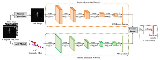
Figure 2.
The overall framework of our method, in which “conv” represents the convolution operation and “fc” indicates the fully connected operation. The parameters of the convolution operation are represented as “(number of convolution kernels) @ (filter size)”.
2.1. Attributed Scattering Center Model
For a distributed target in high frequency region, it can be seen as a composition of several independent scattering centers. Therefore, we can summate the responses of these scattering centers to approximate the radar backscattering of the distributed target as follows [12]:
where indicates the frequency; means the aspect angle; means the number of target’s ASC; indicates the ASCs’ parameter set. For a single ASC, the ASC model can be used to describe its backscattering field as follows [12]:
where indicates the propagation velocity of the electromagnetic wave; means radar center frequency; for the th ASC, means the complex amplitude; means the frequency dependence; the position coordinates of a scattering center in the range dimension and azimuth dimension are shown by and , respectively; the orientation and length of a distributed ASC are shown by and , respectively; the aspect dependence of a localized ASC is .
2.2. The ASC Schematic Map
For a distributed target in high frequency region, the dependence of its backscattering response on azimuth and frequency can be described through a set of parameters of the ASC model. These parameters can describe the physical characteristics of scattering centers in the target, including relative amplitude, shape, position and orientation (pose) [12]. Among these parameters, two of them are selected to differentiate eight iconic shapes of ASCs, which are listed in Table 1. Different colors are used to illustrate these eight shapes. As we can see in Table 1, the length of the edge broadside and edge diffraction cannot be distinguished by only the Length () but can be distinguished by combining both Frequency Dependence () and Length (); therefore, they are denoted in different colors in Table 1.

Table 1.
Shapes inference from frequency dependence and length [13].
It is a high-dimensional, non-linear and non-convex problem to estimate ASC parameters. Currently, there are many methods based on image domain processing or frequency domain processing for estimating ASC parameters. Most existing estimation methods in image domain rely on the image segmentation to estimate the parameters of ASC [14], the estimation results of which highly depend on the accuracy of the image segmentation. Compared with the estimation methods in image domain, there is no need to segment image in the estimation methods in frequency domain. However, the high computational complexity and storage demand of the estimation methods in frequency domain also limit their applications.
Since we use the ASC schematic map as the input of one of the network branches, an accurate ASC schematic map is of great significance for the final recognition result. In order to obtain accurate ASC schematic map, we adopt the method in [13] to extract ASCs of the input image. The method in [13] is a new ASC extraction algorithm in image domain, which has a good accuracy and a fast calculation speed. In this method, SAR measurements are converted to the sparse representations in image domain first. Then, the ASC model parameters are estimated through the Newtonized orthogonal matching pursuit (NOMP) algorithm. Specifically, there are four iterative steps in the ASCs extraction algorithm in [13], namely, atom selection, atom refinement, projection, and residue evaluation. Therefore, a signal can be sparsely approximated through a set of refined atoms. Detailed operations of this algorithm are summarized as Algorithm 1.
After obtaining parameters of all ASCs extracted from the input SAR image, the geometric shape of each ASC can be determined according to the frequency dependence parameter and length parameter, and then according to the position parameters of all ASCs, the ASC schematic map of the input SAR image can be obtained. The obtained ASC schematic map reflects the local structure of the target corresponding to each ASC and will be used as the input of the ASC schematic map branch. Figure 1 gives an example of the SAR image and its corresponding ASC schematic map.
| Algorithm 1 The ASCs extraction algorithm proposed in [13] |
|
| Output: |
| Initialization: residual image |
while the stop criterion is not met. do
|
| end while |
2.3. Feature Extraction Networks
CNN is one of the representative algorithms of deep learning, which has been widely used in image interpretation. Due to its deep architecture, CNN can automatically integrate the extracted features into abstract features layer by layer, and the obtained features are more applicable for classification. In our network, there are two feature extraction networks. The inputs of these two branches are different, one is SAR image, and the other is ASC schematic map. Therefore, it is reasonable to design different architectures for these two feature extraction networks. For the SAR branch, we consider the following aspects to design the feature extraction network:
- (1)
- In CNN, the extracted features of higher layer contain richer semantic information and tend to have better ability to distinguish different types of targets. However, the deeper the network, the larger the number of parameters, and larger amounts of labeled data are needed to estimate the parameters. In real scenarios, it is very difficult and costly to collect large amounts of labeled SAR images. Therefore, considering the feature extraction ability and parameter quantity of the network, we built a simple and efficient CNN architecture as the feature extraction network, which has 5 convolutional layers and one fully-connected layer.
- (2)
- According to existing experience, the number of convolution kernels is generally increased layer by layer. For SAR branch, we hope this branch can extract features that are more descriptive and more discriminative from the input SAR image. Therefore, we set a larger number of convolution kernels in each layer to learn better features, which are 96, 96, 512, 512, 1000, and 1000, respectively.
- (3)
- In CNN, the larger the convolution kernel, the larger the receptive field. And in SAR images, large receptive fields can alleviate the effect of speckle noise by degrees. In addition, the receptive fields of the shallower layers are relatively small while those of deeper layers are relatively large in CNN. Considering that large convolution kernels introduce large parameters, we reduce the sizes of the convolution kernels in our feature extraction network layer by layer, which are , , , , and , respectively.
For the ASC branch, we consider the following aspects to design the feature extraction network:
- (1)
- Compared with SAR image, ASC schematic map is easier. It should be more reasonable that the architecture of the ASC branch is simpler than SAR branch. Therefore, we decrease the number of convolutional kernels of each layer in the ASC branch to make it simpler, which are 16, 32, 64, 128, and 256, respectively.
- (2)
- There is almost no noise in the ASC schematic map. Therefore, the ASC branch does not require large-sized convolution kernels like SAR branch. And we just select convolution kernels with the size of 5 × 5 and 3 × 3.
- (3)
- In CNN, the receptive fields of the shallower layers are relatively small while those of deeper layers are relatively large. In addition, considering that large convolution kernels introduce large parameters, thus, 5 × 5 convolution kernels are applied in the first two layers to increase receptive field considerably and reduce the size of feature maps rapidly. 3 × 3 convolution kernels are utilized in the other layers.
The two feature extraction network architectures in our proposed method are different but each one is combined with convolutional layers, pooling layers and fully connected layer. Following each convolutional layer, there is a batch normalization (BN) layer, which can speed up the convergence of the network, prevent gradient explosion and gradient disappearance, and prevent overfitting [15]. After each convolution layer and BN layer, a max pooling is performed with a kernel size of 3 × 3 and a stride of 2 pixels. After the five convolutional layers, a fully connected layer is used to transform feature maps to a feature vector. The number of units in this layer is 1024. All activation functions used in the feature extraction networks are the rectified linear unit (ReLU).
During the training of our designed network, the weights are initialized from Gaussian distributions with zero mean and a standard deviation of 0.01, and biases are initialized with a constant value of 1. In many existing networks, the initial learning rate is mostly set to 0.001, 0.01 or 0.1. Considering that a too large learning rate may cause the model to fail to converge, while a too small learning rate will cause the model to converge slowly, the learning rate in our network is initially 0.01. The update rule of the learning rate is to reduce the learning rate when the loss of the network becomes stable. In our paper, the learning rate decreases by a factor of 0.1 after 15,000 iterations. Considering the computer’s memory and computing power, the batch size is set to be 16. And the max iteration is set to be 80,000 to ensure complete convergence of the network.
Through the two feature extraction networks, the information contained in SAR image and ASC schematic map can be learned, respectively. The deep network structure can map the shallow features into high-level abstract features layer by layer. The final feature vectors obtained by the feature extraction networks are more suitable for recognition.
3. Experimental Results
3.1. Data Description
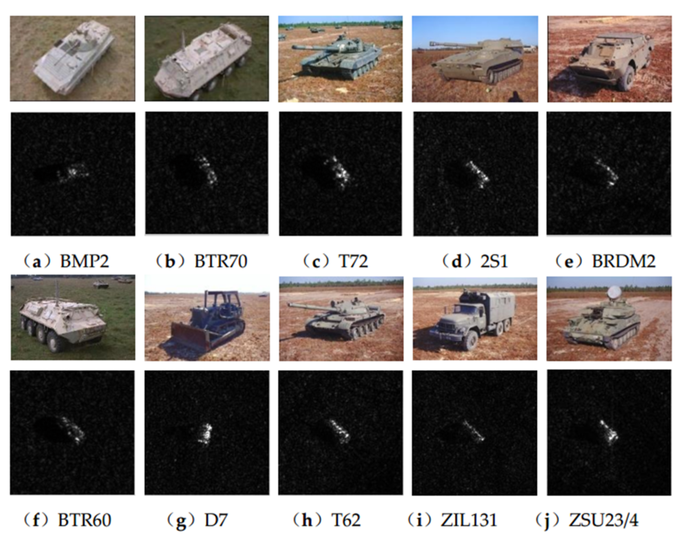
In this letter, the MSTAR dataset [16], which includes ten different types of ground targets, is used in experiments. Images in this dataset are collected through the X-band SAR sensor in m resolution. Some examples of these ten types of ground targets are shown as Figure 3, including optical images and corresponding SAR images.
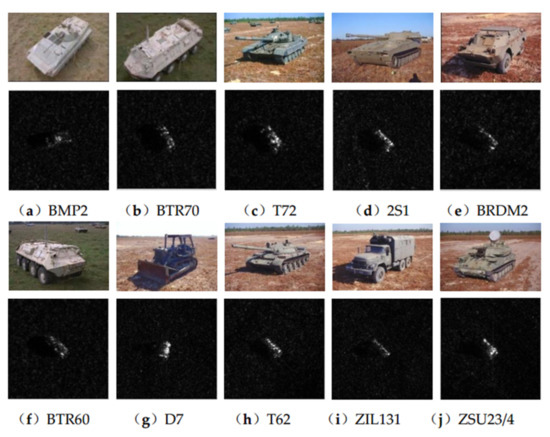
Figure 3.
Examples of ten types of ground targets. Optical images are on the top and SAR images are on the bottom.
The MSTAR dataset includes two widely used experimental settings, i.e., the three-target data and ten-target dada. There are three types of targets in the three-target data, in which T72 and BMP2 are two types of tanks and BTR70 is one type of armored vehicle. Each target has aspect angles ranging from to , and depression angles at 15° and 17°. Table 2 lists the specific information of the three-target data. There are three different serial numbers in BMP2 and T72. In detail, for each type, the training data only has one serial number, whereas the test data has all serial numbers. Additionally, we use images with 17° depression angle as training data, and images with 15° depression angle as test data.
Table 2.
The detailed information of training and test samples in three-target MSTAR data.
The ten-target data contain the data from ten different types of ground targets. Table 3 lists the specific information of the ten-target data. For each type, the training data only has one serial number, whereas the test data has all serial numbers. Additionally, we also use images with 17° depression angle as training data, and images with 15° depression angle as test data. Our network and experiments are implemented using the Caffe [17] framework under Ubuntu 16.04 Linux system.
Table 3.
The detailed information of training and test samples in ten-target MSTAR data.
3.2. Comparison Experiments with Several SAR ATR Methods
In this subsection, we use several methods for SAR ATR as the references to prove the capability of our method. The A-ConvNet [1] and Vgg-16 [18] are two CNN-based methods for SAR ATR with good performance, and both methods augment the training data. Actually, methods based on data augmentation have some problems in practical applications, such as how many times the data should be augmented and how to select suitable augmentation ways for each method and so on. In contrast, all these problems do not exist in our proposed method because there is no need to augment the training data in our proposed method. Therefore, for purpose of ensuring fairness, comparison experiments are conducted based on the parameters and network structure supplied in references [1] and [18] without data augmentation. The “ASC1” represents the method in [8], which calculates the distance between two ASC sets using the LTS-HD. The “ASC2” represents the method in [9], which calculates the one-to-one correspondence between test ASC set and template ASC sets to recognize the test image. The “Hierarchical fusion” represents the method in [11], which fuse the CNN and ASC matching hierarchically to achieve SAR ATR. Considering that the inputs of the above-mentioned methods are different, some are only related to SAR images, some are only related to ASCs of targets, and some are related to both SAR images and ASCs of targets. We divide all referenced methods and our method into three types: SAR-based methods, ASC-based methods, and fusion-based methods. SAR-based methods include A-ConvNet, Vgg-16, and the SAR branch in our proposed network. ASC-based methods include ASC1, ASC2, and the ASC branch in our proposed network. Fusion-based methods include hierarchical fusion and our proposed network. We compare our proposed method with the above-mentioned SAR ATR methods using the three-target data and ten-target data, respectively. The comparison results are shown by the accuracy rate measured in terms of the following equation [19]:
As can be seen, it is the ratio of the correct number predicted to the total number in the sample sets. In addition, considering the influence of the random initialization of the weights, we did 5 repeated experiments for each method. And the highest result of the 5 repeated experiments is used to represent the final accuracy.
3.2.1. The Three-Class Experiments
The dataset used in the three-class experiment is the three-target data listed in Table 2. Table 4 gives the Accuracies of all methods. It can be seen from Table 4 that the Accuracy of our proposed method is 0.9795, which is higher than that of A-ConvNet and Vgg-16. The reason is that CNN-based methods cannot work well with insufficient training samples. In the three-target data, for each type, the training data only has one serial number, whereas the test data has all serial numbers. This data setting makes the performance of A-ConvNet and Vgg-16 worse than the proposed method. In addition, the proposed method also has a higher Accuracy than ASC1 and ASC2, the reason is that our proposed method uses the information not only from the SAR image but also from the corresponding ASC schematic map. The results of the three-class experiment not only prove the effectiveness of the SAR ATR method proposed in this letter, but also indicate that our method can better make use of ASCs and SAR image to improve the recognition performance.
Table 4.
Recognition performance of several SAR target recognition methods on three-target MSTAR data.
3.2.2. The Ten-Class Experiments
The proposed method is further evaluated on ten-target data. The dataset used in the ten-class experiment is the ten-target data listed in Table 3. Table 5 gives the Accuracies of all methods. In Table 5, the Accuracy of the proposed method on ten-target data is 0.9869, which is higher than all other compared methods. The results further confirm that our method can still work better with increasing target types.
Table 5.
Recognition performance of several SAR target recognition methods on ten-target MSTAR data.
It can be seen from Table 4 and Table 5, for SAR-based methods, the A-ConvNet and VGG16 are less accurate than SAR branch in our proposed method. Compared with the A-ConvNet, the SAR branch in our proposed method has more convolution kernels with different sizes. Therefore, the SAR branch in our proposed method can learn better feature representations for the input than A-ConvNet, which makes the SAR branch in our proposed method perform better than A-ConvNet. Compared with VGG16, the SAR branch in our proposed method is a small network with less parameters, which is more suitable for the MSTAR dataset with insufficient labeled training samples. Therefore, the SAR branch in our proposed method performs better on the MSTAR dataset than VGG16. It can be also seen from Table 4 and Table 5, for ASC-based methods, results of the ASC branch in our proposed method are less accurate than all other ASC results. The “ASC1” and “ASC2” in Table 4 and Table 5 are both based on ASC template matching, utilizing the parameters of ASC that contain rich information of the target. Compared with them, the input of the ASC branch in our proposed method is the ASC schematic map obtained by the parameters of ASC. However, since not all the ASC parameters are used to generate the ASC schematic map, the information contained in the ASC schematic map is less than that in ASC parameters, which results in the worse performance of the ASC branch in our proposed method than ASC1 and ASC2 in Table 4 and Table 5. Although the performance of the ASC-based methods in Table 4 and Table 5 is better, they are very complicated. Compared with them, the ASC branch in our proposed method is simpler and easier to achieve. For fusion-based methods, our proposed method is more accurate than hierarchical fusion. The reason is that hierarchical fusion method uses the reliability level calculated by the outputs of CNN to judge whether the ASC matching need to be used to further classify the test sample, the accuracy of which highly depends on the results of CNN. However, the CNN used in the hierarchical fusion method is relatively simple, which may lead to poor recognition results, so that the misclassified test samples cannot be all selected by the calculated reliability level. Our proposed method comprehensively uses the image information and the local structure information of the SAR target, which can provide richer information for classification and obtain better accuracy. In addition, our proposed method performs better than all other methods in Table 4 and Table 5. The results also show that a single SAR branch or ASC branch may not achieve the best performance, but comprehensively using the two types of information can achieve the best performance, which proves the effectiveness of the combination of these two types of information.
3.3. Visualization of Ablation Experiments
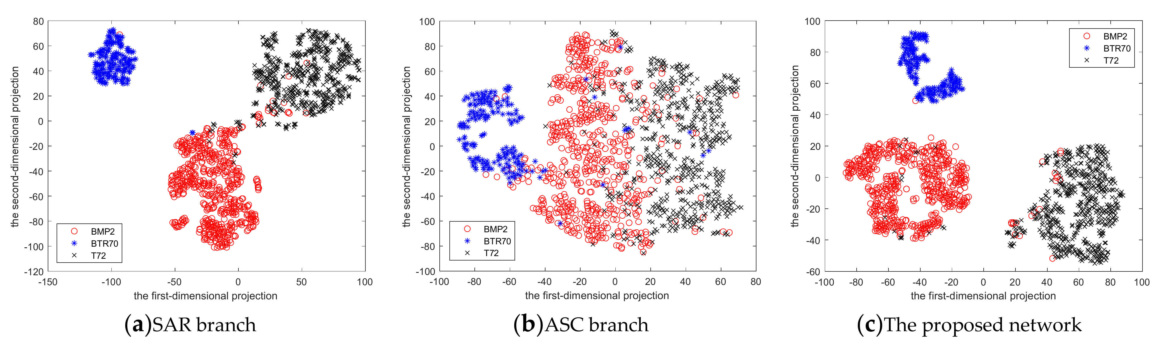
Table 4 and Table 5 has proved the effectiveness of comprehensively using the image information and the local structure information of the SAR target. In order to show this effectiveness more intuitively, we take the feature vectors obtained by the SAR branch, the ASC branch and the proposed network as high-dimensional features, and the distribution of these features will be visualized by the t-SNE algorithm [20]. The t-SNE algorithm is a commonly used nonlinear dimensionality reduction method, which is very suitable for reducing the dimensionality of high-dimensional data to two or three dimensions for visualization. This technique for the visualization of similarity data can retain the local structure of the data while also reveal some important global structure (such as clusters at multiple scales). Figure 4 shows the distribution of high-dimensional features extracted by the three networks, where each color represents a type of target.
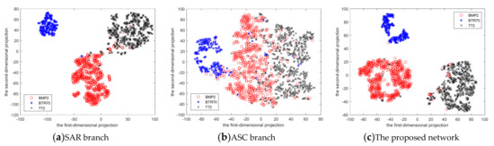
Figure 4.
t-SNE visualizations of the learned features. (a), (b), and (c) are the learned features corresponding to the SAR network, ASC network and the proposed network, respectively.
From Figure 4, we can see that compared with the high-dimensional features obtained by the SAR branch and the ASC branch, the high-dimensional feature extracted by the proposed network is more separable, and the boundaries between various features are more obvious, which can qualitatively prove the effectiveness of comprehensively using the image information of the SAR target and the local structure information of the SAR target. In addition, it can be seen from Figure 4c, for the test data, there are many positive recognitions and some negative recognitions in our method. Some examples of the positive and negative recognition in our experiments are shown as Figure 5.


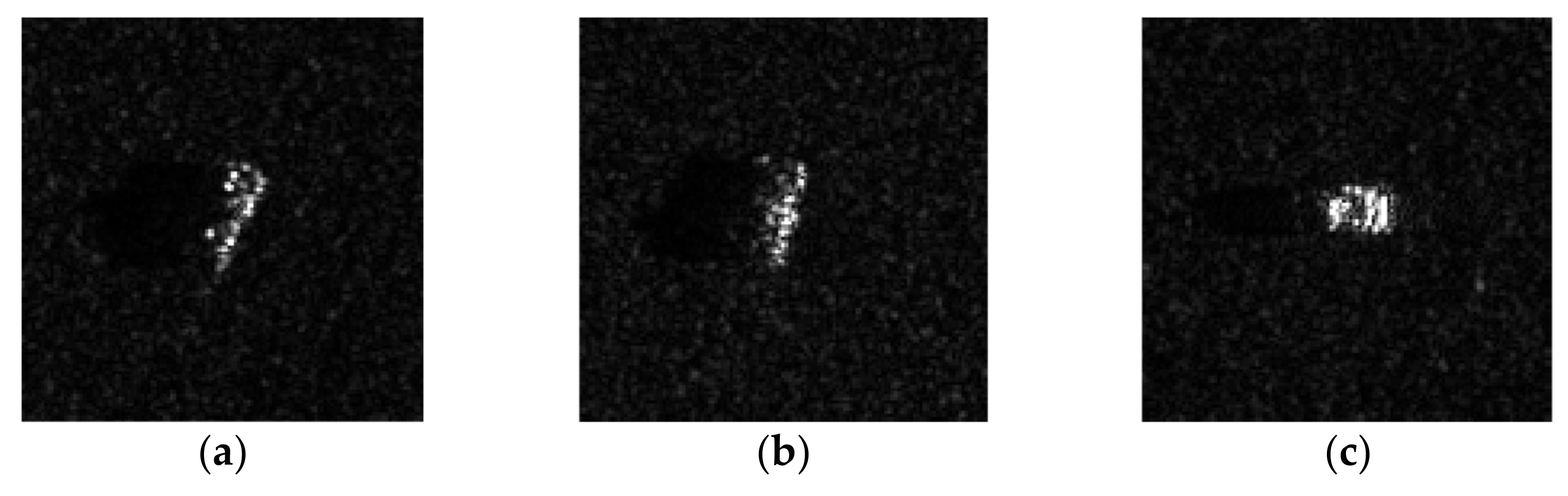
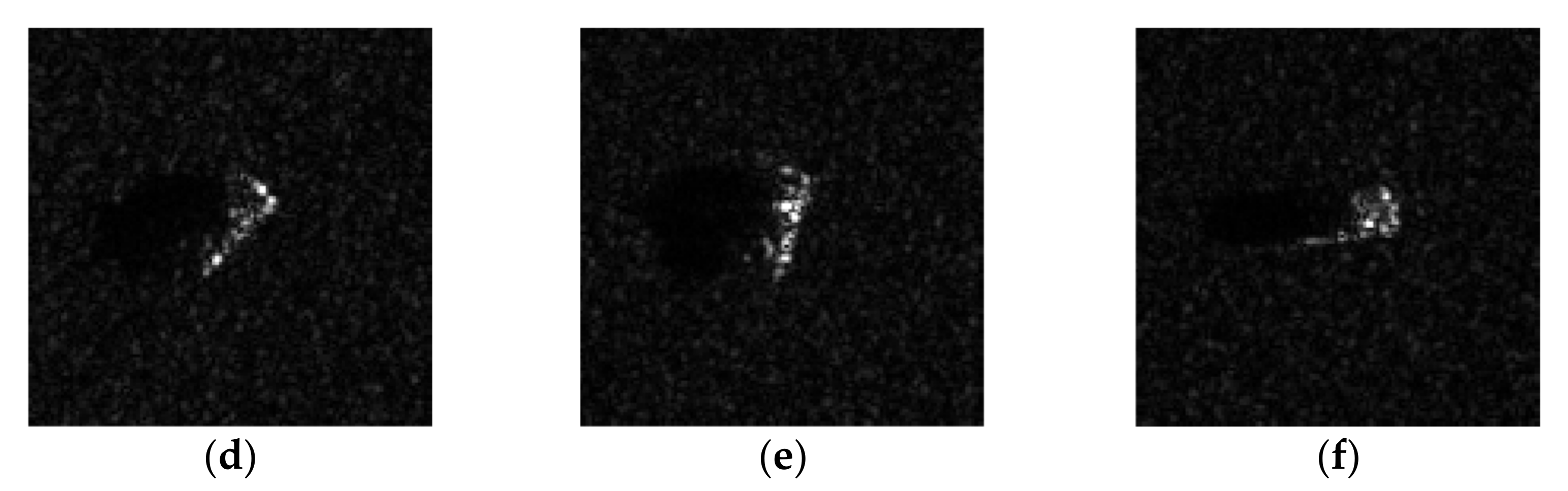
Figure 5.
Some examples of the positive and negative recognition of our method. (a) An example of positive recognition for BMP2. (b) An example of positive recognition for BTR70. (c) An example of positive recognition for T72. (d) An example of negative recognition for BMP2. (e) An example of negative recognition for BTR70. (f) An example of negative recognition for T72.
Figure 5a–c show three examples of positive recognition of our method, and d–f present three examples of negative recognition of our method. Compared with the positive recognition examples in a–c, the target intensities in the negative recognition examples in d–f are relatively weak. In addition, the missing parts of the targets in d–f are more serious than those in a–c. Therefore, compared with the samples of positive recognition, the samples of negative recognition are more difficult to be classified correctly.
3.4. Computational Complexity Analysis
According to the calculation principle of CNN [21], the computational complexity of all convolutional layers in the network is , where denotes the total number of convolutional layers in the network, represents the current convolutional layer’s index, for layer, and are the number of channels in input and output feature maps, represents the kernel size, and denotes the size of the output feature maps. The computational complexity of all fully connected layers in the network is , where represents the total number of fully connected layers in the network, represents the current fully connected layer’s index, for layer, and are the number of input and output nodes. According to the reference [14], the computational complexity of the ASC extraction in our method is , where denotes the number of significant ASCs extracted from the input image, and are the number of discrete levels for and , represents the size of the input SAR image, is the accuracy requirement of Newton’s method, and represents the complexity for an -dimensional cluster containing atoms.
In our proposed method, the overall computational complexity can be divided into four parts: the computational complexity of the SAR image branch, the computational complexity of the ASC schematic map branch, the computational complexity of feature fusion, and the computational complexity of classification. Based on the above analysis, the complexity formulas of the four parts are shown in Table 6. Their detailed floating-point operations (FLOPs) are related to the size of the input image and the number of ASCs extracted from the complex SAR data. For example, if the size of the input SAR image is 128 × 128 × 1, the size of the input ASC schematic map is 128 × 128 × 3, and the number of ASCs extracted from the complex SAR data is 15, then the FLOPs of each part based on the specific architecture of the proposed network are shown in Table 6.
Table 6.
Computational complexity of the proposed method.
From Table 6, we can see that the main part of the computational complexity in our method is from the two branches. For SAR image branch, the network architecture is complex, which results in large FLOPs. For ASC schematic map branch, there are two parts, which are ASCs extraction and feature extraction through network. The number of FLOPs of ASCs extraction is comparable to that of the SAR image branch, which cannot be ignored. In addition, although the network architecture of ASC schematic map branch is simple, compared with the SAR image branch, the input of the feature extraction network in this branch is the ASC schematic map, which is the colorful image and has three channels. Therefore, the FLOPs of feature extraction through network in this branch is also cannot be ignored. However, the two branches of the network are independent, which can be processed in parallel during execution. This parallel operation enables our method to have a comparable computational speed with the single-branch network method.
4. Discussion
The experimental results in Section 3 indicate that our proposed method improves recognition performance. For example, on the three-target MSTAR data, our method outperforms the A-ConvNet and VGG-16 in terms of accuracy by 4.1% and 3.74%, respectively. In addition, our method outperforms the ASC matching based methods in terms of accuracy by at least 1.61% and outperforms the hierarchical fusion of CNN and ASC matching in terms of accuracy by 3.0%. Moreover, on the more complicated ten-target MSTAR data, our method also outperforms all other comparison methods in terms of accuracy by at least 6.46%. A few discussions on our method are given as follows.
4.1. Cross Validation
Cross validation is the usual experimental setup in machine learning. The problem when test data is used to fit hyperparameters of the model, it is likely to overfit to that test data with bad generalization performance in new data. Cross validation would allow to evaluate dependence of the model on the train/test split as also the stability of the model. It is also the best way to fit hyperparameters. In order to evaluate the stability of our proposed method and demonstrate the effectiveness of ASC features, we perform the cross validation of our proposed method and SAR branch using the ten-target MSTAR data in Table 3. Firstly, we divide each type of training data in Table 3 into five equal portions. Then, four portions are selected from each type of training data to form a new training set, and the remaining one of each type is used to form a validation set. In this way, five different training-validation sets can be obtained. Next, we use each training set to train the network separately and use the trained network to recognize the corresponding validation set to obtain the network with optimal parameters on each validation set. Finally, the recognition results of the five optimal networks on the test data in Table 3 are shown in Table 7.
Table 7.
The recognition results of the cross validation using the ten-target MSTAR data.
In Table 7, the numbers 1 to 5 represent experiments using five different training-validation sets; “mean ± std” means the mean value and the standard deviation value of accuracies obtained from five cross-validation experiments; “All training data” represents using all training data in Table 3 to train the network. Some conclusions can be drawn from Table 7. Firstly, the validation set comes from the training data in Table 3. Therefore, when the amount of training data is insufficient, the accuracy of cross validation is lower than that of training the network using all the training data both for proposed method and SAR branch. Secondly, the standard deviation values of proposed method and SAR branch are 0.0024 and 0.0025, respectively. The relatively small standard deviation values indicate the low dependence of the proposed method and SAR branch on the train/test split as also the high stability of the model. Finally, the accuracy difference between the proposed method and SAR branch is 1.97%. And the mean value difference of cross validation between the proposed method and SAR branch is 2.06%. These results indicate that the accuracy difference is not an effect of the train/test split but an effect of using ASC features, which effectively demonstrate the effectiveness of ASC features in our proposed method.
4.2. Occlusion Situation
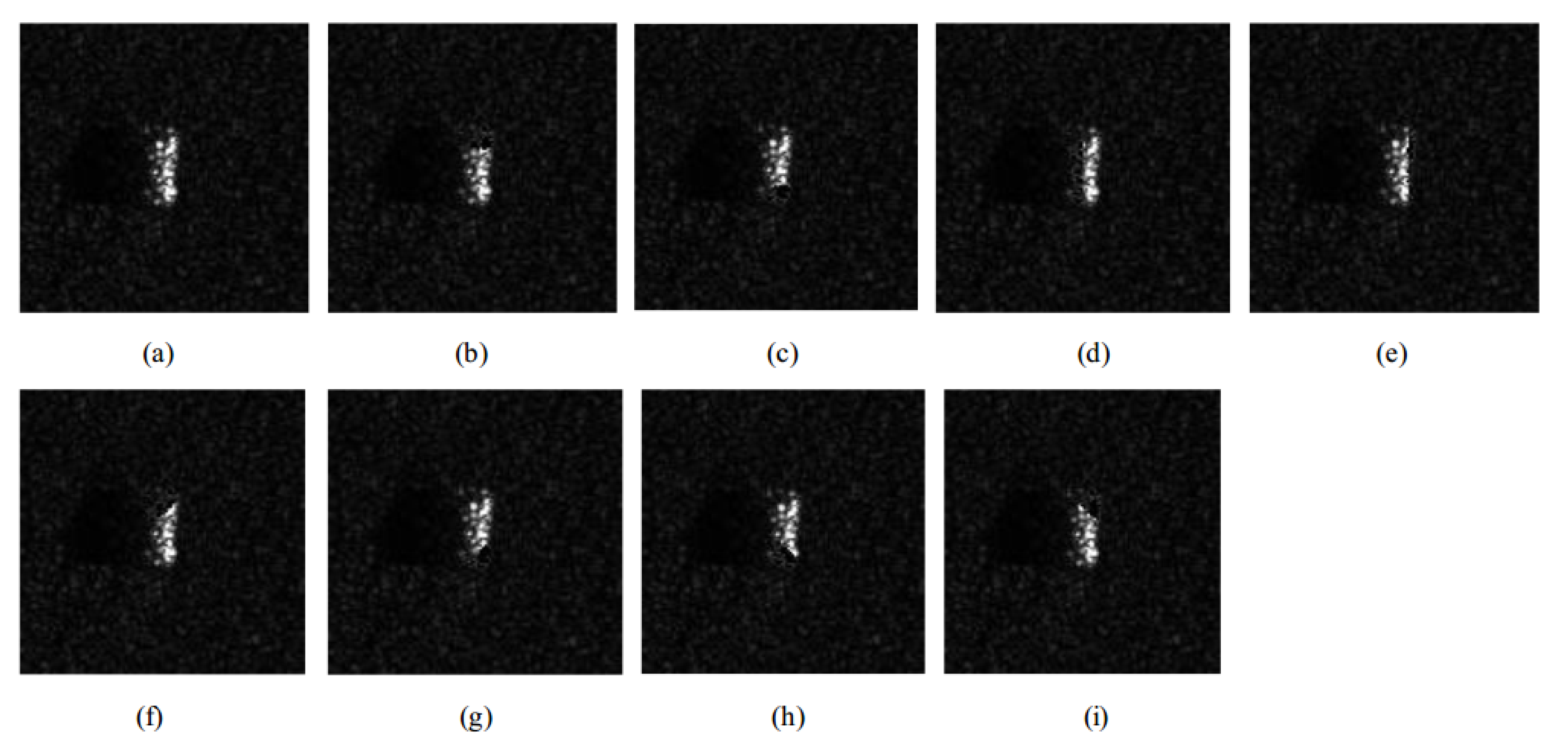
The dataset used in our paper is MSTAR dataset, which is a widely used SAR target recognition dataset in many existing works [1,2,5,10,11,22,23,24]. However, the real scenarios may be more complicated, such as the target is partially occluded by other objects. In order to validate the performance of our method in more complicated scenarios, we use the MSTAR three-target data to simulate the scenarios with occlusions. The target may be occluded by the obstacles or camouflaged intentionally. In this case, part of the target may not appear in the captured SAR image. On the basis of the SAR occlusion model in [2,25], we simulate the partially occluded image through removing a certain proportion of the target region in the original image from eight directions. Figure 6 shows SAR images with 20% occlusion from eight different directions.

Figure 6.
20% occluded images from different directions. (a) Original image; (b) direction 1; (c) direction 2; (d) direction 3; (e) direction 4; (f) direction 5; (g) direction 6; (h) direction 7; (i) direction 8.
In order to further prove the effectiveness of our method under more complex terrain with occlusions, we only occlude the test data while the training data remains unchanged. Table 8 shows the Accuracies of the test images which are occluded 20% from four different directions while the remaining ones are in the symmetrical directions.
Table 8.
Accuracies of four different occluded directions.
It can be seen from Table 8, the accuracy of each occluded direction is about 90% and the average Accuracy of these four different occluded directions is 90.66%, which proves that our method is still effective even when the test data is occluded and the test data contains variants that are not in the training data.
From the simulated occluded experiment, we can conclude that our method can not only used for MSTAR dataset, but also generalize to other SAR ATR datasets. However, our method cannot used for optical dataset. Because the input of the ASC branch in our method is related to the electromagnetic scattering characteristic of the target, which is the special characteristic in the SAR image and does not exist in optical image.
5. Conclusions
CNNs have excellent feature self-learning ability and have been widely used in many fields. However, many existing CNNs have large number of parameters, which need to be learned by larger amounts of labeled data. Actually, it is very difficult and costly to collect large amounts of labeled SAR images in real scenarios. Therefore, we construct a simple and efficient CNN architecture as the feature extraction network, which has fewer parameters that need to be learned while still having better feature learning ability than some existing networks, such as A-ConvNet and VGG-16. In addition, although several different kinds of CNNs have been applied to SAR ATR and achieved good results, most of them mainly use the image information of SAR targets and make little use of the unique electromagnetic scattering characteristics of SAR targets. For SAR targets, ASCs can use several physically relevant parameters to accurately describe the electromagnetic scattering characteristics and the local structures of the target, which are notably effective for SAR ATR. Therefore, we propose a network to comprehensively use the image information contained in SAR image and the local structure information contained in ASCs for improving the performance of SAR ATR. The experiments on real SAR dataset show that comprehensively using the two types of information can achieve the best performance than all compared methods, which proves the effectiveness of the combination of these two types of information.
Author Contributions
The idea of this method was proposed by Y.L. and W.X., and the experiments were also performed by them. Y.Z. provided many useful suggestions for this method. L.L. provided some useful suggestions for the writing. Y.L. wrote this manuscript. All authors have read and agreed to the published version of the manuscript.
Funding
This work was partially funded by the National Science Foundation of China, grant number 61871305.
Institutional Review Board Statement
Not applicable.
Informed Consent Statement
Not applicable.
Data Availability Statement
Not applicable.
Conflicts of Interest
The authors declare there is no conflict of interest.
References
- Chen, S.; Wang, H.; Xu, F.; Jin, Y. Target classification using the deep convolutional networks for SAR images. IEEE Trans. Geosci. Remote. Sens. 2016, 54, 4806–4817. [Google Scholar] [CrossRef]
- Ding, B.; Wen, G. Exploiting Multi-View SAR Images for Robust Target Recognition. Remote. Sens. 2017, 9, 1150. [Google Scholar] [CrossRef] [Green Version]
- Krizhevsky, A.; Sutskever, I.; Hinton, G.E. Imagenet classification with deep convolutional neural networks. In Proceedings of the Neural Information Processing System (NIPS), Harrahs and Harveys, Lake Tahoe, NV, USA, 3–8 December 2012; Volume 2, pp. 1096–1105. [Google Scholar]
- Falqueto, L.E.; Sá, J.A.; Paes, R.L.; Passaro, A. Oil Rig Recognition Using Convolutional Neural Network on Sentinel-1 SAR Images. IEEE Geosci. Remote. Sens. Lett. 2019, 16, 1329–1333. [Google Scholar] [CrossRef]
- Huang, X.; Yang, Q.; Qiao, H. Lightweight Two-Stream Convolutional Neural Network for SAR Target Recognition. IEEE Geosci. Remote. Sens. Lett. 2020, 99, 667–671. [Google Scholar] [CrossRef]
- Potter, L.C.; Moses, R.L. Attributed scattering centers for SAR ATR. IEEE Trans. Image Process. 1997, 6, 79–91. [Google Scholar] [CrossRef] [PubMed] [Green Version]
- Chiang, H.; Moses, R.L.; Potter, L.C. Model-based classification of radar images. IEEE Trans. Inf. Theory 2000, 46, 1842–1854. [Google Scholar] [CrossRef]
- Dungan, K.E.; Potter, L.C. Classifying transformation-variant attributed point patterns. Pattern Recognit. 2010, 43, 3805–3816. [Google Scholar] [CrossRef]
- Tian, S.; Yin, K.; Wang, C.; Zhang, H. An SAR ATR method based on scattering center feature and bipartite graph matching. IETE Tech. Rev. 2015, 32, 364–375. [Google Scholar] [CrossRef]
- Lv, J.; Liu, Y. Data augmentation based on attributed scattering centers to train robust CNN for SAR ATR. IEEE Access 2019, 7, 25459–25473. [Google Scholar] [CrossRef]
- Jiang, C.; Zhou, Y. Hierarchical Fusion of Convolutional Neural Networks and Attributed Scattering Centers with Application to Robust SAR ATR. Remote. Sens. 2018, 10, 819. [Google Scholar] [CrossRef] [Green Version]
- Gerry, M.J.; Potter, L.C.; Gupta, I.J.; Merwe, A. A parametric model for synthetic aperture radar measurement. IEEE Trans. Antennas Propag. 1999, 47, 1179–1188. [Google Scholar] [CrossRef]
- Yang, D.; Ni, W.; Du, L.; Liu, H.; Wang, J. Efficient Attributed Scatter Center Extraction Based on Image-domain Sparse Representation. IEEE Trans. Signal Process. 2020, 68, 4368–4381. [Google Scholar] [CrossRef]
- Moses, R.L.; Potter, L.C.; Gupta, I.J. Feature Extraction Using Attributed Scattering Center Models for Model-Based Automatic Target Recognition (ATR); Report; The Ohio State University Columbus: Columbus, OH, USA, 2005. [Google Scholar]
- Ioffe, S.; Szegedy, C. Batch Normalization: Accelerating Deep Network Training by Reducing Internal Covariate Shift. In Proceedings of the 32nd International Conference on Machine Learning, Lille, France, 6–11 July 2015; pp. 448–456. [Google Scholar]
- Ross, T.D.; Worrell, S.W.; Velten, V.J.; Mossing, J.C.; Bryant, M.L. Standard SAR ATR evaluation experiments using the MSTAR public release data set. In Algorithms for Synthetic Aperture Radar Imagery V; International Society for Optics and Photonics: Bellingham, WA, USA, 1998; Volume 3370, pp. 566–573. [Google Scholar]
- Jia, Y.; Shelhamer, E.; Donahue, J.; Karayev, S.; Long, J.; Girshick, R.; Guadarrama, S.; Darrell, T. Caffe: Convolutional architecture for fast feature embedding. In Proceedings of the 22nd ACM International Conference on Multimedia, Orlando, FL, USA, 3–7 November 2014; pp. 675–678. [Google Scholar]
- Simonyan, K.; Zisserman, A. Very deep convolutional networks for large-scale image recognition. Inf. Softw. Technol. 2014, 51, 769–784. [Google Scholar]
- Xie, Y.; Dai, W.; Hu, Z.; Liu, Y.; Li, C.; Pu, X. A Novel Convolutional Neural Network Architecture for SAR Target Recognition. J. Sens. 2019, 2019, 1246548. [Google Scholar] [CrossRef] [Green Version]
- Van der Maaten, L.J.P.; Hinton, G.E. Visualizing High-Dimensional Data Using t-SNE. J. Mach. Learn. Res. 2008, 9, 2579–2605. [Google Scholar]
- He, K.; Sun, J. Convolutional neural networks at constrained time cost. In Proceedings of the 2015 IEEE Conference on Computer Vision and Pattern Recognition (CVPR), Boston, MA, USA, 7–12 June 2015; pp. 5353–5360. [Google Scholar] [CrossRef] [Green Version]
- Furukawa, H. Deep learning for target classification from SAR imagery: Data augmentation and translation invariance. arXiv 2017, arXiv:1708.07920. [Google Scholar]
- Ding, J.; Chen, B.; Liu, H.; Huang, M. Convolutional neural network with data augmentation for SAR target recognition. IEEE Geosci. Remote Sens. Lett. 2016, 13, 364–368. [Google Scholar] [CrossRef]
- Du, K.N.; Deng, Y.K.; Wang, R.; Zhao, T.; Li, N. SAR ATR based on displacement- and rotation- insensitive CNN. Remote Sens. Lett. 2016, 7, 895–904. [Google Scholar] [CrossRef]
- Bhanu, B.; Lin, Y. Stochastic models for recognition of occluded targets. Pattern Recognit. 2003, 36, 2855–2873. [Google Scholar] [CrossRef]


Publisher’s Note: MDPI stays neutral with regard to jurisdictional claims in published maps and institutional affiliations. |
© 2021 by the authors. Licensee MDPI, Basel, Switzerland. This article is an open access article distributed under the terms and conditions of the Creative Commons Attribution (CC BY) license (https://creativecommons.org/licenses/by/4.0/).