Article

Using Sentinel-2 to Track Field-Level Tillage Practices at Regional Scales in Smallholder Systems

1
School for Environment and Sustainability, University of Michigan, Ann Arbor, MI 48109, USA
2
Center for Climate Change and Sustainability, Azim Premji University, Bengaluru 562125, India
3
International Maize and Wheat Improvement Center (CIMMYT), NASC Complex, New Delhi 110012, India
4
Borlaug Institute for South Asia (BISA), NASC Complex, New Delhi 110012, India
5
CIMMYT-Henan Joint Center for Wheat and Maize Improvement, Henan Agricultural University, Zhengzhou 450002, China
6
ICAR-Agricultural Technology Applications Research Institute (ATARI), Ludhiana 141004, India
*
Author to whom correspondence should be addressed.
Remote Sens. 2021, 13(24), 5108; https://doi.org/10.3390/rs13245108
Submission received: 2 November 2021 / Revised: 2 December 2021 / Accepted: 11 December 2021 / Published: 16 December 2021

Abstract

:
Zero tillage is an important pathway to sustainable intensification and low-emission agriculture. However, quantifying the extent of zero tillage adoption at the field scale has been challenging, especially in smallholder systems where field sizes are small and there is limited ground data on zero tillage adoption. Remote sensing offers the ability to map tillage practices at large spatio-temporal scales, yet to date no studies have used satellite data to map zero tillage adoption in smallholder agricultural systems. In this study, we use Sentinel-2 satellite data, random forest classifiers, and Google Earth Engine to map tillage practices across India’s main grain producing region, the Indo-Gangetic Plains. We find that tillage practices can be classified with moderate accuracy (an overall accuracy of 75%), particularly in regions with relatively large field sizes and homogenous crop management practices. We find that models that use satellite data from only the first half of the growing season perform as well as models that use data throughout the growing season, allowing for the creation of within-season tillage maps. Finally, we find that our model can generalize well through time in the western IGP, with reductions in accuracy of only 5–10%. Our results highlight the ability of Sentinel-2 satellite data to map tillage practices at scale, even in smallholder systems where field sizes are small and cropping practices are heterogeneous.

1. Introduction

Zero tillage, one of the main components of conservation agriculture, has been shown to increase crop yields, increase farmer profits, reduce soil and water loss, and reduce environmental footprints in many agricultural systems across the globe [1,2,3,4,5]. Under zero tillage, crops are sown directly into untilled soil, with or without crop residues remaining on the soil surface from the previous crop harvest. Small-scale case studies have suggested that zero tillage adoption is increasing in many agricultural systems worldwide [3,6]. Yet, there is limited understanding of the extent and location of zero tillage adoption at regional and national scales, particularly in smallholder systems where ground or census data on tillage practices are typically unavailable. Remote sensing offers the ability to map zero tillage adoption at large spatio-temporal scales, and also at the field scale (e.g., [7,8]). Despite the benefits of using satellite data to map tillage practices, to date no studies have used remote sensing to map field-level tillage practices in smallholder systems. Developing algorithms to map tillage practices in these systems, however, is particularly critical given the lack of alternative sources of data. Mapping field-level tillage practices is particularly important given the growing interest in implementing climate-smart agricultural practices, such as zero tillage, in smallholder systems [9].
The majority of studies that have used satellite data to map tillage practices have relied on Landsat satellite data [7,10,11]. While Landsat satellite data may be appropriate for mapping field-level tillage practices in areas with large field sizes, including the United States where the majority of tillage mapping has been done, it is likely that Landsat (30 m) is too coarse in spatial resolution to map individual fields in smallholder systems [12]. It is possible that newer, higher spatial resolution satellite data, such as Sentinel-2 (10 m), may offer improved accuracies for mapping tillage practices in smallholder fields as previous studies have shown that higher spatial resolution data can improve tillage classification by reducing the chance of mixed pixels [13]. Sentinel-2 data may also improve classification accuracies by providing additional spectral bands that are not available when using Landsat satellite data. Specifically, Sentinel-2 has three additional bands in the red-edge part of the spectrum, which have been shown to improve classification accuracies of agricultural landcover [14,15]. Despite the potential benefits of using Sentinel-2 data for mapping tillage practices, only a handful of studies have used Sentinel-2 data to map crop residue cover [16,17] and no studies, to our knowledge, have used Sentinel-2 to classify tillage practices.
Previous studies have shown that multi-temporal imagery is important for mapping agricultural characteristics [18,19,20]. Yet, it is possible that tillage practices can be accurately classified by using only early season imagery. This is because residues from the previous growing season are managed differently in zero-tillage versus conventional-tillage fields, and these differences are most apparent at the start of the growing season before new crop growth occurs. In zero-tillage fields, residues from the previous crop are often left in the field, whereas in conventional-tillage fields this residue is either burnt, removed, or incorporated into the soil. If tillage practices can be mapped accurately using only early season imagery, this would allow for within-season maps of tillage practices to be produced at the start of the season. Such information would be valuable for agricultural extension agents, policy makers, and development organizations that may use this information to understand zero tillage adoption in real time.
Given the lack of readily available ground data to train classification algorithms in smallholder systems, it is critical to understand the tradeoffs between training data sample size and classification accuracy, and also how generalizable classification models are across space and time. While classifiers, such as random forest, typically perform best and have reduced error with larger sample sizes, recent work has shown that after a certain point, more training samples only produce small, if any, improvements in accuracy [21,22]. Studies have also shown that it is possible for classification models to transfer well to other sites and time periods [23], increasing our ability to produce large-scale maps of zero tillage use across space and time. Yet, it is unclear how well classification models, such as random forest, may generalize in smallholder systems given the large heterogeneity in farm management, even across small spatial scales [24,25] and across multiple years [26].
We map zero tillage use across India’s main grain belt, the Indo-Gangetic Plains, using Sentinel-2 satellite data, Google Earth Engine, and a random forest classifier from 2017 to 2019. We specifically (1) examine how accurately zero tillage versus conventional tillage can be classified across heterogeneous farming systems in northern India, (2) identify whether using only early season imagery can lead to high classification accuracies, (3) assess the tradeoffs between sample size and classification accuracy, and (4) examine the generalizability of our model across time. Our analysis produces the first classification of zero tillage use across a smallholder system and examines the ability of limited training data to produce accurate classification models. Such work is critical given that there is limited understanding of the extent of zero tillage adoption across data-scarce smallholder systems.

2. Materials and Methods

2.1. Study Area

Our study area is the rice–wheat cropping system of the Indo-Gangetic Plains (IGP) in northern India, which spans the states of Punjab, Haryana, Uttar Pradesh, and Bihar and is considered to be the breadbasket of India. Rice is grown during the monsoon growing season, from late June until October, and wheat is planted during the winter growing season, from November until March. To prepare wheat fields after rice harvest, many farmers till their soils to incorporate rice residue and to reduce the presence of weeds, known as conventional tillage (CT). However, across this region, agricultural extension agents, NGOs, and the Indian government have promoted the use of zero-tillage (ZT) technologies, which allow farmers to sow their wheat seeds into untilled fields after rice harvest [6]. To date, ZT has most widely been adopted in the western IGP in the states of Punjab and Haryana, though there has been a steady increase in the adoption of ZT in the eastern IGP since the 2000s [3,27].
There is significant heterogeneity in field size, climate, and farm management of rice–wheat fields across the IGP [18]. Field sizes are larger and farm management, such as sowing dates and irrigation use, is also more homogeneous in the western IGP states of Punjab and Haryana [6,18]. In the eastern IGP states of Uttar Pradesh and Bihar, field sizes are much smaller (<0.3 ha on average) and farm management is more heterogeneous across fields and regions [18]. In the western IGP, farmers who practice ZT generally retain rice residues on the soil’s surface, whereas in the eastern IGP, farmers who practice ZT generally remove rice residues prior to planting wheat. Farmers in the eastern IGP generally harvest rice manually and this leaves little to no residues compared with the harvesting machinery typically used in the western IGP. In addition, farmers in the eastern IGP rely on older-generation ZT machinery that is less effective at planting wheat seeds in the remaining rice residues, and thus farmers often clear residues prior to planting. Finally, farmers in the eastern IGP are more likely to harvest crop residues for other livelihood purposes, such as livestock feed, compared with farmers in the west.

2.2. Field Data

We used data from three different field campaigns for this study. In 2018–2019, we collected data from 2830 farms across the IGP on whether fields used CT or ZT prior to planting wheat in the winter growing season (Figure 1). These data were explicitly collected for the purpose of mapping zero tillage adoption across the IGP. A field team associated with the International Maize and Wheat Improvement Center (CIMMYT) collected five latitude and longitude points for each agricultural field, which included four points at each of the corners of the field and one point in the center of the field. To assess whether our classification model is generalizable through time, we leveraged two existing datasets on CT and ZT use from the western IGP in 2016–2017 and the eastern IGP in 2017–2018. These two datasets have a smaller sample size compared to the data from 2018 to 2019 as these data were collected for other studies that were unrelated to this project. For the 2017–2018 eastern IGP dataset, the latitude and longitude of the center of the field were recorded by each farmer using an application on his/her smartphone. For the 2016–2017 western IGP dataset, a field team associated with the CIMMYT collected latitude and longitude points in the center of each field. In all cases, information about whether ZT or CT was used in a field was collected from the farmer who manages each field.
Given that field data were collected differently across years, we processed each field dataset slightly differently. For the 2018–2019 IGP data, we converted the latitude and longitude points that represented the four corners of the field into polygons in R Project Software [28]. These polygons were then overlaid on high-resolution imagery from the same growing season in Google Earth Pro and were adjusted to match field boundaries that were visually detected in the high-resolution imagery. For the 2016–2017 and 2017–2018 datasets where only latitude and longitude points were collected from the centers of the fields, we manually digitized field boundaries using visual interpretation of high-resolution imagery from the same season in Google Earth Pro.
Across all years, we had more field polygons under CT than ZT as more area is under CT across the IGP. Thus, we did not use all available polygons to train and validate our classification algorithms. Instead, we sampled an equal number of CT and ZT polygons within each state to ensure equal weights for the two land cover types. Table 1 shows the number of field polygons that were used for both training and testing across each state and year.

2.3. Satellite Data and Image Preprocessing

We accessed and processed Sentinel-2 Level 1-C satellite data using Google Earth Engine (GEE; [29]). Bands 1 (Aerosols), 9 (Water Vapor), and 10 (Cirrus) were excluded from our analysis because these bands represent atmospheric as opposed to land cover conditions. Since the Level 1-C product represents top of the atmosphere reflectance, we corrected all imagery to surface reflectance using methods and codes from Murphy [30]. This surface reflectance correction method is based on Py6S, which is an interface to the Second Simulation of the Satellite Signal in the Solar Spectrum (6S) atmospheric Radiative Transfer Model through Python [31]. We also applied a cloud mask to all images, which was created using a modified version of the Landsat cloud score algorithm (ee.Algorithms.Landsat.simpleCloudScore) in GEE. The algorithm computes a simple cloud-likelihood score for each pixel that ranges from 0 (no cloud) to 100 (full cloud) using a combination of brightness, temperature, and the Normalized-Difference Snow Index (NDSI). Using visual interpretation of cloud cover across the IGP, we determined that a cloud score of 26 or greater was the most accurate threshold to detect cloudy pixels. We thus applied a pixel-level cloud mask across all images for all pixels that were above this threshold. Finally, we derived seven vegetation indices that have been shown in previous studies to distinguish ZT versus CT fields [7]: the green chlorophyll vegetation index (GCVI; [32]), the normalized difference vegetation index (NDVI; [33]), the normalized difference tillage index (NDTI; [34]), normalized difference index 5 (NDI5; [35]), normalized difference index 7 (NDI7; [35]), crop residue cover (CRC; [36]), and the soil tillage index (STI; [34], Table 2).
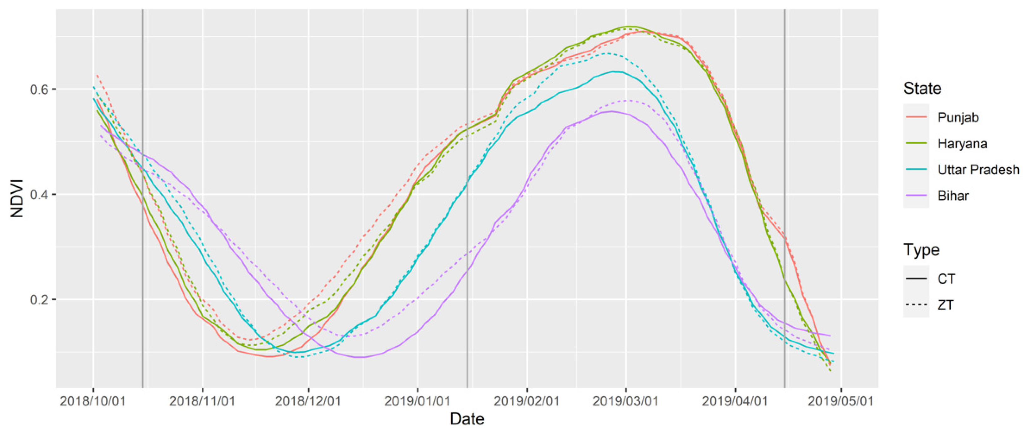
We created multi-date image composites as opposed to using single date images in our classification models. This is because there were many masked pixels due to cloud cover, and image compositing reduced the number of missing pixels across our study region. In addition, image compositing allowed us to apply our classification model across the full spatial extent of the IGP by accounting for different satellite revisit dates across the study region. We determined the image composite date range based on the phenology of wheat across our study region (Figure 2 and Figure A1A,B) and to minimize missing pixels due to cloud cover. Considering wheat phenology, we developed one image composite from October 15th to January 15th that represented the field preparation and sowing date, and a second image composite from January 15th to April 15th that represented the majority of the agricultural growing season, including the peak greenness date. The time span for each of these periods was three months to capture variation in phenology across the study region. Wheat phenologies vary across the IGP, with earlier sowing in the west and later sowing in the east (Figure 2). For each image compositing period, we extracted five percentile values to represent the range of values for each band and index—the 0th, 25th, 50th, 75th, and 100th percentile value using methods from Azzari et al. [7]. Instead of extracting one value, such as the maximum, for each band and index for each compositing period, the percentile approach allows us to better capture the range of values observed within a given compositing period. For example, 0% captures the minimum value for each band and index during the compositing period, 50% captures the midrange value, and 100% captures the maximum value. This led to 85 features selected per image compositing period across all bands and indices (Table 2). All image data were exported at a spatial resolution of 10 m from GEE and imported into R Project Software for the remainder of the analyses.

2.4. Random Forest Models and Validation

Before running the random forest model, we removed highly correlated features using a 0.9 threshold value using the ‘findCorrelation’ function in the ‘caret’ package [37] in R Project Software version 3.6.1 [28]. We removed correlated features for each individual image compositing season and both seasons combined using all pixels from all training polygons (Table 1). This reduced the number of features used in our models by approximately 50%. We conducted the random forest classification using the ‘randomForest’ package [38] in R Project Software.
Given that field sizes vary across our study region, we sampled only 10 pixels from each polygon to ensure that each polygon was weighted evenly in our model. If a field size was smaller than or equal to 10 pixels, we sampled all pixels from the polygon. We separated our field data into a training data set (70% of all polygons) and a test data set (30% of all polygons), which was used for validation. The number of ZT and CT polygons was equal in both the training and test datasets; however, the number of pixels was slightly different due to the presence of some small fields that had fewer than 10 pixels available.
We ran several random forest models to answer our four main research questions. To examine how well tillage practices can be mapped across the IGP (Research Question 1), we ran a random forest model that used all uncorrelated features from the early and main season mosaics (Figure 2). To identify whether using only early season imagery is able to accurately map tillage practices (Research Question 2), we ran an additional random forest model that used all uncorrelated features from only the early season mosaic. We ran both of these analyses only for 2018–2019, which was the year when we had large data coverage as we purposefully collected ground truth data to develop a tillage classification algorithm. For these analyses, we stratified training and validation polygons by state and tillage type.
To test whether model accuracy would change if fewer polygons were used to train our models (Research Question 3), we conducted a bootstrapping analysis [39] using four subsets of the training data—25%, 50%, 75%, and 100% of the original number of training polygons. For this analysis, we used only the early season mosaic analysis and 2018–2019 data. For validation, we used the same number of test polygons as the original model. Sampling of the subsets was done at random across all polygons and was not stratified by state or tillage type. We iterated the bootstrap analysis 400 times for each subset [40].
Finally, to examine how accurately our model performed through time (Research Question 4), we applied the random forest model that we developed using the early season mosaic in 2018–2019 to early season mosaics from 2016–2017 and 2017–2018. We then validated this model using the polygon data that we had access to from 2016–2017 (Punjab and Haryana) and 2017–2018 (Uttar Pradesh and Bihar). All models were validated at the state scale using pixels from validation polygons in each state, and at the all-IGP scale using all validation polygons across the IGP.

3. Results

3.1. Full Season Tillage Classification

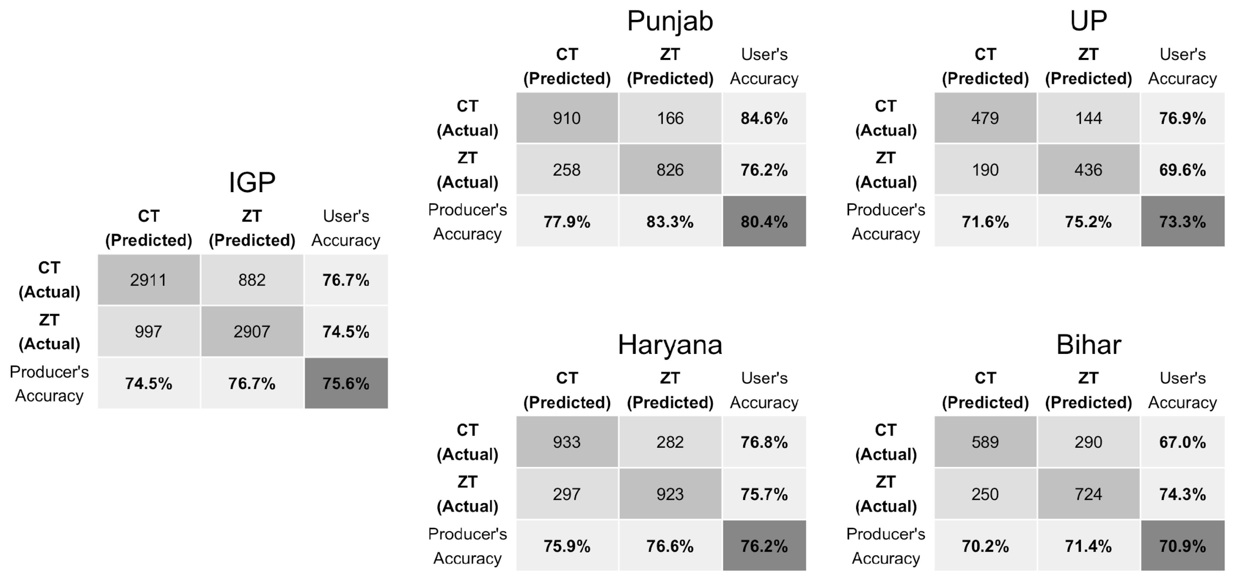
The full season classification model performed moderately well, with an overall accuracy of 75.6% across the IGP (Figure 3). Considering state-level results, there was a spatial signal in classification accuracy, with higher overall accuracies in the west (Punjab, overall accuracy of 80.4%) and lower accuracies in the east (Bihar, overall accuracy of 70.9%). Across the IGP, user’s and producer’s accuracies were similar for ZT and CT; however, this pattern was not consistent across individual states. In Punjab and Uttar Pradesh, user’s accuracy was higher for CT and producer’s accuracy was higher for ZT. In Haryana, user’s and producer’s accuracies were largely similar for CT and ZT. In Bihar, user’s accuracy was higher for ZT and producer’s accuracy was similar for ZT and CT.

3.2. Early Season Tillage Classification

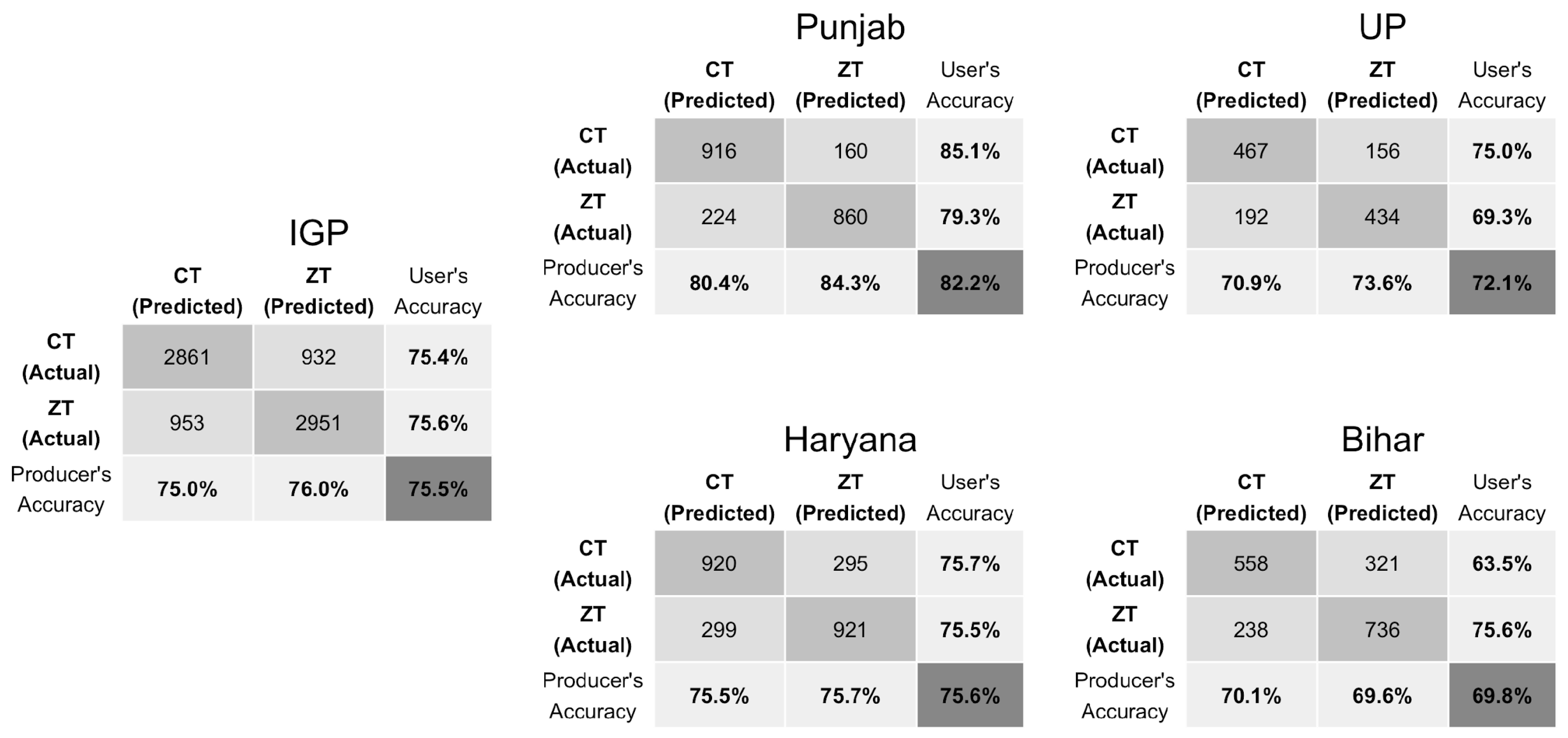
The model that used only early season mosaics performed moderately well, with an overall accuracy across the IGP of 75.5%. The results at the all-IGP and individual state scale are largely similar to the model that used mosaics from the full season. Across the IGP, user’s accuracy, producer’s accuracy, and overall accuracy for the early season model (Figure 4) were within 1% of the values from the full season model (Figure 3). Considering individual states, the same spatial pattern observed with the full season model persisted with the early season model; accuracies were highest in the west (Punjab, overall accuracy 82.2%) and lowest in the east (Bihar, overall accuracy 69.8%). Overall accuracies for individual states for the early season model (Figure 4) were within 2% of the overall accuracies reported for the full season model (Figure 3). There were larger changes in user’s and producer’s accuracies in some cases. For example, user’s accuracy and producer’s accuracy increased by up to 3% for the Punjab model, and user’s accuracy for CT decreased by approximately 4% in Bihar in the early season model (Figure 4) compared with the full season model (Figure 3).

3.3. Training Sample Size versus Model Accuracy

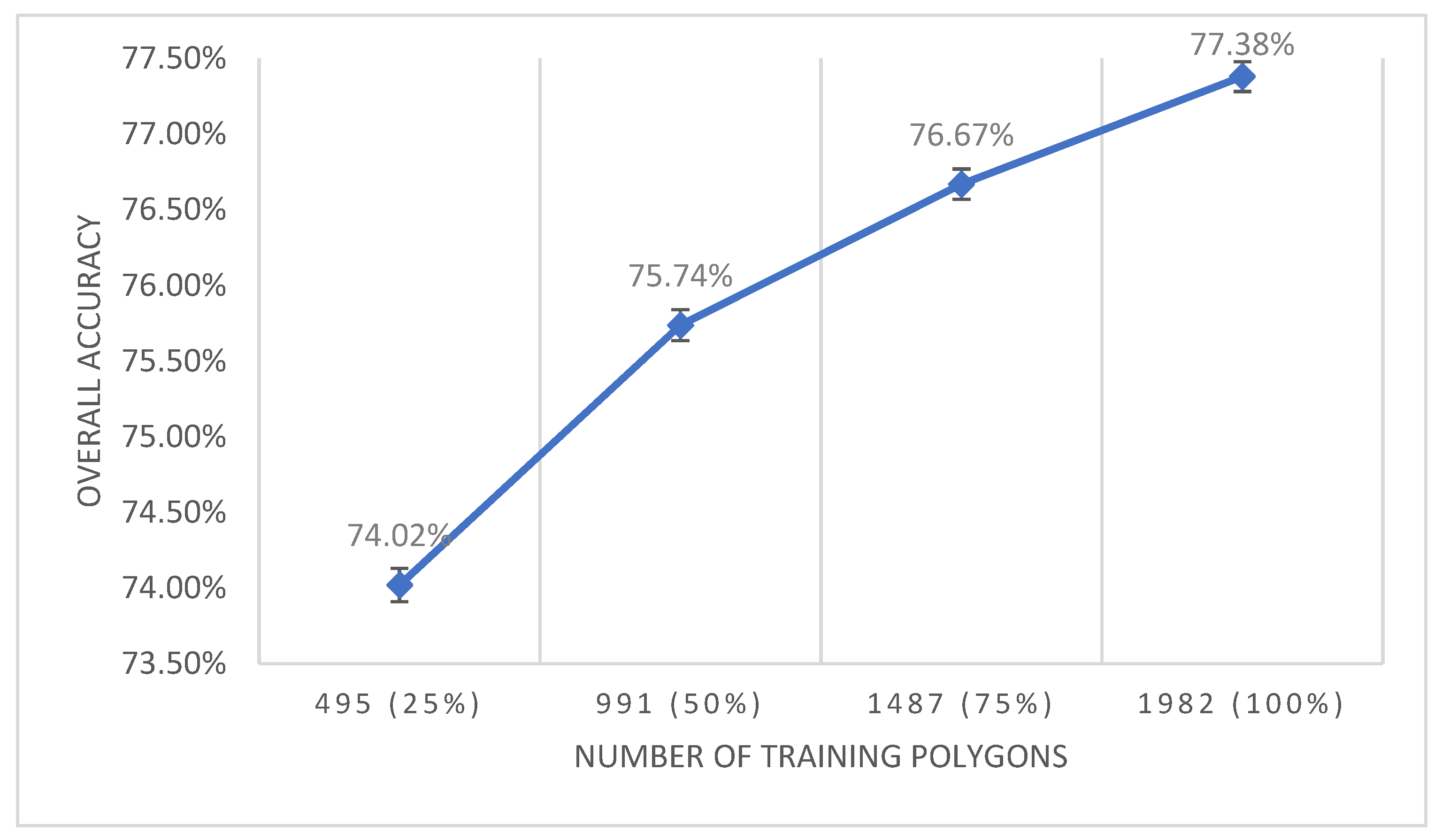
We find that our random forest classification model is sensitive to the amount of training data used, with overall accuracy significantly (p < 0.05) decreasing as the number of training polygons used decreased from 100% to 25% of all available polygons (Figure 5). The change in overall accuracy, however, was not very large and decreased by approximately 1% for every 25% reduction in the number of training samples. The difference in overall accuracy between using only 25% of all polygons, or 495 fields, was only 3% lower than using 100% of polygons, or 1982 fields, for training.

3.4. Back in Time Classification

We find that our model did not generalize well through time in the eastern IGP, in the states of Uttar Pradesh and Bihar, but did well in the western IGP, in the states of Punjab and Haryana (Figure 6). Overall accuracies decreased by approximately 10% for the overall IGP model and for the western IGP states of Punjab and Haryana compared with the 2018–2019 model. However, in the eastern IGP, overall accuracies decreased by approximately 20% in Bihar and 30% in Uttar Pradesh compared with the 2018–2019 model. Overall accuracies in Uttar Pradesh were below 50%, suggesting that the model performed worse than random assignment of fields to ZT or CT.

4. Discussion and Conclusions

To date, it has been challenging to quantify the extent of zero tillage adoption in smallholder systems, as current estimates are based on household surveys with limited spatial and temporal coverage. Remote sensing can offer a low-cost and scalable way to map tillage practices, yet to date no work has mapped zero tillage adoption in smallholder systems using satellite data. It has historically been challenging to map field-level tillage practices in smallholder systems given that the size of fields is typically smaller than the spatial resolution of readily available satellite imagery, such as Landsat (30 m) and MODIS (250 m) [12]. We show that higher spatial resolution data from Sentinel-2 can be used to map tillage practices at the field scale and at large spatio-temporal scales in smallholder systems in India. Our models have overall accuracies of approximately 75%, which are similar to the accuracies obtained in previous studies that map zero tillage practices in other parts of the world, including in the United States (e.g., [7,8]).
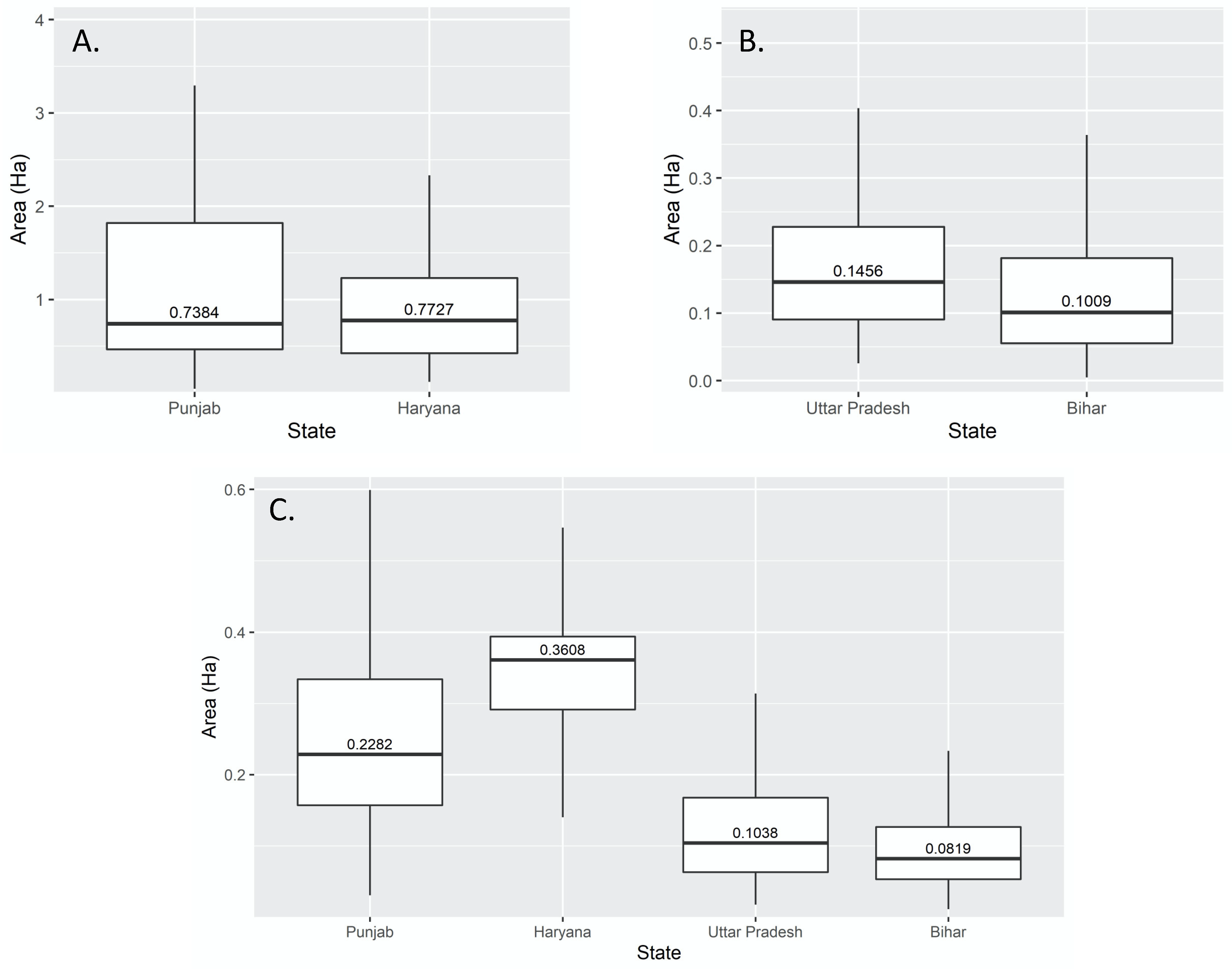
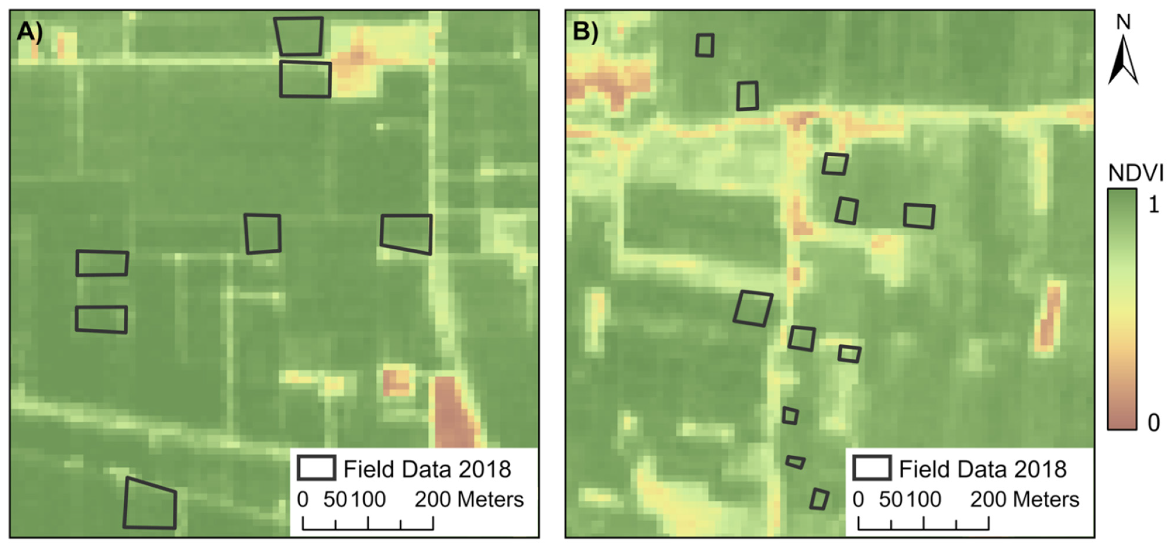
We find that overall accuracies vary across the IGP, with higher accuracies in the western IGP (Punjab and Haryana) and lower accuracies in the eastern IGP (Uttar Pradesh and Bihar). There are several reasons for why accuracies may be lower in the eastern IGP. First, fields in the western IGP are typically larger than those in the east (Figure A2). Even though we minimized the effect of field size in our analysis by including only ten pixels per polygon, 40–50% of fields in the eastern IGP were smaller than ten Sentinel-2 pixels (compared with only <6% of fields in the western IGP), and there is a higher chance of including mixed pixels at field edges in smaller fields [19] (Figure A3). Second, rice residues in ZT fields are managed differently across the IGP, as rice residues are largely cleared in the eastern IGP but retained as stubble and residue on the soil’s surface in the western IGP. It is likely more difficult to detect ZT fields when rice residues are removed as they look more similar to CT fields where residues are cleared and tilled into the soil. Third, field management is much more heterogeneous in the eastern IGP than in the west, and this likely makes it more difficult to use one algorithm to accurately map tillage practices across fields in the east. Specifically, there is large heterogeneity in planting time in the eastern IGP, where sowing dates can range from early November until early January, compared with the west, where sowing dates are largely concentrated from the end of October to the end of November [18].
Considering image timing, we find that models that used only early season mosaics led to very similar accuracies as models that used full season mosaics, which provides two important benefits. First, using only early season mosaics allows for the creation of within-season tillage maps by January of the year of interest. Second, using only early season mosaics significantly reduces computation time by reducing the amount of imagery that needs to be processed by half. This is particularly important when using Sentinel-2 Level 1-C data given that all images were exported from GEE and corrected to surface reflectance on local machines using Python. While previous studies have shown that using multi-temporal imagery throughout the growing season increases classification accuracy [8,19], our work suggests that using only multi-temporal imagery during the early part of the growing season is sufficient for mapping tillage practices in our study region.
Given the difficulty of obtaining ground data to train and validate our classification algorithm, we examined the tradeoffs between training data sample size and overall classification accuracy. We find that while overall accuracy significantly decreased as we used fewer training samples, the change in accuracy was not very large, with only a 3% drop in overall accuracy when using only 25% of all training samples (Figure 5, 495 polygons versus 1982 polygons). This suggests that it may be possible to map tillage practices using relatively small amounts of ground data.
Finally, considering the ability of our model to generalize across time, we find that overall model accuracy decreased when applied to previous years, though the decline in accuracy was not consistent across the IGP. In the western IGP, model accuracy only decreased by 5–10%, whereas in the eastern IGP, model accuracy decreased by 20–30%. These results suggest that our model can likely be applied through time in the western IGP, but not in the eastern IGP. There are several reasons our model may perform better through time in the west compared with the east. First, there is more variability in sowing patterns through time in the east; previous studies have shown that wheat planting date in the eastern IGP is sensitive to the timing of monsoon onset, and thus may fluctuate from year to year [24]. Second, it is possible that our accuracies are lower in the eastern IGP partly due to lower data quality. The field data that we used to validate our back in time model in the east were collected by farmers using mobile phones, whereas in the west, field data were collected by CIMMYT staff using GNSS units. Previous work has shown that self-report information can be inaccurate and can lead to reduced classification accuracies of remote sensing algorithms [41]. Mobile phones can also be less precise in measuring location compared with handheld GNSS units [42], which could have led to increased error when digitizing field polygon boundaries in the east. Future work should examine how well models perform through time when high-quality field data are collected over multiple years.
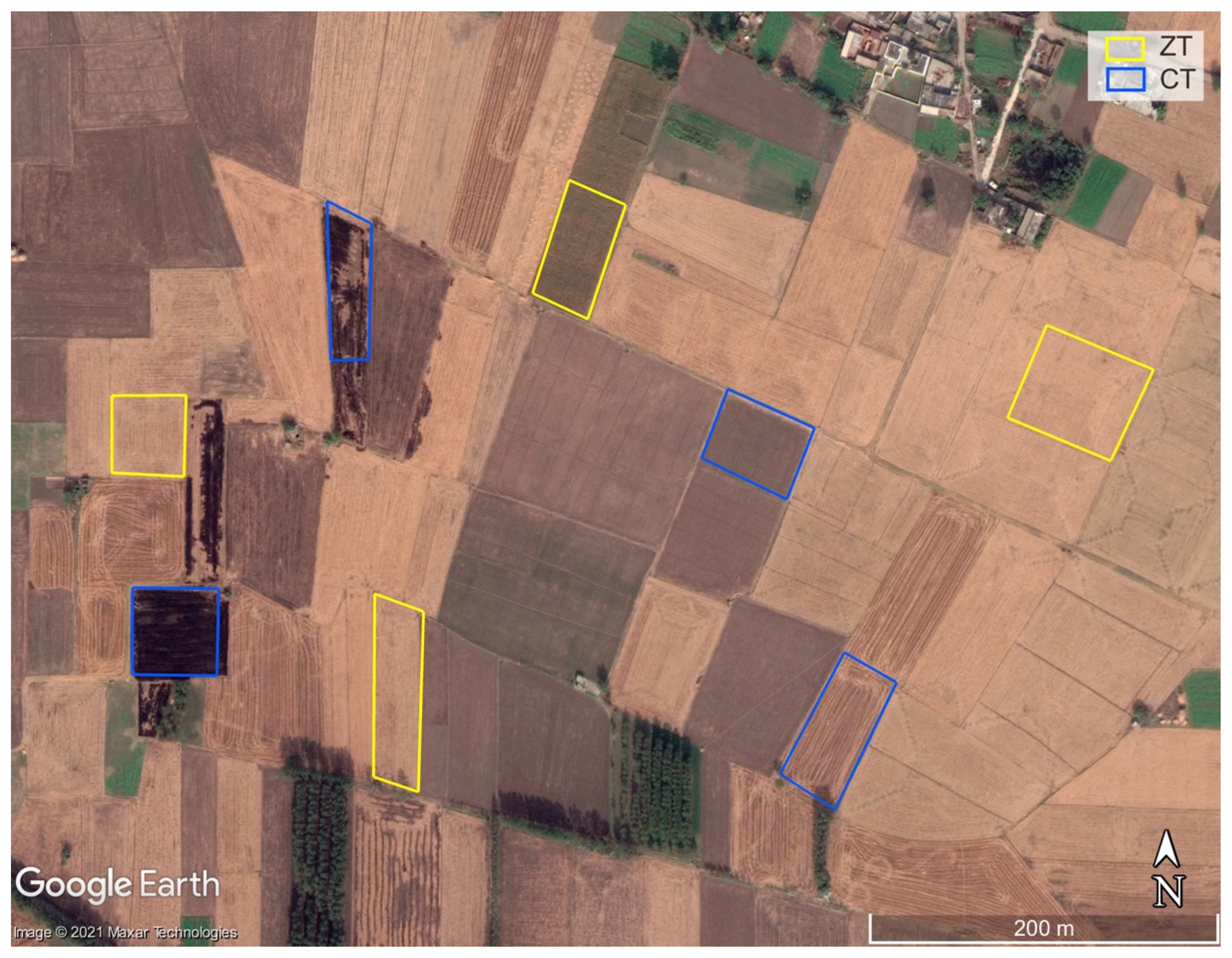
While our model achieved accuracies that are similar to other tillage mapping studies, it is possible that accuracies could be further improved by combining information from multiple sensors, such as optical and radar data, or by using higher spatial resolution imagery, such as Planet (3 m). Radar data may help improve model accuracy as it can better capture textural differences that may exist between completely cleared and tilled CT fields and ZT fields that contain crop residue (Figure A4). Higher spatial resolution data may also improve accuracies as field sizes in our study region are small, particularly in the eastern IGP, and finer spatial resolution data may reduce the occurrence of mixed pixels that occur at field edges [19]. Future work should assess the ability of these other sensors and sensor combinations to map tillage practices of smallholder farms.
In conclusion, we show that high-resolution Sentinel-2 data can be used to accurately map tillage practices at the field-scale in smallholder systems in India. We find that overall classification accuracies are moderate (~75%) and are similar to accuracies from previous studies that have mapped tillage practices in other parts of the world. We find that our model performs best in the western IGP, where field sizes are larger, crop management is more homogeneous, and zero tillage fields have higher residue retention compared with fields in the east. Our model is also able to accurately map tillage practices through time in the western IGP, with a reduction in accuracy of only 5–10% when applied to historical data. Our results highlight the ability of satellite data to map smallholder tillage practices at scale, providing a low-cost and scalable way to measure zero tillage adoption in smallholder systems.

Author Contributions

Conceptualization, M.J., M.L.J., B.S., R.S. and P.R.; data collection, S.P., D.B., L.K.S., M.K. and U.S.; methodology, M.J., W.Z., P.R. and U.S.; formal analysis, W.Z.; writing—original draft preparation, W.Z. and M.J.; writing—review and editing, all authors. All authors have read and agreed to the published version of the manuscript.

Funding

This research was funded by the NASA Land Cover and Land Use Change (LCLUC) program, grant number NNX17AH97G; the NASA New Investigator Program (NIP), grant number NNX16AI19G; Indian Council of Agricultural Research (ICAR)-W3 funds for Conservation Agriculture research; CGIAR Research Program on Wheat Agri-Food System (WHEAT) and the Standing Panel on Impact Assessment (SPIA) under the grant ‘Strengthening Impact Assessment in the CGIAR (SIAC)’.

Data Availability Statement

The codes and data used in this paper are available at https://www.dropbox.com/sh/1ltp7y1hnif8wzt/AAC92ozG54bB6El4V-jgPix0a?dl=0 (accessed on 1 November 2021). All other data are available by writing to the corresponding author M.J.

Acknowledgments

We thank the field staff of CIMMYT’s projects (CSISA, CCAFS, Wheat Agri-Food Systems) and collaborating partners (Indian Council of Agricultural Research) for supporting and collecting field data across the IGP.

Conflicts of Interest

The authors declare no conflict of interest.

Appendix A

Figure A1. Mean NDTI (A) and STI (B) phenology curves of wheat in the 2018–2019 winter growing season for each state and each tillage type.
Remotesensing 13 05108 g0a1
Figure A2. Boxplots of field size (in ha) for all 2016–2017 (A), 2017–2018 (B), and 2018–2019 (C) polygons considered in our study plotted by state. Median field size (ha) is listed for each state above the bolded line within each boxplot. Field sizes in 2016–2017 are much larger because in this year several fields were measured as all plots that farmers managed (>10 ha) and were not subdivided by individual field as was done in 2017–2018 and 2018–2019.
Remotesensing 13 05108 g0a2
Figure A3. Zoom-in of polygon overlays in Punjab (A) and Bihar (B) on Sentinel-2 Level 2A NDVI mosaics for February 2019. Field sizes are smaller in the eastern IGP (B), and this leads to increased mixed pixles at field edges compared with in the western IGP (A).
Remotesensing 13 05108 g0a3
Figure A4. Zoom-in of ZT and CT polygons from 2018–2019 in Punjab overlaid on a high-resolution image from November 2018 from Google Earth Pro. Slight visual differences are apparent between CT and ZT fields, with tillage patterns visible in most CT fields.
Remotesensing 13 05108 g0a4

References

  1. Brouder, S.M.; Gomez-Macpherson, H. The Impact of Conservation Agriculture on Smallholder Agric. Yields: A Scoping Review of the Evidence. Agric. Ecosyst. Environ. 2014, 187, 11–32. [Google Scholar] [CrossRef]
  2. El-Shater, T.; Yigezu, Y.A.; Mugera, A.; Piggin, C.; Haddad, A.; Khalil, Y.; Loss, S.; Aw-Hassan, A. Does Zero Tillage Improve the Livelihoods of Smallholder Cropping Farmers? J. Agric. Econ. 2016, 67, 154–172. [Google Scholar] [CrossRef]
  3. Erenstein, O.; Laxmi, V. Zero Tillage Impacts in India’s Rice–Wheat Systems: A Review. Soil Tillage Res. 2008, 100, 1–14. [Google Scholar] [CrossRef]
  4. Mondal, S.; Chakraborty, D.; Bandyopadhyay, K.; Aggarwal, P.; Rana, D.S. A Global Analysis of the Impact of Zero-Tillage on Soil Physical Condition, Organic Carbon Content, and Plant Root Response. Land Degrad. Dev. 2020, 31, 557–567. [Google Scholar] [CrossRef]
  5. Jat, M.L.; Chakraborty, D.; Ladha, J.K.; Rana, D.S.; Gathala, M.K.; McDonald, A.; Gerard, B. Conservation Agriculture for Sustainable Intensification in South Asia. Nat. Sustain. 2020, 3, 336–343. [Google Scholar] [CrossRef]
  6. Jain, M.; Singh, B. Toward an Evergreen Revolution sustainable intensification in smallholder farming. In A Better Planet: Forty Big Ideas for a Sustainable Future; Etsy, D., Burke, I., Eds.; Yale University Press: London, UK, 2019; ISBN 978-0-300-24889-0. [Google Scholar]
  7. Azzari, G.; Grassini, P.; Edreira, J.I.R.; Conley, S.; Mourtzinis, S.; Lobell, D.B. Satellite Mapping of Tillage Practices in the North Central US Region from 2005 to 2016. Remote Sens. Environ. 2019, 221, 417–429. [Google Scholar] [CrossRef]
  8. Zheng, B.; Campbell, J.B.; Shao, Y.; Wynne, R.H. Broad-Scale Monitoring of Tillage Practices Using Sequential Landsat Imagery. Soil Sci. Soc. Am. J. 2013, 77, 1755–1764. [Google Scholar] [CrossRef]
  9. Steckel, J.C.; Dorband, I.I.; Montrone, L.; Ward, H.; Missbach, L.; Hafner, F.; Jakob, M.; Renner, S. Distributional Impacts of Carbon Pricing in Developing Asia. Nat. Sustain. 2021, 4, 1005–1014. [Google Scholar] [CrossRef]
  10. Bricklemyer, R.S.; Lawrence, R.L.; Miller, P.R.; Battogtokh, N. Predicting Tillage Practices and Agric. Soil Disturbance in North Central Montana with Landsat Imagery. Agric. Ecosyst. Environ. 2006, 114, 210–216. [Google Scholar] [CrossRef]
  11. Sharma, S.; Dhakal, K.; Wagle, P.; Kilic, A. Retrospective Tillage Differentiation Using the Landsat-5 TM Archive with Discriminant Analysis. Agrosyst. Geosci. Environ. 2020, 3, e20000. [Google Scholar] [CrossRef] [Green Version]
  12. Jain, M.; Srivastava, A.K.; Singh, B.; McDonald, A.; Malik, R.K.; Lobell, D.B. Mapping Smallholder Wheat Yields and Sowing Dates Using Micro-Satellite Data. Remote Sens. 2016, 8, 860. [Google Scholar] [CrossRef] [Green Version]
  13. Watts, J.D.; Powell, S.L.; Lawrence, R.L.; Hilker, T. Improved Classification of Conservation Tillage Adoption Using High Temporal and Synthetic Satellite Imagery. Remote Sens. Environ. 2011, 115, 66–75. [Google Scholar] [CrossRef]
  14. Immitzer, M.; Vuolo, F.; Atzberger, C. First Experience with Sentinel-2 Data for Crop and Tree Species Classifications in Central Europe. Remote Sens. 2016, 8, 166. [Google Scholar] [CrossRef]
  15. Xie, Q.; Dash, J.; Huete, A.; Jiang, A.; Yin, G.; Ding, Y.; Peng, D.; Hall, C.C.; Brown, L.; Shi, Y.; et al. Retrieval of Crop Biophysical Parameters from Sentinel-2 Remote Sensing Imagery. Int. J. Appl. Earth Obs. Geoinf. 2019, 80, 187–195. [Google Scholar] [CrossRef]
  16. Ding, Y.; Zhang, H.; Wang, Z.; Xie, Q.; Wang, Y.; Liu, L.; Hall, C.C. A Comparison of Estimating Crop Residue Cover from Sentinel-2 Data Using Empirical Regressions and Machine Learning Methods. Remote Sens. 2020, 12, 1470. [Google Scholar] [CrossRef]
  17. Najafi, P.; Navid, H.; Feizizadeh, B.; Eskandari, I.; Blaschke, T. Fuzzy Object-Based Image Analysis Methods Using Sentinel-2A and Landsat-8 Data to Map and Characterize Soil Surface Residue. Remote Sens. 2019, 11, 2583. [Google Scholar] [CrossRef] [Green Version]
  18. Jain, M.; Singh, B.; Srivastava, A.A.K.; Malik, R.K.; McDonald, A.J.; Lobell, D.B. Using Satellite Data to Identify the Causes of and Potential Solutions for Yield Gaps in India’s Wheat Belt. Environ. Res. Lett. 2017, 12, 094011. [Google Scholar] [CrossRef]
  19. Rao, P.; Zhou, W.; Bhattarai, N.; Srivastava, A.K.; Singh, B.; Poonia, S.; Lobell, D.B.; Jain, M. Using Sentinel-1, Sentinel-2, and Planet Imagery to Map Crop Type of Smallholder Farms. Remote Sens. 2021, 13, 1870. [Google Scholar] [CrossRef]
  20. Zheng, B.; Campbell, J.B.; de Beurs, K.M. Remote Sensing of Crop Residue Cover Using Multi-Temporal Landsat Imagery. Remote Sens. Environ. 2012, 117, 177–183. [Google Scholar] [CrossRef]
  21. Collins, L.; McCarthy, G.; Mellor, A.; Newell, G.; Smith, L. Training Data Requirements for Fire Severity Mapping Using Landsat Imagery and Random Forest. Remote Sens. Environ. 2020, 245, 111839. [Google Scholar] [CrossRef]
  22. Millard, K.; Richardson, M. On the Importance of Training Data Sample Selection in Random Forest Image Classification: A Case Study in Peatland Ecosystem Mapping. Remote Sens. 2015, 7, 8489–8515. [Google Scholar] [CrossRef] [Green Version]
  23. Xu, J.; Zhu, Y.; Zhong, R.; Lin, Z.; Xu, J.; Jiang, H.; Huang, J.; Li, H.; Lin, T. DeepCropMapping: A Multi-Temporal Deep Learning Approach with Improved Spatial Generalizability for Dynamic Corn and Soybean Mapping. Remote Sens. Environ. 2020, 247, 111946. [Google Scholar] [CrossRef]
  24. Newport, D.; Lobell, D.B.; Balwinder-Singh; Srivastava, A.K.; Rao, P.; Umashaanker, M.; Malik, R.K.; McDonald, A.; Jain, M. Factors Constraining Timely Sowing of Wheat as an Adaptation to Climate Change in Eastern India. Weather Clim. Soc. 2020, 12, 515–528. [Google Scholar] [CrossRef]
  25. Tittonell, P.; Vanlauwe, B.; Leffelaar, P.A.; Rowe, E.C.; Giller, K.E. Exploring Diversity in Soil Fertility Management of Smallholder Farms in Western Kenya: I. Heterogeneity at Region and Farm Scale. Agric. Ecosyst. Environ. 2005, 110, 149–165. [Google Scholar] [CrossRef]
  26. Jain, M.; Mondal, P.; Galford, G.; Fiske, G.; DeFries, R. An Automated Approach to Map Winter Cropped Area of Smallholder Farms across Large Scales Using MODIS Imagery. Remote Sens. 2017, 9, 566. [Google Scholar] [CrossRef] [Green Version]
  27. Keil, A.; D’Souza, A.; McDonald, A. Growing the Service Economy for Sustainable Wheat Intensification in the Eastern Indo-Gangetic Plains: Lessons from Custom Hiring Services for Zero-Tillage. Food Secur. 2016, 18, 1011–1028. [Google Scholar] [CrossRef] [Green Version]
  28. R Core Team. R: A Language and Environment for Statistical Computing; R Foundation for Statistical Computing: Vienna, Austria, 2021; Available online: https://www.R-project.org/ (accessed on 1 November 2021).
  29. Gorelick, N.; Hancher, M.; Dixon, M.; Ilyushchenko, S.; Thau, D.; Moore, R. Google Earth Engine: Planetary-Scale Geospatial Analysis for Everyone. Remote Sens. Environ. 2017, 202, 18–27. [Google Scholar] [CrossRef]
  30. Murphy, S. Atmospherically Corrected Time Series Using Google Earth Engine. 2018. Available online: https://github.com/samsammurphy/ee-atmcorr-timeseries (accessed on 1 November 2021).
  31. Wilson, R.T. Py6S: A Python Interface to the 6S Radiative Transfer Model. Comput. Geosci. 2013, 51, 166–171. [Google Scholar] [CrossRef] [Green Version]
  32. Remote Estimation of Leaf Area Index and Green Leaf Biomass in Maize Canopies-Gitelson-2003-Geophysical Research Letters-Wiley Online Library. Available online: https://agupubs-onlinelibrary-wiley-com.proxy.lib.umich.edu/doi/full/10.1029/2002GL016450 (accessed on 4 March 2021).
  33. Carlson, T.N.; Ripley, D.A. On the Relation between NDVI, Fractional Vegetation Cover, and Leaf Area Index. Remote Sens. Environ. 1997, 62, 241–252. [Google Scholar] [CrossRef]
  34. van Deventer, A.P.; Ward, A.D.; Gowda, P.H.; Lyon, J.G. Using Thematic Mapper Data to Identify Contrasting Soil Plains and Tillage Practices. Photogramm. Eng. Remote Sens. 1997, 63, 87–93. [Google Scholar]
  35. McNairn, H.; Protz, R. Mapping Corn Residue Cover on Agricultural Fields in Oxford County, Ontario, Using Thematic Mapper. Can. J. Remote Sens. 1993, 19, 152–159. [Google Scholar] [CrossRef]
  36. Sullivan, D.G.; Truman, C.C.; Schomberg, H.H.; Endale, D.M.; Strickland, T.C. Evaluating Techniques for Determining Tillage Regime in the Southeastern Coastal Plain and Piedmont. Agron. J. 2006, 98, 1236–1246. [Google Scholar] [CrossRef]
  37. Kuhn, M. Caret: Classification and Regression Training. R Package Version 6.0-88. 2021. Available online: https://CRAN.R-project.org/package=caret (accessed on 1 November 2021).
  38. Liawm, A.; Wiener, M. Classification and Regression by randomForest. R News 2002, 2, 18–22. [Google Scholar]
  39. Efron, B.; Tibshirani, R.J. An Introduction to the Bootstrap, 1st ed.; Chapman and Hall/CRC: New York, NY, USA, 1994. [Google Scholar]
  40. Davidson, R.; MacKinnon, J.G. Bootstrap Tests: How Many Bootstraps? Econom. Rev. 2000, 19, 55–68. [Google Scholar] [CrossRef] [Green Version]
  41. Paliwal, A.; Jain, M. The Accuracy of Self-Reported Crop Yield Estimates and Their Ability to Train Remote Sensing Algorithms. Front. Sustain. Food Syst. 2020, 4, 25. [Google Scholar] [CrossRef] [Green Version]
  42. Merry, K.; Bettinger, P. Smartphone GPS Accuracy Study in an Urban Environment. PLoS ONE 2019, 14, e0219890. [Google Scholar] [CrossRef] [Green Version]
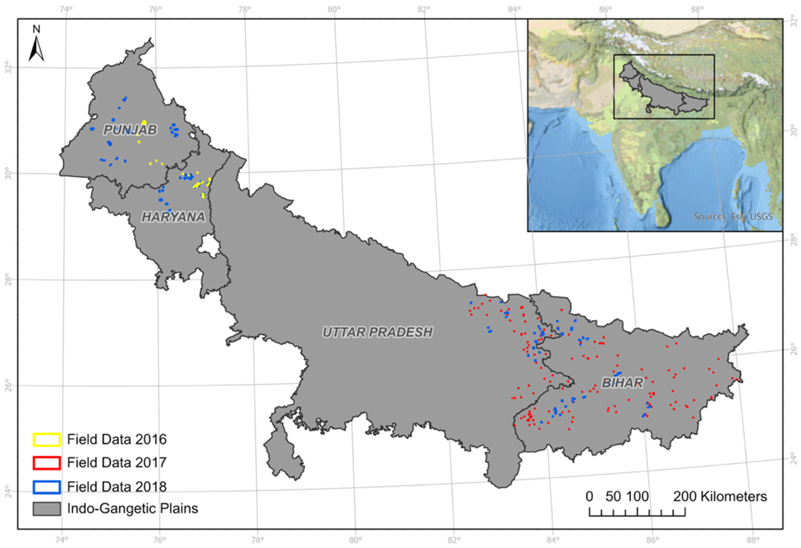
Figure 1. Map of the study area (highlighted in gray) and field data (highlighted in yellow, red, and blue).
Remotesensing 13 05108 g001
Figure 2. Mean NDVI phenology curve of wheat in the 2018–2019 winter growing season for each state and each tillage type.
Remotesensing 13 05108 g002
Figure 3. Confusion matrices for all-IGP and individual state validation for the model that uses full season mosaics. Overall accuracy is highlighted in the dark gray squares in each table.
Remotesensing 13 05108 g003
Figure 4. Confusion matrices for all-IGP and individual state validation for the model that uses only the early season mosaic. Overall accuracy is highlighted in the dark gray squares in each table.
Remotesensing 13 05108 g004
Figure 5. Mean overall accuracies and 95% confidence intervals of early season random forest classification models when using different numbers of training data (25% to 100% of the training polygons available) in a bootstrap analysis (n = 400).
Remotesensing 13 05108 g005
Figure 6. Confusion matrices for all-IGP and individual state validation for the model that uses only the early season mosaics from 2018 to 2019 and applies them back in time. Overall accuracy is highlighted in the dark gray squares in each table.
Remotesensing 13 05108 g006
Table 1. Total number of field polygons used from each year and each state for training and testing.
StateTotal Polygons 2018–2019Total Polygons 2017–2018Total Polygons 2016–2017
Punjab7360238
Haryana8140134
Uttar Pradesh502720
Bihar7781200
Table 2. Bands and indices used in the random forest classification.
BandsDescriptionIndexFormula
B2BlueGCVI(NIR/Green)
B3GreenNDVI(NIR − Red)/(NIR + Red)
B4RedNDTI(SWIR1 − SWIR2)/(SWIR1 + SWIR2)
B5Red Edge 1NDI5(NIR − SWIR1)/(NIR + SWIR1)
B6Red Edge 2NDI7(NIR − SWIR2)/(NIR + SWIR2)
B7Red Edge 3CRC(SWIR1 − Green)/(SWIR1 + Green)
B8Near-Infrared (NIR)STISWIR1/SWIR2
B8ARed Edge 4
B11Short-Wave Infrared 1 (SWIR1)
B12Short-Wave Infrared 1 (SWIR1)
Publisher’s Note: MDPI stays neutral with regard to jurisdictional claims in published maps and institutional affiliations.