
Optical and Thermal Remote Sensing for Monitoring Agricultural Drought

 , ,
, ,  , ,
, ,  ,
,  ,
,  , and
, and
Abstract
:
1. Introduction
- 1
- Optical and thermal data are the most widely used in identifying vegetation conditions, soil water status, and evapotranspiration [17];
- 2
- Microwave remote sensing has a direct and solid link to soil moisture, which is a crucial indicator of agricultural drought [18];
- 3
- LiDAR is the best approach to obtaining structural information of vegetation, and it can also be used to retrieve various biochemical variables such as leaf water content [19];
- 4
- Gravity measurement is essential for monitoring groundwater; thus, it can be utilized to monitor those regions where groundwater is massively used for irrigation, especially when drought occurs [20].
2. Optical Remote Sensing
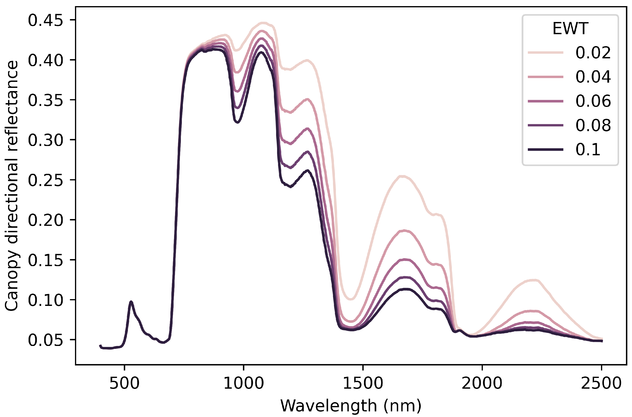
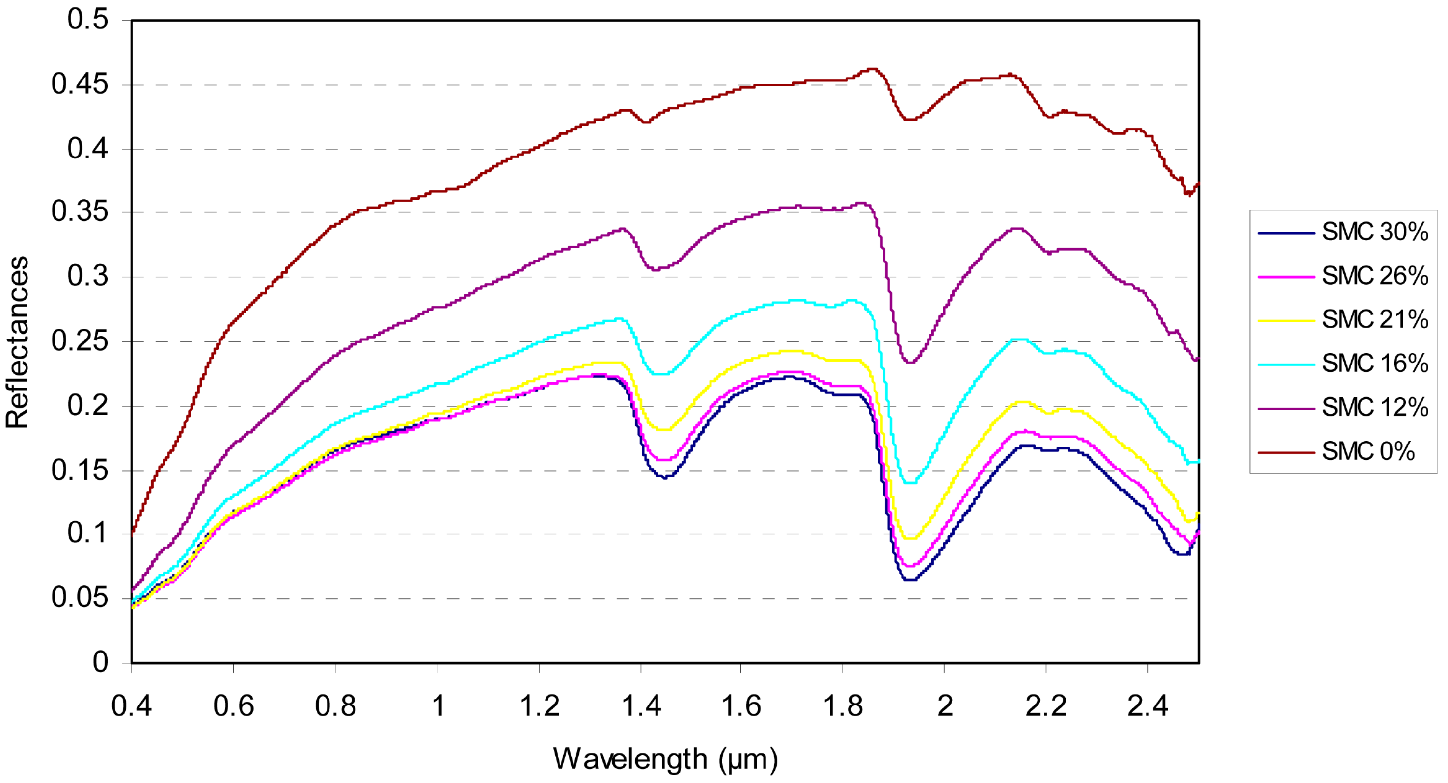
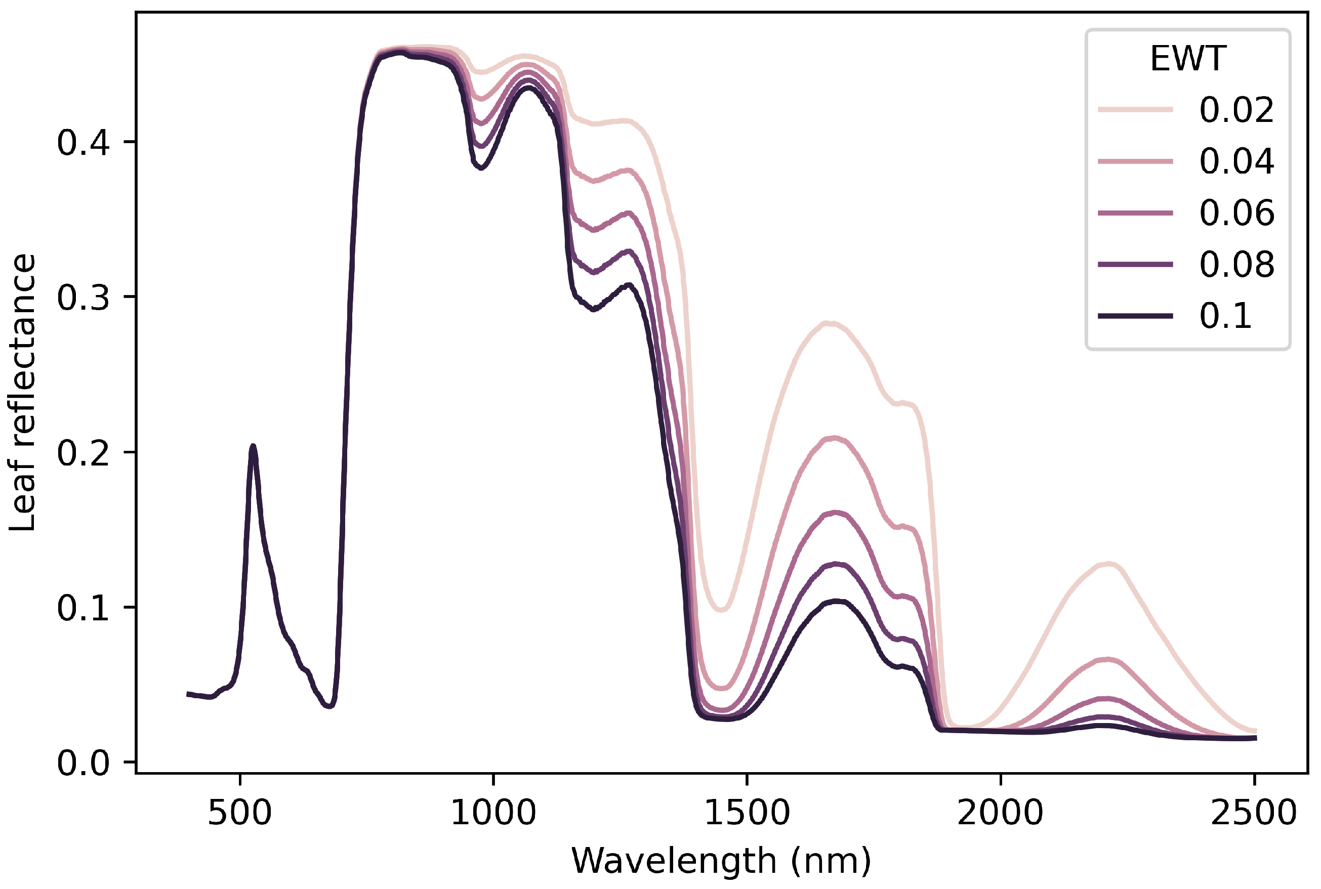
2.1. The Effect of Water Content on Soil and Crop Reflectance in the Solar Region (400–2500 nm)
2.2. Spectral Indices as Drought Indicators
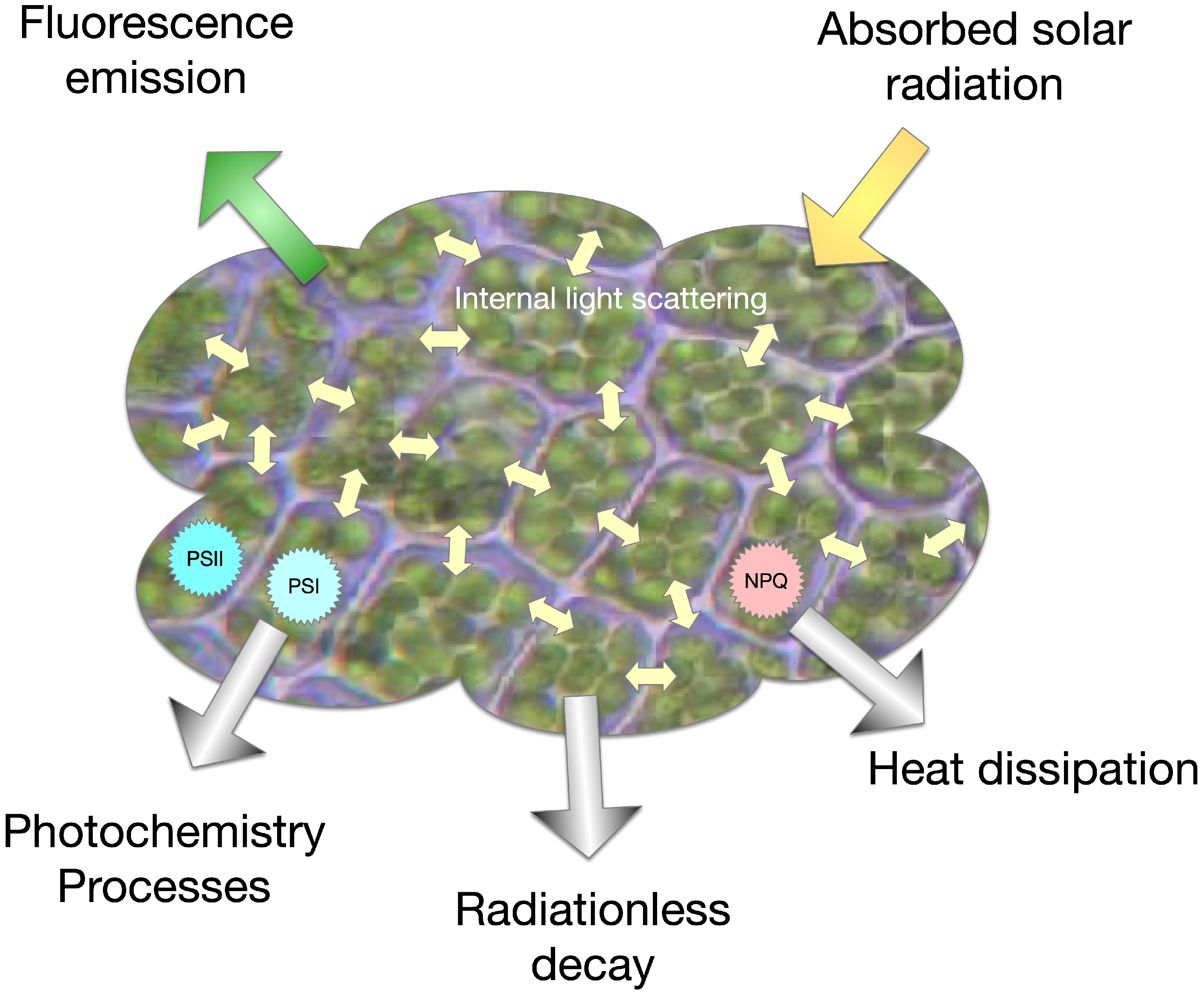
2.3. Solar-Induced Chlorophyll Fluorescence as an Early Drought Indicator
3. Thermal Remote Sensing
3.1. Thermal Properties of Crops and Soil
3.2. Thermal Inertia as a Drought Indicator
3.3. Temperature-Based Drought Indices
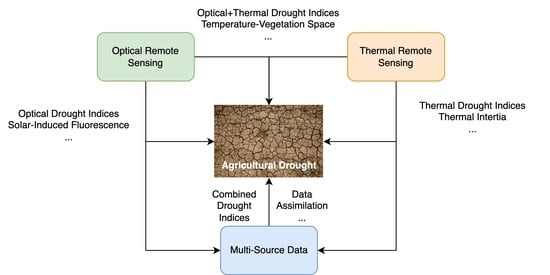
4. Combination of Optical and Thermal Remote Sensing
4.1. Simple Integrations
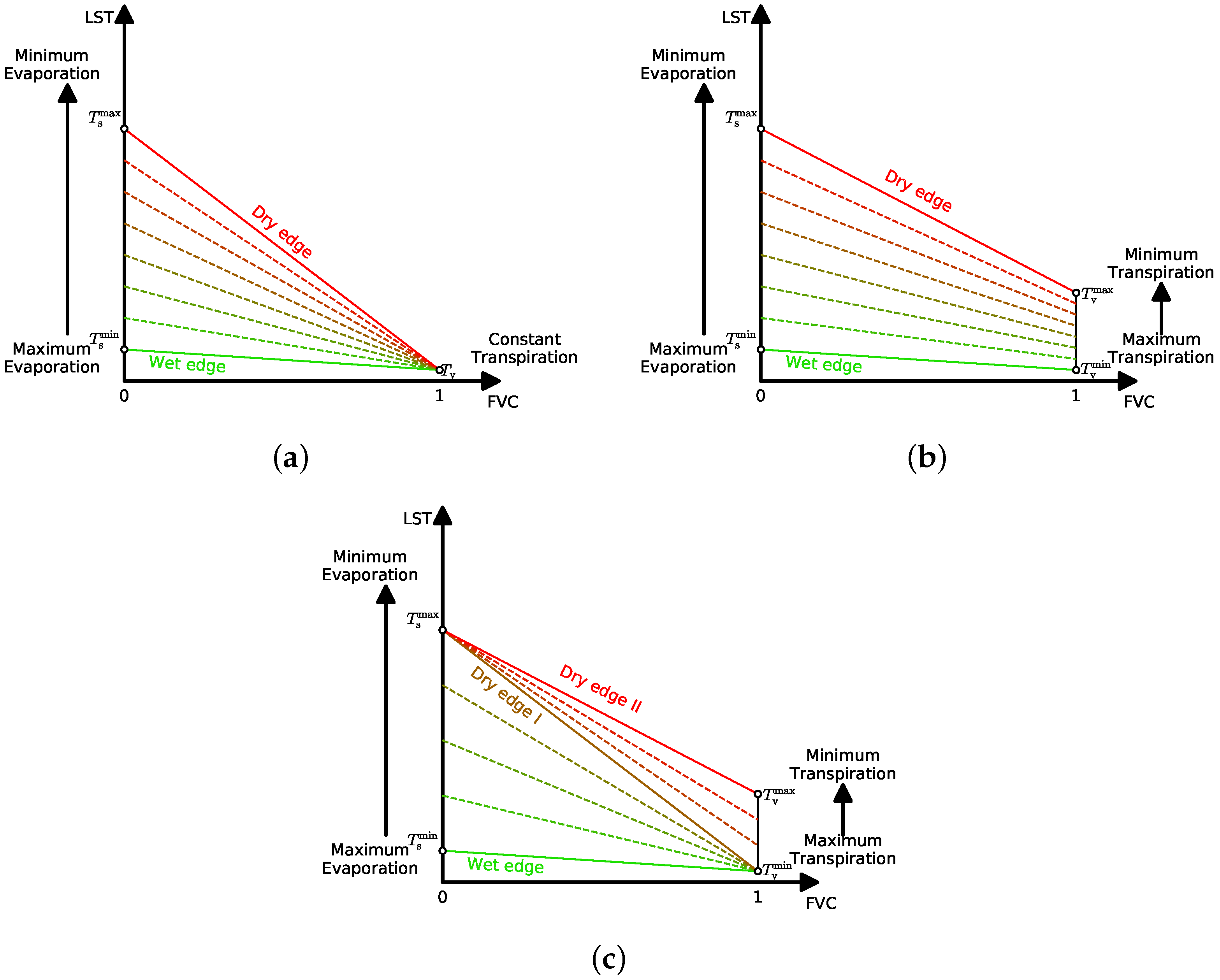
4.2. The Concept of Temperature-Vegetation Space
4.3. Applications of the Temperature-Vegetation Space in Drought Monitoring
5. Multi-Source Data and Data Assimilation
5.1. Combination of Remote Sensing and Other Data Sources
5.2. Data Assimilation
6. Perspectives
6.1. Early Detection of Drought
6.2. Improvements in Spatiotemporal Resolution
6.3. Organic Combination with Other Data Sources
6.4. Smart Prediction and Assessment
Author Contributions
Funding
Institutional Review Board Statement
Informed Consent Statement
Data Availability Statement
Conflicts of Interest
References
- Wilhite, D.A. Droughts: A Global Assesment; Routledge: Oxfordshire, UK, 2016; pp. 3–18. [Google Scholar]
- Montz, B.E.; Tobin, G.A.; Hagelman, R.R. Natural Hazards: Explanation and Integration; Guilford Publications: New York, NY, USA, 2017. [Google Scholar]
- Tannehill, I.R. Drought, Its Causes and Effects; LWW: Philadelphia, PA, USA, 1947. [Google Scholar]
- Wilhite, D.A.; Glantz, M.H. Understanding: The Drought Phenomenon: The Role of Definitions. Water Int. 1985, 10, 111–120. [Google Scholar] [CrossRef] [Green Version]
- American Meteorological Society. Policy Statement: Meteorological Drought. Bull. Am. Meteorol. Soc. 1997, 78, 847–849. [Google Scholar] [CrossRef] [Green Version]
- Mishra, A.K.; Singh, V.P. A Review of Drought Concepts. J. Hydrol. 2010, 391, 202–216. [Google Scholar] [CrossRef]
- Van Loon, A.F.; Gleeson, T.; Clark, J.; Van Dijk, A.I.; Stahl, K.; Hannaford, J.; Di Baldassarre, G.; Teuling, A.J.; Tallaksen, L.M.; Uijlenhoet, R.; et al. Drought in the Anthropocene. Nat. Geosci. 2016, 9, 89. [Google Scholar] [CrossRef] [Green Version]
- Van Loon, A.F.; Stahl, K.; Di Baldassarre, G.; Clark, J.; Rangecroft, S.; Wanders, N.; Gleeson, T.; Van Dijk, A.I.J.M.; Tallaksen, L.M.; Hannaford, J.; et al. Drought in a Human-Modified World: Reframing Drought Definitions, Understanding, and Analysis Approaches. Hydrol. Earth Syst. Sci. 2016, 20, 3631–3650. [Google Scholar] [CrossRef] [Green Version]
- Dai, A. Drought under Global Warming: A Review: Drought under Global Warming. Wiley Interdiscip. Rev. Clim. Chang. 2011, 2, 45–65. [Google Scholar] [CrossRef] [Green Version]
- Dai, A. Increasing Drought under Global Warming in Observations and Models. Nat. Clim. Chang. 2013, 3, 52–58. [Google Scholar] [CrossRef]
- Hanson, R.L. Evapotranspiration and droughts. In National Water Summary 1988–89: Hydrologic Events and Floods and Droughts (US Geological Survey Water-Supply Paper 2375); US Government Printing Office: Washington, DC, USA, 1991; pp. 99–104. [Google Scholar]
- Jaleel, C.A.; Manivannan, P.; Wahid, A.; Farooq, M.; Al-Juburi, H.J.; Somasundaram, R.; Panneerselvam, R. Drought Stress in Plants: A Review on Morphological Characteristics and Pigments Composition. Int. J. Agric. Biol. 2009, 11, 100–105. [Google Scholar]
- Li, Y.; Ye, W.; Wang, M.; Yan, X. Climate Change and Drought: A Risk Assessment of Crop-Yield Impacts. Clim. Res. 2009, 39, 31–46. [Google Scholar] [CrossRef]
- Kincer, J.B. The Seasonal Distribution of Precipitation and Its Frequency and Intensity in the United States. Mon. Weather Rev. 1919, 47, 624–631. [Google Scholar] [CrossRef]
- Sabaghy, S.; Walker, J.P.; Renzullo, L.J.; Jackson, T.J. Spatially Enhanced Passive Microwave Derived Soil Moisture: Capabilities and Opportunities. Remote Sens. Environ. 2018, 209, 551–580. [Google Scholar] [CrossRef]
- Rhee, J.; Im, J.; Carbone, G.J. Monitoring Agricultural Drought for Arid and Humid Regions Using Multi-Sensor Remote Sensing Data. Remote Sens. Environ. 2010, 114, 2875–2887. [Google Scholar] [CrossRef]
- AghaKouchak, A.; Farahmand, A.; Melton, F.S.; Teixeira, J.; Anderson, M.C.; Wardlow, B.D.; Hain, C.R. Remote Sensing of Drought: Progress, Challenges and Opportunities: Remote Sensing of Drought. Rev. Geophys. 2015, 53, 452–480. [Google Scholar] [CrossRef] [Green Version]
- Njoku, E.G.; Entekhabi, D. Passive Microwave Remote Sensing of Soil Moisture. J. Hydrol. 1996, 184, 101–129. [Google Scholar] [CrossRef]
- Zhu, X.; Wang, T.; Skidmore, A.K.; Darvishzadeh, R.; Niemann, K.; Liu, J. Canopy Leaf Water Content Estimated Using Terrestrial LiDAR. Agric. For. Meteorol. 2017, 232, 152–162. [Google Scholar] [CrossRef]
- Frappart, F.; Ramillien, G. Monitoring Groundwater Storage Changes Using the Gravity Recovery and Climate Experiment (GRACE) Satellite Mission: A Review. Remote Sens. 2018, 10, 829. [Google Scholar] [CrossRef] [Green Version]
- Engman, E.T. Progress in Microwave Remote Sensing of Soil Moisture. Can. J. Remote Sens. 1990, 16, 6–14. [Google Scholar] [CrossRef]
- Kornelsen, K.C.; Coulibaly, P. Advances in Soil Moisture Retrieval from Synthetic Aperture Radar and Hydrological Applications. J. Hydrol. 2013, 476, 460–489. [Google Scholar] [CrossRef]
- Lv, S.; Zeng, Y.; Wen, J.; Zhao, H.; Su, Z. Estimation of Penetration Depth from Soil Effective Temperature in Microwave Radiometry. Remote Sens. 2018, 10, 519. [Google Scholar] [CrossRef] [Green Version]
- Calvet, J.C.; Wigneron, J.P.; Walker, J.; Karbou, F.; Chanzy, A.; Albergel, C. Sensitivity of Passive Microwave Observations to Soil Moisture and Vegetation Water Content: L-Band to W-Band. IEEE Trans. Geosci. Remote Sens. 2011, 49, 1190–1199. [Google Scholar] [CrossRef]
- Liu, Y.; Dorigo, W.; Parinussa, R.; de Jeu, R.; Wagner, W.; McCabe, M.; Evans, J.; van Dijk, A. Trend-Preserving Blending of Passive and Active Microwave Soil Moisture Retrievals. Remote Sens. Environ. 2012, 123, 280–297. [Google Scholar] [CrossRef]
- Du, J.; Kimball, J.S.; Jones, L.A. Passive Microwave Remote Sensing of Soil Moisture Based on Dynamic Vegetation Scattering Properties for AMSR-E. IEEE Trans. Geosci. Remote Sens. 2015, 54, 597–608. [Google Scholar] [CrossRef]
- Ebtehaj, A.; Bras, R.L. A Physically Constrained Inversion for High-Resolution Passive Microwave Retrieval of Soil Moisture and Vegetation Water Content in L-Band. Remote Sens. Environ. 2019, 233, 111346. [Google Scholar] [CrossRef]
- Karthikeyan, L.; Pan, M.; Wanders, N.; Kumar, D.N.; Wood, E.F. Four Decades of Microwave Satellite Soil Moisture Observations: Part 1. A Review of Retrieval Algorithms. Adv. Water Resour. 2017, 109, 106–120. [Google Scholar] [CrossRef]
- Karthikeyan, L.; Pan, M.; Wanders, N.; Kumar, D.N.; Wood, E.F. Four Decades of Microwave Satellite Soil Moisture Observations: Part 2. Product Validation and Inter-Satellite Comparisons. Adv. Water Resour. 2017, 109, 236–252. [Google Scholar] [CrossRef]
- Heim, R.R., Jr. A Review of Twentieth-Century Drought Indices Used in the United States. Bull. Am. Meteorol. Soc. 2002, 83, 1149–1166. [Google Scholar] [CrossRef] [Green Version]
- Zargar, A.; Sadiq, R.; Naser, B.; Khan, F.I. A Review of Drought Indices. Environ. Rev. 2011, 19, 333–349. [Google Scholar] [CrossRef]
- Eisenberg, D.; Kauzmann, W.; Kauzmann, W. The Structure and Properties of Water; Oxford University Press on Demand: Oxford, UK, 2005. [Google Scholar]
- Wozniak, B.; Dera, J. Light Absorption in Sea Water; Springer: Berlin/Heidelberg, Germany, 2007; Volume 33. [Google Scholar]
- Bablet, A.; Vu, P.V.H.; Jacquemoud, S.; Viallefont-Robinet, F.; Fabre, S.; Briottet, X.; Sadeghi, M.; Whiting, M.L.; Baret, F.; Tian, J. MARMIT: A Multilayer Radiative Transfer Model of Soil Reflectance to Estimate Surface Soil Moisture Content in the Solar Domain (400–2500 Nm). Remote Sens. Environ. 2018, 217, 1–17. [Google Scholar] [CrossRef] [Green Version]
- Angström, A. The Albedo of Various Surfaces of Ground. Geogr. Ann. 1925, 7, 323–342. [Google Scholar]
- Patel, A.N. Studies on Variation of Spectral Signatures in Relation to Certain Geotechnical Properties of Soil Samples. Ph.D. Thesis, University of Indore, Indore, India, 1979. [Google Scholar]
- Neema, D.L.; Shah, A.; Patel, A.N. A Statistical Optical Model for Light Reflection and Penetration through Sand. Int. J. Remote Sens. 1987, 8, 1209–1217. [Google Scholar] [CrossRef]
- Liu, W.; Baret, F.; Gu, X.; Tong, Q.; Zheng, L.; Zhang, B. Relating Soil Surface Moisture to Reflectance. Remote Sens. Environ. 2002, 81, 238–246. [Google Scholar] [CrossRef]
- Lobell, D.B.; Asner, G.P. Moisture Effects on Soil Reflectance. Soil Sci. Soc. Am. J. 2002, 66, 6. [Google Scholar] [CrossRef]
- Mouazen, A.M.; Karoui, R.; De Baerdemaeker, J.; Ramon, H. Characterization of Soil Water Content Using Measured Visible and near Infrared Spectra. Soil Sci. Soc. Am. J. 2006, 70, 1295–1302. [Google Scholar] [CrossRef]
- Peng, J.; Shen, H.; Wu, J.S. Soil Moisture Retrieving Using Hyperspectral Data with the Application of Wavelet Analysis. Environ. Earth Sci. 2013, 69, 279–288. [Google Scholar] [CrossRef]
- Fabre, S.; Briottet, X.; Lesaignoux, A. Estimation of Soil Moisture Content from the Spectral Reflectance of Bare Soils in the 0.4–2.5 Mm Domain. Sensors 2015, 15, 3262–3281. [Google Scholar] [CrossRef]
- Curran, P.J. Remote Sensing of Foliar Chemistry. Remote Sens. Environ. 1989, 30, 271–278. [Google Scholar] [CrossRef]
- Thomas, J.R.; Namken, L.N.; Oerther, G.F.; Brown, R.G. Estimating Leaf Water Content by Reflectance Measurements 1. Agron. J. 1971, 63, 845–847. [Google Scholar] [CrossRef]
- Sims, D.A.; Gamon, J.A. Estimation of Vegetation Water Content and Photosynthetic Tissue Area from Spectral Reflectance: A Comparison of Indices Based on Liquid Water and Chlorophyll Absorption Features. Remote Sens. Environ. 2003, 84, 526–537. [Google Scholar] [CrossRef]
- Féret, J.B.; Gitelson, A.; Noble, S.; Jacquemoud, S. PROSPECT-D: Towards Modeling Leaf Optical Properties through a Complete Lifecycle. Remote Sens. Environ. 2017, 193, 204–215. [Google Scholar] [CrossRef] [Green Version]
- Verhoef, W. Light Scattering by Leaf Layers with Application to Canopy Reflectance Modeling: The SAIL Model. Remote Sens. Environ. 1984, 16, 125–141. [Google Scholar] [CrossRef] [Green Version]
- Zhang, C.; Pattey, E.; Liu, J.; Cai, H.; Shang, J.; Dong, T. Retrieving Leaf and Canopy Water Content of Winter Wheat Using Vegetation Water Indices. IEEE J. Sel. Top. Appl. Earth Obs. Remote Sens. 2018, 11, 112–126. [Google Scholar] [CrossRef]
- Hunt, E.R., Jr.; Rock, B.N. Detection of Changes in Leaf Water Content Using Near-and Middle-Infrared Reflectances. Remote Sens. Environ. 1989, 30, 43–54. [Google Scholar]
- Zarco-Tejada, P.; Ustin, S. Modeling canopy water content for carbon estimates from MODIS data at land EOS validation sites. In Proceedings of the IGARSS 2001. Scanning the Present and Resolving the Future. IEEE 2001 International Geoscience and Remote Sensing Symposium (Cat. No. 01CH37217), Sydney, Australia, 9–13 July 2001; Volume 1, pp. 342–344. [Google Scholar] [CrossRef] [Green Version]
- Zhang, N.; Hong, Y.; Qin, Q.; Liu, L. VSDI: A Visible and Shortwave Infrared Drought Index for Monitoring Soil and Vegetation Moisture Based on Optical Remote Sensing. Int. J. Remote Sens. 2013, 34, 4585–4609. [Google Scholar] [CrossRef]
- Xue, J.; Su, B. Significant Remote Sensing Vegetation Indices: A Review of Developments and Applications. J. Sens. 2017, 2017. [Google Scholar] [CrossRef] [Green Version]
- Rouse, J.; Haas, R.H.; Schell, J.A.; Deering, D.W. Monitoring Vegetation Systems in the Great Plains with ERTS. NASA Spec. Publ. 1974, 351, 309. [Google Scholar]
- Pettorelli, N.; Vik, J.O.; Mysterud, A.; Gaillard, J.M.; Tucker, C.J.; Stenseth, N.C. Using the Satellite-Derived NDVI to Assess Ecological Responses to Environmental Change. Trends Ecol. Evol. 2005, 20, 503–510. [Google Scholar] [CrossRef]
- Rulinda, C.M.; Dilo, A.; Bijker, W.; Stein, A. Characterising and Quantifying Vegetative Drought in East Africa Using Fuzzy Modelling and NDVI Data. J. Arid Environ. 2012, 78, 169–178. [Google Scholar] [CrossRef]
- Dutta, D.; Kundu, A.; Patel, N.R. Predicting Agricultural Drought in Eastern Rajasthan of India Using NDVI and Standardized Precipitation Index. Geocarto Int. 2013, 28, 192–209. [Google Scholar] [CrossRef]
- Gao, B.C. NDWI—A Normalized Difference Water Index for Remote Sensing of Vegetation Liquid Water from Space. Remote Sens. Environ. 1996, 58, 257–266. [Google Scholar] [CrossRef]
- Gamon, J.; Serrano, L.; Surfus, J.S. The Photochemical Reflectance Index: An Optical Indicator of Photosynthetic Radiation Use Efficiency across Species, Functional Types, and Nutrient Levels. Oecologia 1997, 112, 492–501. [Google Scholar] [CrossRef] [PubMed]
- Fensholt, R.; Sandholt, I. Derivation of a Shortwave Infrared Water Stress Index from MODIS Near-and Shortwave Infrared Data in a Semiarid Environment. Remote Sens. Environ. 2003, 87, 111–121. [Google Scholar] [CrossRef]
- Wang, L.; Qu, J.J. NMDI: A Normalized Multi-Band Drought Index for Monitoring Soil and Vegetation Moisture with Satellite Remote Sensing. Geophys. Res. Lett. 2007, 34. [Google Scholar] [CrossRef]
- Kogan, F.N. Remote Sensing of Weather Impacts on Vegetation in Non-Homogeneous Areas. Int. J. Remote Sens. 1990, 11, 1405–1419. [Google Scholar] [CrossRef]
- Chen, W.; Xiao, Q.; Sheng, Y. Application of the Anomaly Vegetation Index to Monitoring Heavy Drought in 1992. Remote Sens. Environ. 1994, 9, 106–112. [Google Scholar]
- Peters, A.J.; Walter-Shea, E.A.; Ji, L.; Vina, A.; Hayes, M.; Svoboda, M.D. Drought Monitoring with NDVI-Based Standardized Vegetation Index. Photogramm. Eng. Remote Sens. 2002, 68, 71–75. [Google Scholar]
- Liu, W.T.; Kogan, F.N. Monitoring Regional Drought Using the Vegetation Condition Index. Int. J. Remote Sens. 1996, 17, 2761–2782. [Google Scholar] [CrossRef]
- Quiring, S.M.; Ganesh, S. Evaluating the Utility of the Vegetation Condition Index (VCI) for Monitoring Meteorological Drought in Texas. Agric. For. Meteorol. 2010, 150, 330–339. [Google Scholar] [CrossRef]
- Qian, X.; Liang, L.; Shen, Q.; Sun, Q.; Zhang, L.; Liu, Z.; Zhao, S.; Qin, Z. Drought Trends Based on the VCI and Its Correlation with Climate Factors in the Agricultural Areas of China from 1982 to 2010. Environ. Monit. Assess. 2016, 188, 1–13. [Google Scholar] [CrossRef] [PubMed]
- Zambrano, F.; Lillo-Saavedra, M.; Verbist, K.; Lagos, O. Sixteen Years of Agricultural Drought Assessment of the BioBío Region in Chile Using a 250 m Resolution Vegetation Condition Index (VCI). Remote Sens. 2016, 8, 530. [Google Scholar] [CrossRef] [Green Version]
- Huete, A. A Soil-Adjusted Vegetation Index (SAVI). Remote Sensing of Environment. Remote Sens. Environ. 1988, 25, 295–309. [Google Scholar] [CrossRef]
- Kaufman, Y.J.; Tanre, D. Atmospherically Resistant Vegetation Index (ARVI) for EOS-MODIS. IEEE Trans. Geosci. Remote Sens. 1992, 30, 261–270. [Google Scholar] [CrossRef]
- Liu, H.Q.; Huete, A. A Feedback Based Modification of the NDVI to Minimize Canopy Background and Atmospheric Noise. IEEE Trans. Geosci. Remote Sens. 1995, 33, 457–465. [Google Scholar] [CrossRef]
- Jiang, Z.; Huete, A.R.; Didan, K.; Miura, T. Development of a Two-Band Enhanced Vegetation Index without a Blue Band. Remote Sens. Environ. 2008, 112, 3833–3845. [Google Scholar] [CrossRef]
- Sun, Y.; Ren, H.; Zhang, T.; Zhang, C.; Qin, Q. Crop Leaf Area Index Retrieval Based on Inverted Difference Vegetation Index and NDVI. IEEE Geosci. Remote Sens. Lett. 2018, 15, 1662–1666. [Google Scholar] [CrossRef]
- Richardson, A.J.; Wiegand, C.L. Distinguishing Vegetation from Soil Background Information. Photogramm. Eng. Remote Sens. 1977, 43, 1541–1552. [Google Scholar]
- Zhan, Z.; Qin, Q.; Ghulam, A.; Wang, D. NIR-Red Spectral Space Based New Method for Soil Moisture Monitoring. Sci. China Ser. D Earth Sci. 2007, 50, 283–289. [Google Scholar] [CrossRef]
- Ghulam, A.; Qin, Q.; Zhan, Z. Designing of the Perpendicular Drought Index. Environ. Geol. 2007, 52, 1045–1052. [Google Scholar] [CrossRef]
- Ghulam, A.; Qin, Q.; Teyip, T.; Li, Z.L. Modified Perpendicular Drought Index (MPDI): A Real-Time Drought Monitoring Method. ISPRS J. Photogramm. Remote Sens. 2007, 62, 150–164. [Google Scholar] [CrossRef]
- Rao, M.; Silber-Coats, Z.; Powers, S.; Fox, L., III; Ghulam, A. Mapping Drought-Impacted Vegetation Stress in California Using Remote Sensing. GISci. Remote Sens. 2017, 54, 185–201. [Google Scholar] [CrossRef]
- Li, Z.; Tan, D. The Second Modified Perpendicular Drought Index (Mpdi1): A Combined Drought Monitoring Method with Soil Moisture and Vegetation Index. J. Indian Soc. Remote Sens. 2013, 41, 873–881. [Google Scholar] [CrossRef]
- Zhang, J.; Zhang, Q.; Bao, A.; Wang, Y. A New Remote Sensing Dryness Index Based on the Near-Infrared and Red Spectral Space. Remote Sens. 2019, 11, 456. [Google Scholar] [CrossRef] [Green Version]
- Ceccato, P.; Flasse, S.; Tarantola, S.; Jacquemoud, S.; Grégoire, J.M. Detecting Vegetation Leaf Water Content Using Reflectance in the Optical Domain. Remote Sens. Environ. 2001, 77, 22–33. [Google Scholar] [CrossRef]
- Danson, F.M.; Bowyer, P. Estimating Live Fuel Moisture Content from Remotely Sensed Reflectance. Remote Sens. Environ. 2004, 92, 309–321. [Google Scholar] [CrossRef]
- Ghulam, A.; Li, Z.L.; Qin, Q.; Tong, Q.; Wang, J.; Kasimu, A.; Zhu, L. A Method for Canopy Water Content Estimation for Highly Vegetated Surfaces-Shortwave Infrared Perpendicular Water Stress Index. Sci. China Ser. D Earth Sci. 2007, 50, 1359–1368. [Google Scholar] [CrossRef]
- Ghulam, A.; Li, Z.L.; Qin, Q.; Yimit, H.; Wang, J. Estimating Crop Water Stress with ETM+ NIR and SWIR Data. Agric. For. Meteorol. 2008, 148, 1679–1695. [Google Scholar] [CrossRef]
- Jacquemoud, S.; Baret, F. PROSPECT: A Model of Leaf Optical Properties Spectra. Remote Sens. Environ. 1990, 34, 75–91. [Google Scholar] [CrossRef]
- Féret, J.B.; François, C.; Asner, G.P.; Gitelson, A.A.; Martin, R.E.; Bidel, L.P.; Ustin, S.L.; le Maire, G.; Jacquemoud, S. PROSPECT-4 and 5: Advances in the Leaf Optical Properties Model Separating Photosynthetic Pigments. Remote Sens. Environ. 2008, 112, 3030–3043. [Google Scholar] [CrossRef]
- Lillesaeter, O. Spectral Reflectance of Partly Transmitting Leaves: Laboratory Measurements and Mathematical Modeling. Remote Sens. Environ. 1982, 12, 247–254. [Google Scholar] [CrossRef]
- Liu, J.; Pattey, E.; Miller, J.R.; McNairn, H.; Smith, A.; Hu, B. Estimating Crop Stresses, Aboveground Dry Biomass and Yield of Corn Using Multi-Temporal Optical Data Combined with a Radiation Use Efficiency Model. Remote Sens. Environ. 2010, 114, 1167–1177. [Google Scholar] [CrossRef]
- Zhang, Y.; Peng, C.; Li, W.; Fang, X.; Zhang, T.; Zhu, Q.; Chen, H.; Zhao, P. Monitoring and Estimating Drought-Induced Impacts on Forest Structure, Growth, Function, and Ecosystem Services Using Remote-Sensing Data: Recent Progress and Future Challenges. Environ. Rev. 2013, 21, 103–115. [Google Scholar] [CrossRef]
- Feng, H.; Chen, C.; Dong, H.; Wang, J.; Meng, Q. Modified Shortwave Infrared Perpendicular Water Stress Index: A Farmland Water Stress Monitoring Method. J. Appl. Meteorol. Climatol. 2013, 52, 2024–2032. [Google Scholar] [CrossRef]
- Zarco-Tejada, P.J.; González-Dugo, V.; Berni, J.A. Fluorescence, Temperature and Narrow-Band Indices Acquired from a UAV Platform for Water Stress Detection Using a Micro-Hyperspectral Imager and a Thermal Camera. Remote Sens. Environ. 2012, 117, 322–337. [Google Scholar] [CrossRef]
- Panigada, C.; Rossini, M.; Meroni, M.; Cilia, C.; Busetto, L.; Amaducci, S.; Boschetti, M.; Cogliati, S.; Picchi, V.; Pinto, F. Fluorescence, PRI and Canopy Temperature for Water Stress Detection in Cereal Crops. Int. J. Appl. Earth Obs. Geoinf. 2014, 30, 167–178. [Google Scholar] [CrossRef]
- Atherton, J.; Nichol, C.J.; Porcar-Castell, A. Using Spectral Chlorophyll Fluorescence and the Photochemical Reflectance Index to Predict Physiological Dynamics. Remote Sens. Environ. 2016, 176, 17–30. [Google Scholar] [CrossRef]
- Maimaitiyiming, M.; Ghulam, A.; Bozzolo, A.; Wilkins, J.L.; Kwasniewski, M.T. Early Detection of Plant Physiological Responses to Different Levels of Water Stress Using Reflectance Spectroscopy. Remote Sens. 2017, 9, 745. [Google Scholar] [CrossRef] [Green Version]
- Garbulsky, M.F.; Peñuelas, J.; Gamon, J.; Inoue, Y.; Filella, I. The Photochemical Reflectance Index (PRI) and the Remote Sensing of Leaf, Canopy and Ecosystem Radiation Use Efficiencies: A Review and Meta-Analysis. Remote Sens. Environ. 2011, 115, 281–297. [Google Scholar] [CrossRef]
- Hernández-Clemente, R.; Navarro-Cerrillo, R.M.; Suárez, L.; Morales, F.; Zarco-Tejada, P.J. Assessing Structural Effects on PRI for Stress Detection in Conifer Forests. Remote Sens. Environ. 2011, 115, 2360–2375. [Google Scholar] [CrossRef]
- Sagan, V.; Maimaitiyiming, M.; Fishman, J. Effects of Ambient Ozone on Soybean Biophysical Variables and Mineral Nutrient Accumulation. Remote Sens. 2018, 10, 562. [Google Scholar] [CrossRef] [Green Version]
- Ji, L.; Peters, A.J. Assessing Vegetation Response to Drought in the Northern Great Plains Using Vegetation and Drought Indices. Remote Sens. Environ. 2003, 87, 85–98. [Google Scholar] [CrossRef]
- Jaskuła, J.; Sojka, M. Assessing Spectral Indices for Detecting VegetativeOvergrowth of Reservoirs. Pol. J. Environ. Stud. 2019, 28, 4199–4211. [Google Scholar] [CrossRef]
- Bowell, A.; Salakpi, E.E.; Guigma, K.; Muthoka, J.M.; Mwangi, J.; Rowhani, P. Validating Commonly Used Drought Indicators in Kenya. Environ. Res. Lett. 2021, 16, 084066. [Google Scholar] [CrossRef]
- Benabdelouahab, T.; Balaghi, R.; Hadria, R.; Lionboui, H.; Minet, J.; Tychon, B. Monitoring Surface Water Content Using Visible and Short-Wave Infrared SPOT-5 Data of Wheat Plots in Irrigated Semi-Arid Regions. Int. J. Remote Sens. 2015, 36, 4018–4036. [Google Scholar] [CrossRef]
- Dutta, D.; Das, P.K.; Paul, S.; Khemka, T.; Nanda, M.K.; Dadhwal, V.K. Spectral Response of Potato Crop to Accumulative Moisture Stress Estimated from Hydrus-1D Simulated Daily Soil Moisture During Tuber Bulking Stage. J. Indian Soc. Remote Sens. 2016, 44, 363–371. [Google Scholar] [CrossRef]
- Kogan, F. Application of Vegetation Index and Brightness Temperature for Drought Detection. Adv. Space Res. 1995, 15, 91–100. [Google Scholar] [CrossRef]
- Park, J.S.; Kim, K.T.; Choi, Y.S. Application of vegetation condition index and standardized vegetation index for assessment of spring drought in South Korea. In Proceedings of the IGARSS 2008—2008 IEEE International Geoscience and Remote Sensing Symposium, Boston, MA, USA, 7–11 July 2008; Volume 3, p. III-774. [Google Scholar]
- Sun, P.; Zhang, Q.; Wen, Q.; Singh, V.P.; Shi, P. Multisource Data-Based Integrated Agricultural Drought Monitoring in the Huai River Basin, China. J. Geophys. Res. Atmos. 2017, 122, 10–751. [Google Scholar] [CrossRef]
- Yoon, D.H.; Nam, W.H.; Lee, H.J.; Hong, E.M.; Feng, S.; Wardlow, B.D.; Tadesse, T.; Svoboda, M.D.; Hayes, M.J.; Kim, D.E. Agricultural Drought Assessment in East Asia Using Satellite-Based Indices. Remote Sens. 2020, 12, 444. [Google Scholar] [CrossRef] [Green Version]
- Chakraborty, A.; Sehgal, V. Assessment of Agricultural Drought Using MODIS Derived Normalized Difference Water Index. J. Agric. Phys. 2010, 10, 28–36. [Google Scholar]
- Thénot, F.; Méthy, M.; Winkel, T. The Photochemical Reflectance Index (PRI) as a Water-Stress Index. Int. J. Remote Sens. 2002, 23, 5135–5139. [Google Scholar] [CrossRef]
- Zhang, C.; Filella, I.; Liu, D.; Ogaya, R.; Llusià, J.; Asensio, D.; Peñuelas, J. Photochemical Reflectance Index (PRI) for Detecting Responses of Diurnal and Seasonal Photosynthetic Activity to Experimental Drought and Warming in a Mediterranean Shrubland. Remote Sens. 2017, 9, 1189. [Google Scholar] [CrossRef] [Green Version]
- Chou, S.; Chen, J.M.; Yu, H.; Chen, B.; Zhang, X.; Croft, H.; Khalid, S.; Li, M.; Shi, Q. Canopy-Level Photochemical Reflectance Index from Hyperspectral Remote Sensing and Leaf-Level Non-Photochemical Quenching as Early Indicators of Water Stress in Maize. Remote Sens. 2017, 9, 794. [Google Scholar] [CrossRef] [Green Version]
- Lu, Y.; Zhu, X. Response of Mangrove Carbon Fluxes to Drought Stress Detected by Photochemical Reflectance Index. Remote Sens. 2021, 13, 4053. [Google Scholar] [CrossRef]
- Picoli, M.C.A.; Duft, D.G.; Machado, P.G. Identifying Drought Events in Sugarcane Using Drought Indices Derived from Modis Sensor. Pesqui. Agropecuária Bras. 2017, 52, 1063–1071. [Google Scholar] [CrossRef] [Green Version]
- Zhao, S.H.; Wang, Q.; Zhang, F.; Yao, Y.J.; Qin, Q.M.; You, L.; Li, J.P.; Li, Z.J.; Wu, Y.T.; Liu, S.H. Drought Mapping Using Two Shortwave Infrared Water Indices with MODIS Data under Vegetated Season. J. Environ. Inform. 2013, 21, 102–111. [Google Scholar] [CrossRef]
- Hazaymeh, K.; Hassan, Q.K. A Remote Sensing-Based Agricultural Drought Indicator and Its Implementation over a Semi-Arid Region, Jordan. J. Arid Land 2017, 9, 319–330. [Google Scholar] [CrossRef]
- Shahabfar, A.; Ghulam, A.; Eitzinger, J. Drought Monitoring in Iran Using the Perpendicular Drought Indices. Int. J. Appl. Earth Obs. Geoinf. 2012, 18, 119–127. [Google Scholar] [CrossRef]
- Zormand, S.; Jafari, R.; Koupaei, S.S. Assessment of PDI, MPDI and TVDI Drought Indices Derived from MODIS Aqua/Terra Level 1B Data in Natural Lands. Nat. Hazards 2017, 86, 757–777. [Google Scholar] [CrossRef]
- Yue, H.; Liu, Y.; Qian, J. Comparative Assessment of Drought Monitoring Index Susceptibility Using Geospatial Techniques. Environ. Sci. Pollut. Res. 2021, 28, 38880–38900. [Google Scholar] [CrossRef] [PubMed]
- Zhang, J.; Zhou, Z.; Yao, F.; Yang, L.; Hao, C. Validating the Modified Perpendicular Drought Index in the North China Region Using In Situ Soil Moisture Measurement. IEEE Geosci. Remote Sens. Lett. 2014, 12, 542–546. [Google Scholar] [CrossRef]
- Jiang, W.; Wang, L.; Feng, L.; Zhang, M.; Yao, R. Drought Characteristics and Its Impact on Changes in Surface Vegetation from 1981 to 2015 in the Yangtze River Basin, China. Int. J. Climatol. 2020, 40, 3380–3397. [Google Scholar] [CrossRef]
- Dangwal, N.; Patel, N.R.; Kumari, M.; Saha, S.K. Monitoring of Water Stress in Wheat Using Multispectral Indices Derived from Landsat-TM. Geocarto Int. 2016, 31, 682–693. [Google Scholar] [CrossRef]
- Almamalachy, Y. Utilization of Remote Sensing in Drought Monitoring over Iraq. Ph.D. Thesis, Portland State University, Portland, OR, USA, 2017. [Google Scholar]
- Kim, K.; Wang, M.C.; Ranjitkar, S.; Liu, S.H.; Xu, J.C.; Zomer, R.J. Using Leaf Area Index (LAI) to Assess Vegetation Response to Drought in Yunnan Province of China. J. Mt. Sci. 2017, 14, 1863–1872. [Google Scholar] [CrossRef]
- Rossi, S.; Weissteiner, C.; Laguardia, G.; Kurnik, B.; Robustelli, M.; Niemeyer, S.; Gobron, N. Potential of MERIS fAPAR for drought detection. In Proceedings of the 2nd MERIS/(A) ATSR User Workshop, Frascati, Italy, 22–26 September 2008; pp. 22–26. [Google Scholar]
- Sepulcre-Canto, G.; Horion, S.; Singleton, A.; Carrao, H.; Vogt, J. Development of a Combined Drought Indicator to Detect Agricultural Drought in Europe. Nat. Hazards Earth Syst. Sci. 2012, 12, 3519–3531. [Google Scholar] [CrossRef] [Green Version]
- Cammalleri, C.; Verger, A.; Lacaze, R.; Vogt, J.V. Harmonization of GEOV2 fAPAR Time Series through MODIS Data for Global Drought Monitoring. Int. J. Appl. Earth Obs. Geoinf. 2019, 80, 1–12. [Google Scholar] [CrossRef]
- Peng, J.; Muller, J.P.; Blessing, S.; Giering, R.; Danne, O.; Gobron, N.; Kharbouche, S.; Ludwig, R.; Müller, B.; Leng, G.; et al. Can We Use Satellite-Based FAPAR to Detect Drought? Sensors 2019, 19, 3662. [Google Scholar] [CrossRef] [PubMed] [Green Version]
- Li, R.H.; Guo, P.G.; Michael, B.; Stefania, G.; Salvatore, C. Evaluation of Chlorophyll Content and Fluorescence Parameters as Indicators of Drought Tolerance in Barley. Agric. Sci. China 2006, 5, 751–757. [Google Scholar] [CrossRef]
- Di, L.; Rundquist, D.C.; Han, L. Modelling Relationships between NDVI and Precipitation during Vegetative Growth Cycles. Int. J. Remote Sens. 1994, 15, 2121–2136. [Google Scholar] [CrossRef]
- Lloret, F.; Lobo, A.; Estevan, H.; Maisongrande, P.; Vayreda, J.; Terradas, J. Woody Plant Richness and NDVI Response to Drought Events in Catalonian (Northeastern Spain) Forests. Ecology 2007, 88, 2270–2279. [Google Scholar] [CrossRef]
- Rossini, M.; Nedbal, L.; Guanter, L.; Ač, A.; Alonso, L.; Burkart, A.; Cogliati, S.; Colombo, R.; Damm, A.; Drusch, M. Red and Far Red Sun-Induced Chlorophyll Fluorescence as a Measure of Plant Photosynthesis. Geophys. Res. Lett. 2015, 42, 1632–1639. [Google Scholar] [CrossRef] [Green Version]
- Wang, H.; Vicente-serrano, S.M.; Tao, F.; Zhang, X.; Wang, P.; Zhang, C.; Chen, Y.; Zhu, D.; Kenawy, A.E. Monitoring Winter Wheat Drought Threat in Northern China Using Multiple Climate-Based Drought Indices and Soil Moisture during 2000–2013. Agric. For. Meteorol. 2016, 228–229, 1–12. [Google Scholar] [CrossRef]
- Liu, L.; Zhang, Y.; Wang, J.; Zhao, C. Detecting Solar-Induced Chlorophyll Fluorescence from Field Radiance Spectra Based on the Fraunhofer Line Principle. IEEE Trans. Geosci. Remote Sens. 2005, 43, 827–832. [Google Scholar] [CrossRef]
- Mohammed, G.H.; Colombo, R.; Middleton, E.M.; Rascher, U.; van der Tol, C.; Nedbal, L.; Goulas, Y.; Pérez-Priego, O.; Damm, A.; Meroni, M. Remote Sensing of Solar-Induced Chlorophyll Fluorescence (SIF) in Vegetation: 50 Years of Progress. Remote Sens. Environ. 2019, 231, 111177. [Google Scholar] [CrossRef] [PubMed]
- Frankenberg, C.; Berry, J.; Guanter, L.; Joiner, J. Remote Sensing of Terrestrial Chlorophyll Fluorescence from Space. 2013. Available online: https://spie.org/news/4725-remote-sensing-of-terrestrial-chlorophyll-fluorescence-from-space (accessed on 10 October 2021).
- Jonard, F.; De Cannière, S.; Brüggemann, N.; Gentine, P.; Gianotti, D.J.S.; Lobet, G.; Miralles, D.G.; Montzka, C.; Pagán, B.R.; Rascher, U. Value of Sun-Induced Chlorophyll Fluorescence for Quantifying Hydrological States and Fluxes: Current Status and Challenges. Agric. For. Meteorol. 2020, 291, 108088. [Google Scholar] [CrossRef]
- Agati, G.; Mazzinghi, P.; Fusi, F.; Ambrosini, I. The F685/F730 Chlorophyll Fluorescence Ratio as a Tool in Plant Physiology: Response to Physiological and Environmental Factors. J. Plant Physiol. 1995, 145, 228–238. [Google Scholar] [CrossRef]
- Campbell, P.E.; Middleton, E.M.; Corp, L.A.; Kim, M.S. Contribution of Chlorophyll Fluorescence to the Apparent Vegetation Reflectance. Sci. Total Environ. 2008, 404, 433–439. [Google Scholar] [CrossRef]
- Zarco-Tejada, P.J.; Morales, A.; Testi, L.; Villalobos, F.J. Spatio-Temporal Patterns of Chlorophyll Fluorescence and Physiological and Structural Indices Acquired from Hyperspectral Imagery as Compared with Carbon Fluxes Measured with Eddy Covariance. Remote Sens. Environ. 2013, 133, 102–115. [Google Scholar] [CrossRef]
- Zarco-Tejada, P.J.; Pushnik, J.C.; Dobrowski, S.; Ustin, S.L. Steady-State Chlorophyll a Fluorescence Detection from Canopy Derivative Reflectance and Double-Peak Red-Edge Effects. Remote Sens. Environ. 2003, 84, 283–294. [Google Scholar] [CrossRef]
- Dobrowski, S.Z.; Pushnik, J.C.; Zarco-Tejada, P.J.; Ustin, S.L. Simple Reflectance Indices Track Heat and Water Stress-Induced Changes in Steady-State Chlorophyll Fluorescence at the Canopy Scale. Remote Sens. Environ. 2005, 97, 403–414. [Google Scholar] [CrossRef]
- Miller, J.R.; Berger, M.; Alonso, L.; Cerovic, Z.; Goulas, Y.; Jacquemoud, S.; Louis, J.; Mohammed, G.; Moya, I.; Pedros, R. Progress on the development of an integrated canopy fluorescence Model. In Proceedings of the IGARSS 2003. 2003 IEEE International Geoscience and Remote Sensing Symposium (IEEE Cat. No. 03CH37477), Toulouse, France, 21–25 July 2003; Volume 1, pp. 601–603. [Google Scholar]
- Celesti, M.; van der Tol, C.; Cogliati, S.; Panigada, C.; Yang, P.; Pinto, F.; Rascher, U.; Miglietta, F.; Colombo, R.; Rossini, M. Exploring the Physiological Information of Sun-Induced Chlorophyll Fluorescence through Radiative Transfer Model Inversion. Remote Sens. Environ. 2018, 215, 97–108. [Google Scholar] [CrossRef]
- Frankenberg, C.; Fisher, J.B.; Worden, J.; Badgley, G.; Saatchi, S.S.; Lee, J.E.; Toon, G.C.; Butz, A.; Jung, M.; Kuze, A. New Global Observations of the Terrestrial Carbon Cycle from GOSAT: Patterns of Plant Fluorescence with Gross Primary Productivity. Geophys. Res. Lett. 2011, 38. [Google Scholar] [CrossRef] [Green Version]
- Joiner, J.; Yoshida, Y.; Vasilkov, A.P.; Middleton, E.M. First Observations of Global and Seasonal Terrestrial Chlorophyll Fluorescence from Space. Biogeosciences 2011, 8, 637. [Google Scholar] [CrossRef] [Green Version]
- Suto, H.; Kataoka, F.; Kikuchi, N.; Knuteson, R.O.; Butz, A.; Haun, M.; Buijs, H.; Shiomi, K.; Imai, H.; Kuze, A. Thermal and Near-Infrared Sensor for Carbon Observation Fourier-Transform Spectrometer-2 (TANSO-FTS-2) on the Greenhouse Gases Observing Satellite-2 (GOSAT-2) during Its First Year on Orbit. Atmos. Meas. Tech. Discuss. 2020, 14, 2013–2039. [Google Scholar] [CrossRef]
- Joiner, J.; Guanter, L.; Lindstrot, R.; Voigt, M.; Vasilkov, A.P.; Middleton, E.M.; Huemmrich, K.F.; Yoshida, Y.; Frankenberg, C. Global Monitoring of Terrestrial Chlorophyll Fluorescence from Moderate Spectral Resolution Near-Infrared Satellite Measurements: Methodology, Simulations, and Application to GOME-2. Atmos. Meas. Tech. 2013, 6, 2803–2823. [Google Scholar] [CrossRef] [Green Version]
- Köhler, P.; Guanter, L.; Joiner, J. A Linear Method for the Retrieval of Sun-Induced Chlorophyll Fluorescence from GOME-2 and SCIAMACHY Data. Atmos. Meas. Tech. 2015, 8, 2589–2608. [Google Scholar] [CrossRef] [Green Version]
- Joiner, J.; Yoshida, Y.; Guanter, L.; Middleton, E.M. New Methods for the Retrieval of Chlorophyll Red Fluorescence from Hyperspectral Satellite Instruments: Simulations and Application to GOME-2 and SCIAMACHY. Atmos. Meas. Tech. 2016, 9, 3939–3967. [Google Scholar] [CrossRef] [Green Version]
- Frankenberg, C.; O’Dell, C.; Berry, J.; Guanter, L.; Joiner, J.; Köhler, P.; Pollock, R.; Taylor, T.E. Prospects for Chlorophyll Fluorescence Remote Sensing from the Orbiting Carbon Observatory-2. Remote Sens. Environ. 2014, 147, 1–12. [Google Scholar] [CrossRef] [Green Version]
- Joiner, J.; Yoshida, Y.; Köehler, P.; Campbell, P.; Frankenberg, C.; van der Tol, C.; Yang, P.; Parazoo, N.; Guanter, L.; Sun, Y. Systematic Orbital Geometry-Dependent Variations in Satellite Solar-Induced Fluorescence (SIF) Retrievals. Remote Sens. 2020, 12, 2346. [Google Scholar] [CrossRef]
- Du, S.; Liu, L.; Liu, X.; Zhang, X.; Zhang, X.; Bi, Y.; Zhang, L. Retrieval of Global Terrestrial Solar-Induced Chlorophyll Fluorescence from TanSat Satellite. Sci. Bull. 2018, 63, 1502–1512. [Google Scholar] [CrossRef] [Green Version]
- Ma, Y.; Liu, L.; Chen, R.; Du, S.; Liu, X. Generation of a Global Spatially Continuous TanSat Solar-Induced Chlorophyll Fluorescence Product by Considering the Impact of the Solar Radiation Intensity. Remote Sens. 2020, 12, 2167. [Google Scholar] [CrossRef]
- Zhou, Y.; Lu, X.; Huang, Y.; Gao, Z.; Zheng, Y. New Solar-Induced Chlorophyll Fluorescence Retrieval Algorithm Based on Tansat Satellite Data. ISPRS Ann. Photogramm. Remote Sens. Spat. Inf. Sci. 2020, 3, 209–214. [Google Scholar] [CrossRef]
- Vicent, J.; Sabater, N.; Tenjo, C.; Acarreta, J.R.; Manzano, M.; Rivera, J.P.; Jurado, P.; Franco, R.; Alonso, L.; Verrelst, J. FLEX End-to-End Mission Performance Simulator. IEEE Trans. Geosci. Remote Sens. 2016, 54, 4215–4223. [Google Scholar] [CrossRef]
- Coppo, P.; Taiti, A.; Pettinato, L.; Francois, M.; Taccola, M.; Drusch, M. Fluorescence Imaging Spectrometer (FLORIS) for ESA FLEX Mission. Remote Sens. 2017, 9, 649. [Google Scholar] [CrossRef] [Green Version]
- Norman, J.M.; Becker, F. Terminology in Thermal Infrared Remote Sensing of Natural Surfaces. Agric. For. Meteorol. 1995, 77, 153–166. [Google Scholar] [CrossRef]
- Jin, M.; Dickinson, R.E. Land Surface Skin Temperature Climatology: Benefitting from the Strengths of Satellite Observations. Environ. Res. Lett. 2010, 5, 044004. [Google Scholar] [CrossRef] [Green Version]
- Black, T.A.; Gardner, W.R.; Thurtell, G.W. The Prediction of Evaporation, Drainage, and Soil Water Storage for a Bare Soil. Soil Sci. Soc. Am. J. 1969, 33, 655–660. [Google Scholar] [CrossRef]
- Keener, M.; Kircher, P. The Use of Canopy Temperature as an Indicator of Drought Stress in Humid Regions. Agric. Meteorol. 1983, 28, 339–349. [Google Scholar] [CrossRef]
- Damour, G.; Simonneau, T.; Cochard, H.; Urban, L. An Overview of Models of Stomatal Conductance at the Leaf Level: Models of Stomatal Conductance. Plant Cell Environ. 2010, 33, 1419–1438. [Google Scholar] [CrossRef]
- Maes, W.H.; Steppe, K. Estimating Evapotranspiration and Drought Stress with Ground-Based Thermal Remote Sensing in Agriculture: A Review. J. Exp. Bot. 2012, 63, 4671–4712. [Google Scholar] [CrossRef] [Green Version]
- Mira, M.; Valor, E.; Boluda, R.; Caselles, V.; Coll, C. Influence of Soil Water Content on the Thermal Infrared Emissivity of Bare Soils: Implication for Land Surface Temperature Determination. J. Geophys. Res. 2007, 112, F04003. [Google Scholar] [CrossRef] [Green Version]
- Hulley, G.C.; Hook, S.J.; Baldridge, A.M. Investigating the Effects of Soil Moisture on Thermal Infrared Land Surface Temperature and Emissivity Using Satellite Retrievals and Laboratory Measurements. Remote Sens. Environ. 2010, 114, 1480–1493. [Google Scholar] [CrossRef]
- Mira, M.; Valor, E.; Caselles, V.; Rubio, E.; Coll, C.; Galve, J.M.; Niclos, R.; Sanchez, J.M.; Boluda, R. Soil Moisture Effect on Thermal Infrared (8–13-Mm) Emissivity. IEEE Trans. Geosci. Remote Sens. 2010, 48, 2251–2260. [Google Scholar] [CrossRef]
- Pohn, H.A.; Offield, T.W.; Watson, K. Thermal Inertia Mapping from Satellite-Discrimination of Geologic Units in Oman. J. Res. US Geol. Surv. 1974, 2, 147–158. [Google Scholar]
- Chang, T.Y.; Wang, Y.C.; Feng, C.C.; Ziegler, A.D.; Giambelluca, T.W.; Liou, Y.A. Estimation of Root Zone Soil Moisture Using Apparent Thermal Inertia with MODIS Imagery over a Tropical Catchment in Northern Thailand. IEEE J. Sel. Top. Appl. Earth Obs. Remote Sens. 2012, 5, 752–761. [Google Scholar] [CrossRef]
- Alnefaie, K.A.; Abu-Hamdeh, N.H. Specific heat and volumetric heat capacity of some saudian soils as affected by moisture and density. In Proceedings of the 2013 International Conference on Mechanics, Fluids, Heat, Elasticity and Electromagnetic Fields, Venice, Italy, 28–30 September 2013; pp. 139–143. [Google Scholar]
- Watson, K. A thermal model for analysis of infrared images. In Third Annual Earth Resources Program Review, Volume I. Geology and Geography; NASA: Houston, TX, USA, 1970. [Google Scholar]
- Price, J.C. Thermal Inertia Mapping: A New View of the Earth. J. Geophys. Res. 1977, 82, 2582–2590. [Google Scholar] [CrossRef]
- Price, J.C. The Potential of Remotely Sensed Thermal Infrared Data to Infer Surface Soil Moisture and Evaporation. Water Resour. Res. 1980, 16, 787–795. [Google Scholar] [CrossRef]
- Xue, Y.; Cracknell, A.P. Advanced Thermal Inertia Modelling. Int. J. Remote Sens. 1995, 16, 431–446. [Google Scholar] [CrossRef]
- Price, J.C. On the Analysis of Thermal Infrared Imagery: The Limited Utility of Apparent Thermal Inertia. Remote Sens. Environ. 1985, 18, 59–73. [Google Scholar] [CrossRef]
- Watson, K. Regional Thermal-Inertia Mapping from an Experimental Satellite. Geophysics 1982, 47, 1681–1687. [Google Scholar] [CrossRef]
- Kahle, A.B.; Alley, R.E. Calculation of Thermal Inertia from Day-Night Measurements Separated by Days or Weeks. Photogramm. Eng. Remote Sens. 1985, 51, 73–75. [Google Scholar]
- Scheidt, S.; Ramsey, M.; Lancaster, N. Determining Soil Moisture and Sediment Availability at White Sands Dune Field, New Mexico, from Apparent Thermal Inertia Data. J. Geophys. Res. Earth Surf. 2010, 115. [Google Scholar] [CrossRef]
- Chen, J.; Li, X. Spring drought monitoring in Hebei plain based on a modified apparent thermal inertia method. In Proceedings of the MIPPR 2011: Remote Sensing Image Processing, Geographic Information Systems, and Other Applications, Guilin, China, 4–6 November 2011; Volume 8006, p. 800615. [Google Scholar]
- Qin, J.; Yang, K.; Lu, N.; Chen, Y.; Zhao, L.; Han, M. Spatial Upscaling of In-Situ Soil Moisture Measurements Based on MODIS-Derived Apparent Thermal Inertia. Remote Sens. Environ. 2013, 138, 1–9. [Google Scholar] [CrossRef]
- Zhang, R.; Sun, X.; Zhu, Z.; Su, H.; Tang, X. A Remote Sensing Model for Monitoring Soil Evaporation Based on Differential Thermal Inertia and Its Validation. Sci. China Ser. D Earth Sci. 2003, 46, 342–355. [Google Scholar]
- Price, J.C. Estimation of Regional Scale Evapotranspiration through Analysis of Satellite Thermal-Infrared Data. IEEE Trans. Geosci. Remote Sens. 1982, GE-20, 286–292. [Google Scholar] [CrossRef]
- Ho, D. A Soil Thermal Model for Remote Sensing. IEEE Trans. Geosci. Remote Sens. 1987, GE-25, 221–229. [Google Scholar] [CrossRef]
- Du, C.; Ren, H.; Qin, Q.; Meng, J.; Zhao, S. A Practical Split-Window Algorithm for Estimating Land Surface Temperature from Landsat 8 Data. Remote Sens. 2015, 7, 647–665. [Google Scholar] [CrossRef] [Green Version]
- Kang, J.; Jin, R.; Li, X.; Ma, C.; Qin, J.; Zhang, Y. High Spatio-Temporal Resolution Mapping of Soil Moisture by Integrating Wireless Sensor Network Observations and MODIS Apparent Thermal Inertia in the Babao River Basin, China. Remote Sens. Environ. 2017, 191, 232–245. [Google Scholar] [CrossRef] [Green Version]
- Singh, R.P.; Roy, S.; Kogan, F. Vegetation and Temperature Condition Indices from NOAA AVHRR Data for Drought Monitoring over India. Int. J. Remote Sens. 2003, 24, 4393–4402. [Google Scholar] [CrossRef]
- Bento, V.A.; Gouveia, C.M.; DaCamara, C.C.; Trigo, I.F. A Climatological Assessment of Drought Impact on Vegetation Health Index. Agric. For. Meteorol. 2018, 259, 286–295. [Google Scholar] [CrossRef]
- Bento, V.; Trigo, I.; Gouveia, C.; DaCamara, C. Contribution of Land Surface Temperature (TCI) to Vegetation Health Index: A Comparative Study Using Clear Sky and All-Weather Climate Data Records. Remote Sens. 2018, 10, 1324. [Google Scholar] [CrossRef] [Green Version]
- Bento, V.A.; Gouveia, C.M.; DaCamara, C.C.; Libonati, R.; Trigo, I.F. The Roles of NDVI and Land Surface Temperature When Using the Vegetation Health Index over Dry Regions. Glob. Planet. Chang. 2020, 190, 103198. [Google Scholar] [CrossRef]
- Kogan, F.N. Global Drought Watch from Space. Bull. Am. Meteorol. Soc. 1997, 78, 621–636. [Google Scholar] [CrossRef]
- McVicar, T.R.; Jupp, D.L. The Current and Potential Operational Uses of Remote Sensing to Aid Decisions on Drought Exceptional Circumstances in Australia: A Review. Agric. Syst. 1998, 57, 399–468. [Google Scholar] [CrossRef]
- McVicar, T.R.; Jupp, D.L.B.; Yang, X.; Tian, G. Linking regional water balance models with remote sensing. In Proceedings of the 13th Asian Conference on Remote Sensing, Ulaanbaatar, Mongolia, 6–11 October 1992; Volume 7, p. B6. [Google Scholar]
- Jupp, D.L.B.; Tian, G.; McVicar, T.R.; Qin, Y.; Li, F. Monitoring Soil Moisture and Drought Using AVHRR Satellite Data I: Theory. CSIRO Earth Obs. Cent. Tech. Rep. 1998, 98, 23–57. [Google Scholar]
- McVicar, T.R.; Jupp, D.L. Using Covariates to Spatially Interpolate Moisture Availability in the Murray–Darling Basin: A Novel Use of Remotely Sensed Data. Remote Sens. Environ. 2002, 79, 199–212. [Google Scholar] [CrossRef]
- Hu, T.; Renzullo, L.J.; van Dijk, A.I.; He, J.; Tian, S.; Xu, Z.; Zhou, J.; Liu, T.; Liu, Q. Monitoring Agricultural Drought in Australia Using MTSAT-2 Land Surface Temperature Retrievals. Remote Sens. Environ. 2020, 236, 111419. [Google Scholar] [CrossRef]
- Li, X.M.; Liu, A.l.; Zhang, S.y.; Wang, Z. Use of Thermal Inertia Approach in the Monitoring of Drought by Remote Sensing. Agric. Res. Arid Areas 2005, 23, 54–59. [Google Scholar]
- Baek, S.G.; Jang, H.W.; Kim, J.S.; Lee, J.H. Agricultural Drought Monitoring Using the Satellite-Based Vegetation Index. J. Korea Water Resour. Assoc. 2016, 49, 305–314. [Google Scholar] [CrossRef]
- Wang, P.; Li, X.; Gong, J.; Song, C. Vegetation temperature condition index and its application for drought monitoring. In Proceedings of the IGARSS 2001. Scanning the Present and Resolving the Future. IEEE 2001 International Geoscience and Remote Sensing Symposium (Cat. No. 01CH37217), Sydney, Australia, 9–13 July 2001; Volume 1, pp. 141–143. [Google Scholar]
- Seiler, R.A.; Kogan, F.; Sullivan, J. AVHRR-Based Vegetation and Temperature Condition Indices for Drought Detection in Argentina. Adv. Space Res. 1998, 21, 481–484. [Google Scholar] [CrossRef]
- Wan, Z.; Wang, P.; Li, X. Using MODIS Land Surface Temperature and Normalized Difference Vegetation Index Products for Monitoring Drought in the Southern Great Plains, USA. Int. J. Remote Sens. 2004, 25, 61–72. [Google Scholar] [CrossRef]
- Patel, N.R.; Parida, B.R.; Venus, V.; Saha, S.K.; Dadhwal, V.K. Analysis of Agricultural Drought Using Vegetation Temperature Condition Index (VTCI) from Terra/MODIS Satellite Data. Environ. Monit. Assess. 2012, 184, 7153–7163. [Google Scholar] [CrossRef]
- Kogan, F.; Guo, W.; Yang, W. SNPP/VIIRS Vegetation Health to Assess 500 California Drought. Geomat. Nat. Hazards Risk 2017, 8, 1383–1395. [Google Scholar] [CrossRef] [Green Version]
- Benedict, T.D.; Brown, J.F.; Boyte, S.P.; Howard, D.M.; Fuchs, B.A.; Wardlow, B.D.; Tadesse, T.; Evenson, K.A. Exploring VIIRS Continuity with MODIS in an Expedited Capability for Monitoring Drought-Related Vegetation Conditions. Remote Sens. 2021, 13, 1210. [Google Scholar] [CrossRef]
- Carlson, T. An Overview of the “Triangle Method” for Estimating Surface Evapotranspiration and Soil Moisture from Satellite Imagery. Sensors 2007, 7, 1612–1629. [Google Scholar] [CrossRef] [Green Version]
- Hu, X.; Ren, H.; Tansey, K.; Zheng, Y.; Ghent, D.; Liu, X.; Yan, L. Agricultural Drought Monitoring Using European Space Agency Sentinel 3A Land Surface Temperature and Normalized Difference Vegetation Index Imageries. Agric. For. Meteorol. 2019, 279, 107707. [Google Scholar] [CrossRef]
- Carlson, T.N.; Perry, E.M.; Schmugge, T.J. Remote Estimation of Soil Moisture Availability and Fractional Vegetation Cover for Agricultural Fields. Agric. For. Meteorol. 1990, 52, 45–69. [Google Scholar] [CrossRef]
- Carlson, T.N.; Gillies, R.R.; Perry, E.M. A Method to Make Use of Thermal Infrared Temperature and NDVI Measurements to Infer Surface Soil Water Content and Fractional Vegetation Cover. Remote Sens. Rev. 1994, 9, 161–173. [Google Scholar] [CrossRef]
- Zhou, L.; Zhang, J.; Wu, J.; Zhao, L.; Liu, M.; Lü, A.; Wu, Z. Comparison of Remotely Sensed and Meteorological Data-Derived Drought Indices in Mid-Eastern China. Int. J. Remote Sens. 2012, 33, 1755–1779. [Google Scholar] [CrossRef]
- Cunha, A.P.M.; Alvalá, R.C.; Nobre, C.A.; Carvalho, M.A. Monitoring Vegetative Drought Dynamics in the Brazilian Semiarid Region. Agric. For. Meteorol. 2015, 214–215, 494–505. [Google Scholar] [CrossRef]
- Alvalá, R.C.; Cunha, A.P.M.; Brito, S.S.; Seluchi, M.E.; Marengo, J.A.; Moraes, O.L.; Carvalho, M.A. Drought Monitoring in the Brazilian Semiarid Region. An. Acad. Bras. Ciências 2019, 91, e20170209. [Google Scholar] [CrossRef] [Green Version]
- Kogan, F.N. Operational Space Technology for Global Vegetation Assessment. Bull. Am. Meteorol. Soc. 2001, 82, 1949–1964. [Google Scholar] [CrossRef]
- Kogan, F. World Droughts in the New Millennium from AVHRR-Based Vegetation Health Indices. EOS Trans. Am. Geophys. Union 2002, 83, 557–563. [Google Scholar] [CrossRef]
- Price, J. Using Spatial Context in Satellite Data to Infer Regional Scale Evapotranspiration. IEEE Trans. Geosci. Remote Sens. 1990, 28, 940–948. [Google Scholar] [CrossRef] [Green Version]
- Jasechko, S.; Sharp, Z.D.; Gibson, J.J.; Birks, S.J.; Yi, Y.; Fawcett, P.J. Terrestrial Water Fluxes Dominated by Transpiration. Nature 2013, 496, 347–350. [Google Scholar] [CrossRef] [PubMed]
- Sun, H. Two-Stage Trapezoid: A New Interpretation of the Land Surface Temperature and Fractional Vegetation Coverage Space. IEEE J. Sel. Top. Appl. Earth Obs. Remote Sens. 2015, 9, 336–346. [Google Scholar] [CrossRef]
- Sun, H.; Wang, Y.; Liu, W.; Yuan, S.; Nie, R. Comparison of Three Theoretical Methods for Determining Dry and Wet Edges of the LST/FVC Space: Revisit of Method Physics. Remote Sens. 2017, 9, 528. [Google Scholar] [CrossRef] [Green Version]
- Tang, R.; Li, Z.L.; Tang, B. An Application of the Ts–VI Triangle Method with Enhanced Edges Determination for Evapotranspiration Estimation from MODIS Data in Arid and Semi-Arid Regions: Implementation and Validation. Remote Sens. Environ. 2010, 114, 540–551. [Google Scholar] [CrossRef]
- Tang, R.; Li, Z.L. An End-Member-Based Two-Source Approach for Estimating Land Surface Evapotranspiration from Remote Sensing Data. IEEE Trans. Geosci. Remote Sens. 2017, 55, 5818–5832. [Google Scholar] [CrossRef]
- Long, D.; Singh, V.P. A Modified Surface Energy Balance Algorithm for Land (M-SEBAL) Based on a Trapezoidal Framework. Water Resour. Res. 2012, 48. [Google Scholar] [CrossRef]
- Long, D.; Singh, V.P. A Two-Source Trapezoid Model for Evapotranspiration (TTME) from Satellite Imagery. Remote Sens. Environ. 2012, 121, 370–388. [Google Scholar] [CrossRef]
- Luo, Q. Temperature Thresholds and Crop Production: A Review. Clim. Chang. 2011, 109, 583–598. [Google Scholar] [CrossRef]
- Sandholt, I.; Rasmussen, K.; Andersen, J. A Simple Interpretation of the Surface Temperature/Vegetation Index Space for Assessment of Surface Moisture Status. Remote Sens. Environ. 2002, 79, 213–224. [Google Scholar] [CrossRef]
- He, Y.; Chen, F.; Jia, H.; Wang, L.; Bondur, V.G. Different Drought Legacies of Rain-Fed and Irrigated Croplands in a Typical Russian Agricultural Region. Remote Sens. 2020, 12, 1700. [Google Scholar] [CrossRef]
- Petropoulos, G.; Carlson, T.N.; Wooster, M.J.; Islam, S. A Review of Ts/VI Remote Sensing Based Methods for the Retrieval of Land Surface Energy Fluxes and Soil Surface Moisture. Prog. Phys. Geogr. 2009, 33, 224–250. [Google Scholar] [CrossRef] [Green Version]
- Moran, M.S.; Clarke, T.R.; Inoue, Y.; Vidal, A. Estimating Crop Water Deficit Using the Relation between Surface-Air Temperature and Spectral Vegetation Index. Remote Sens. Environ. 1994, 49, 246–263. [Google Scholar] [CrossRef]
- Wang, K.; Li, Z.; Cribb, M. Estimation of Evaporative Fraction from a Combination of Day and Night Land Surface Temperatures and NDVI: A New Method to Determine the Priestley–Taylor Parameter. Remote Sens. Environ. 2006, 102, 293–305. [Google Scholar] [CrossRef]
- Sobrino, J.A.; Gómez, M.; Jiménez-Muñoz, J.C.; Olioso, A.; Chehbouni, G. A Simple Algorithm to Estimate Evapotranspiration from DAIS Data: Application to the DAISEX Campaigns. J. Hydrol. 2005, 315, 117–125. [Google Scholar] [CrossRef] [Green Version]
- Rahimzadeh-Bajgiran, P.; Omasa, K.; Shimizu, Y. Comparative Evaluation of the Vegetation Dryness Index (VDI), the Temperature Vegetation Dryness Index (TVDI) and the Improved TVDI (iTVDI) for Water Stress Detection in Semi-Arid Regions of Iran. ISPRS J. Photogramm. Remote Sens. 2012, 68, 1–12. [Google Scholar] [CrossRef]
- Liu, L.; Liao, J.; Chen, X.; Zhou, G.; Su, Y.; Xiang, Z.; Wang, Z.; Liu, X.; Li, Y.; Wu, J. The Microwave Temperature Vegetation Drought Index (MTVDI) Based on AMSR-E Brightness Temperatures for Long-Term Drought Assessment across China (2003–2010). Remote Sens. Environ. 2017, 199, 302–320. [Google Scholar] [CrossRef]
- Zhang, Z.; Xu, W.; Qin, Q.; Long, Z. Downscaling Solar-Induced Chlorophyll Fluorescence Based on Convolutional Neural Network Method to Monitor Agricultural Drought. IEEE Trans. Geosci. Remote Sens. 2020, 59, 1012–1028. [Google Scholar] [CrossRef]
- Sun, H. A Two-Source Model for Estimating Evaporative Fraction (TMEF) Coupling Priestley-Taylor Formula and Two-Stage Trapezoid. Remote Sens. 2016, 8, 248. [Google Scholar] [CrossRef] [Green Version]
- Ma’Rufah, U.; Hidayat, R.; Prasasti, I. Analysis of Relationship between Meteorological and Agricultural Drought Using Standardized Precipitation Index and Vegetation Health Index. IOP Conf. Ser. Earth Environ. Sci. 2017, 54, 012008. [Google Scholar] [CrossRef]
- Gidey, E.; Dikinya, O.; Sebego, R.; Segosebe, E.; Zenebe, A. Analysis of the Long-Term Agricultural Drought Onset, Cessation, Duration, Frequency, Severity and Spatial Extent Using Vegetation Health Index (VHI) in Raya and Its Environs, Northern Ethiopia. Environ. Syst. Res. 2018, 7, 1–18. [Google Scholar] [CrossRef] [Green Version]
- Sun, W.; Wang, P.X.; Zhang, S.Y.; Zhu, D.H.; Liu, J.M.; Chen, J.H.; Yang, H.S. Using the Vegetation Temperature Condition Index for Time Series Drought Occurrence Monitoring in the Guanzhong Plain, PR China. Int. J. Remote Sens. 2008, 29, 5133–5144. [Google Scholar] [CrossRef]
- Kang, W.M.; Luo, Y.X.; Zhang, X.B.; Chen, J. The Characteristic of Temperature-Vegetation Drought Index (TVDI) and Its Application in Remote Sensing Drought Monitoring in Guizhou. Guizhou Agric. Sci. 2008, 36, 27–30. [Google Scholar]
- Zhang, J.; Ding, J.L.; Yan, X.Y.; Li, X.; Wang, G. Remote Sensing Monitoring of Drought in Turkmenistan Oasis Based on Temperature/Vegetation Drought Index. Chin. J. Ecol. 2013, 32, 2172–2178. [Google Scholar]
- Verbesselt, J.; Lhermitte, S.; Coppin, P.; Eklundh, L.; Jonsson, P. Biophysical drought metrics extraction by time series analysis of SPOT vegetation data. In Proceedings of the IGARSS 2004. 2004 IEEE International Geoscience and Remote Sensing Symposium, Anchorage, AK, USA, 20–24 September 2004; Volume 3, pp. 2062–2065. [Google Scholar]
- Dlamini, L. Modelling of Standardised Precipitation Index Using Remote Sensing for Improved Drought Monitoring. Master’s Thesis, University of Witwatersrand, Johannesburg, South Africa, 2013. [Google Scholar]
- Dutta, D.; Kundu, A.; Patel, N.; Saha, S.; Siddiqui, A. Assessment of Agricultural Drought in Rajasthan (India) Using Remote Sensing Derived Vegetation Condition Index (VCI) and Standardized Precipitation Index (SPI). Egypt. J. Remote Sens. Space Sci. 2015, 18, 53–63. [Google Scholar] [CrossRef] [Green Version]
- Comstock, J.P. Hydraulic and Chemical Signalling in the Control of Stomatal Conductance and Transpiration. J. Exp. Bot. 2002, 53, 195–200. [Google Scholar] [CrossRef] [Green Version]
- Ouyang, W.; Struik, P.C.; Yin, X.; Yang, J. Stomatal Conductance, Mesophyll Conductance, and Transpiration Efficiency in Relation to Leaf Anatomy in Rice and Wheat Genotypes under Drought. J. Exp. Bot. 2017, 68, 5191–5205. [Google Scholar] [CrossRef] [Green Version]
- Idso, S.; Jackson, R.; Pinter, P.; Reginato, R.; Hatfield, J. Normalizing the Stress-Degree-Day Parameter for Environmental Variability. Agric. Meteorol. 1981, 24, 45–55. [Google Scholar] [CrossRef]
- Jackson, R.D.; Idso, S.B.; Reginato, R.J.; Pinter, P.J. Canopy Temperature as a Crop Water Stress Indicator. Water Resour. Res. 1981, 17, 1133–1138. [Google Scholar] [CrossRef]
- Anderson, M.C.; Norman, J.M.; Mecikalski, J.R.; Otkin, J.A.; Kustas, W.P. A Climatological Study of Evapotranspiration and Moisture Stress across the Continental United States Based on Thermal Remote Sensing: 1. Model Formulation. J. Geophys. Res. Atmos. 2007, 112. [Google Scholar] [CrossRef]
- Anderson, M.C.; Norman, J.M.; Mecikalski, J.R.; Otkin, J.A.; Kustas, W.P. A Climatological Study of Evapotranspiration and Moisture Stress across the Continental United States Based on Thermal Remote Sensing: 2. Surface Moisture Climatology. J. Geophys. Res. Atmos. 2007, 112. [Google Scholar] [CrossRef]
- Anderson, M.C.; Zolin, C.A.; Sentelhas, P.C.; Hain, C.R.; Semmens, K.; Tugrul Yilmaz, M.; Gao, F.; Otkin, J.A.; Tetrault, R. The Evaporative Stress Index as an Indicator of Agricultural Drought in Brazil: An Assessment Based on Crop Yield Impacts. Remote Sens. Environ. 2016, 174, 82–99. [Google Scholar] [CrossRef]
- Carrassi, A.; Bocquet, M.; Bertino, L.; Evensen, G. Data Assimilation in the Geosciences: An Overview of Methods, Issues, and Perspectives. Wiley Interdiscip. Rev. Clim. Chang. 2018, 9, e535. [Google Scholar] [CrossRef] [Green Version]
- Houser, P.R. Remote-Sensing Soil Moisture Using Four-Dimensional Data Assimilation. Ph.D. Thesis, The University of Arizona, Tucson, AZ, USA, 1996. [Google Scholar]
- Houser, P.R.; Shuttleworth, W.J.; Famiglietti, J.S.; Gupta, H.V.; Syed, K.H.; Goodrich, D.C. Integration of Soil Moisture Remote Sensing and Hydrologic Modeling Using Data Assimilation. Water Resour. Res. 1998, 34, 3405–3420. [Google Scholar] [CrossRef] [Green Version]
- Lewis, J.M.; Lakshmivarahan, S.; Dhall, S. Dynamic Data Assimilation: A Least Squares Approach; Cambridge University Press: Cambridge, UK, 2006; Volume 13. [Google Scholar]
- Lü, H.; Yu, Z.; Zhu, Y.; Drake, S.; Hao, Z.; Sudicky, E.A. Dual State-Parameter Estimation of Root Zone Soil Moisture by Optimal Parameter Estimation and Extended Kalman Filter Data Assimilation. Adv. Water Resour. 2011, 34, 395–406. [Google Scholar] [CrossRef]
- Kerr, Y.H. Soil Moisture from Space: Where Are We? Hydrogeol. J. 2007, 15, 117–120. [Google Scholar] [CrossRef]
- Wagner, W.; Blöschl, G.; Pampaloni, P.; Calvet, J.C.; Bizzarri, B.; Wigneron, J.P.; Kerr, Y. Operational Readiness of Microwave Remote Sensing of Soil Moisture for Hydrologic Applications. Hydrol. Res. 2007, 38, 1–20. [Google Scholar] [CrossRef]
- Walker, J.P.; Willgoose, G.R.; Kalma, J.D. One-Dimensional Soil Moisture Profile Retrieval by Assimilation of near-Surface Measurements: A Simplified Soil Moisture Model and Field Application. J. Hydrometeorol. 2001, 2, 356–373. [Google Scholar] [CrossRef]
- Walker, J.P.; Willgoose, G.R.; Kalma, J.D. Three-Dimensional Soil Moisture Profile Retrieval by Assimilation of near-Surface Measurements: Simplified Kalman Filter Covariance Forecasting and Field Application. Water Resour. Res. 2002, 38, 37-1–37-13. [Google Scholar] [CrossRef] [Green Version]
- Pipunic, R.; McColl, K.; Ryu, D.; Walker, J. Can assimilating remotely-sensed surface soil moisture data improve root-zone soil moisture predictions in the CABLE land surface model? In Proceedings of the MODSIM2011: 19th International Congress on Modelling and Simulation, Perth, Australia, 12–16 December 2011; pp. 1994–2001. [Google Scholar]
- Walker, J.P.; Ursino, N.; Grayson, R.B.; Houser, P.R. Australian root zone soil moisture: Assimilation of remote sensing observations. In Proceedings of the MODSIM03: International Congress on Modelling and Simulation, Townsville, Australia, 14–17 July 2003; Volume 1, pp. 380–385. [Google Scholar]
- Sabater, J.M.; Jarlan, L.; Calvet, J.C.; Bouyssel, F.; De Rosnay, P. From Near-Surface to Root-Zone Soil Moisture Using Different Assimilation Techniques. J. Hydrometeorol. 2007, 8, 194–206. [Google Scholar] [CrossRef]
- Crow, W.T.; Kustas, W.P.; Prueger, J.H. Monitoring Root-Zone Soil Moisture through the Assimilation of a Thermal Remote Sensing-Based Soil Moisture Proxy into a Water Balance Model. Remote Sens. Environ. 2008, 112, 1268–1281. [Google Scholar] [CrossRef]
- Das, N.N.; Mohanty, B.P.; Cosh, M.H.; Jackson, T.J. Modeling and Assimilation of Root Zone Soil Moisture Using Remote Sensing Observations in Walnut Gulch Watershed during SMEX04. Remote Sens. Environ. 2008, 112, 415–429. [Google Scholar] [CrossRef]
- Kumar, S.V.; Reichle, R.H.; Koster, R.D.; Crow, W.T.; Peters-Lidard, C.D. Role of Subsurface Physics in the Assimilation of Surface Soil Moisture Observations. J. Hydrometeorol. 2009, 10, 1534–1547. [Google Scholar] [CrossRef]
- Han, X.; Franssen, H.J.H.; Montzka, C.; Vereecken, H. Soil Moisture and Soil Properties Estimation in the Community Land Model with Synthetic Brightness Temperature Observations. Water Resour. Res. 2014, 50, 6081–6105. [Google Scholar] [CrossRef] [Green Version]
- De Lannoy, G.; Reichle, R. Assimilation of SMOS Brightness Temperatures or Soil Moisture Retrievals into a Land Surface Model. Hydrol. Earth Syst. Sci. 2016, 20, 4895–4911. [Google Scholar] [CrossRef] [Green Version]
- Margulis, S.A.; McLaughlin, D.; Entekhabi, D.; Dunne, S. Land Data Assimilation and Estimation of Soil Moisture Using Measurements from the Southern Great Plains 1997 Field Experiment. Water Resour. Res. 2002, 38, 35-1–35-18. [Google Scholar] [CrossRef]
- Reichle, R.H.; McLaughlin, D.B.; Entekhabi, D. Hydrologic Data Assimilation with the Ensemble Kalman Filter. Mon. Weather Rev. 2002, 130, 103–114. [Google Scholar] [CrossRef] [Green Version]
- Zhu, L.; Chen, J.M.; Qin, Q.; Li, J.; Wang, L. Optimization of Ecosystem Model Parameters Using Spatio-Temporal Soil Moisture Information. Ecol. Model. 2009, 220, 2121–2136. [Google Scholar] [CrossRef]
- Crow, W.T.; Yilmaz, M.T. The Auto-Tuned Land Data Assimilation System (ATLAS). Water Resour. Res. 2014, 50, 371–385. [Google Scholar] [CrossRef]
- Silvestro, P.C.; Casa, R.; Pignatti, S. Development of an assimilation scheme for the estimation of drought-induced yield losses based on multi-source remote sensing and the AcquaCrop model. In Proceedings of the Dragon 3 Mid-Term Results Symposium, Chengdu, China, 26–29 May 2014. [Google Scholar]
- Reichle, R.H.; Koster, R.D. Global Assimilation of Satellite Surface Soil Moisture Retrievals into the NASA Catchment Land Surface Model. Geophys. Res. Lett. 2005, 32. [Google Scholar] [CrossRef]
- Reichle, R.H.; Koster, R.D.; Liu, P.; Mahanama, S.P.; Njoku, E.G.; Owe, M. Comparison and Assimilation of Global Soil Moisture Retrievals from the Advanced Microwave Scanning Radiometer for the Earth Observing System (AMSR-E) and the Scanning Multichannel Microwave Radiometer (SMMR). J. Geophys. Res. Atmos. 2007, 112. [Google Scholar] [CrossRef]
- Renzullo, L.J.; Van Dijk, A.; Perraud, J.M.; Collins, D.; Henderson, B.; Jin, H.; Smith, A.B.; McJannet, D.L. Continental Satellite Soil Moisture Data Assimilation Improves Root-Zone Moisture Analysis for Water Resources Assessment. J. Hydrol. 2014, 519, 2747–2762. [Google Scholar] [CrossRef]
- Zhao, L.; Yang, Z.L. Multi-Sensor Land Data Assimilation: Toward a Robust Global Soil Moisture and Snow Estimation. Remote Sens. Environ. 2018, 216, 13–27. [Google Scholar] [CrossRef]
- Zhang, H.; Kurtz, W.; Kollet, S.; Vereecken, H.; Franssen, H.J.H. Comparison of Different Assimilation Methodologies of Groundwater Levels to Improve Predictions of Root Zone Soil Moisture with an Integrated Terrestrial System Model. Adv. Water Resour. 2018, 111, 224–238. [Google Scholar] [CrossRef]
- Girotto, M.; Reichle, R.H.; Rodell, M.; Liu, Q.; Mahanama, S.; De Lannoy, G.J. Multi-Sensor Assimilation of SMOS Brightness Temperature and GRACE Terrestrial Water Storage Observations for Soil Moisture and Shallow Groundwater Estimation. Remote Sens. Environ. 2019, 227, 12–27. [Google Scholar] [CrossRef]
- Tian, S.; Renzullo, L.; Van Dijk, A.; Tregoning, P.; Walker, J. Global Joint Assimilation of GRACE and SMOS for Improved Estimation of Root-Zone Soil Moisture and Vegetation Response. Hydrol. Earth Syst. Sci. 2019, 23, 1067–1081. [Google Scholar] [CrossRef] [Green Version]
- Tangdamrongsub, N.; Han, S.C.; Yeo, I.Y.; Dong, J.; Steele-Dunne, S.C.; Willgoose, G.; Walker, J.P. Multivariate Data Assimilation of GRACE, SMOS, SMAP Measurements for Improved Regional Soil Moisture and Groundwater Storage Estimates. Adv. Water Resour. 2020, 135, 103477. [Google Scholar] [CrossRef]
- Brocca, L.; Moramarco, T.; Melone, F.; Wagner, W.; Hasenauer, S.; Hahn, S. Assimilation of Surface-and Root-Zone ASCAT Soil Moisture Products into Rainfall–Runoff Modeling. IEEE Trans. Geosci. Remote Sens. 2011, 50, 2542–2555. [Google Scholar] [CrossRef]
- DeChant, C.M.; Moradkhani, H. Examining the Effectiveness and Robustness of Sequential Data Assimilation Methods for Quantification of Uncertainty in Hydrologic Forecasting. Water Resour. Res. 2012, 48. [Google Scholar] [CrossRef] [Green Version]
- Moradkhani, H.; DeChant, C.M.; Sorooshian, S. Evolution of Ensemble Data Assimilation for Uncertainty Quantification Using the Particle Filter-Markov Chain Monte Carlo Method. Water Resour. Res. 2012, 48. [Google Scholar] [CrossRef]
- Yan, H.; DeChant, C.M.; Moradkhani, H. Improving Soil Moisture Profile Prediction with the Particle Filter-Markov Chain Monte Carlo Method. IEEE Trans. Geosci. Remote Sens. 2015, 53, 6134–6147. [Google Scholar] [CrossRef]
- Yan, H.; Moradkhani, H. Combined Assimilation of Streamflow and Satellite Soil Moisture with the Particle Filter and Geostatistical Modeling. Adv. Water Resour. 2016, 94, 364–378. [Google Scholar] [CrossRef] [Green Version]
- Xu, L.; Abbaszadeh, P.; Moradkhani, H.; Chen, N.; Zhang, X. Continental Drought Monitoring Using Satellite Soil Moisture, Data Assimilation and an Integrated Drought Index. Remote Sens. Environ. 2020, 250, 112028. [Google Scholar] [CrossRef]
- Zhang, Z.; Xu, W.; Chen, Y.; Qin, Q. Monitoring and Assessment of Agricultural Drought Based on Solar-Induced Chlorophyll Fluorescence during Growing Season in North China Plain. IEEE J. Sel. Top. Appl. Earth Obs. Remote Sens. 2020, 14, 775–790. [Google Scholar] [CrossRef]
- Mulla, D.J. Twenty Five Years of Remote Sensing in Precision Agriculture: Key Advances and Remaining Knowledge Gaps. Biosyst. Eng. 2013, 114, 358–371. [Google Scholar] [CrossRef]
- Pierce, F.J.; Nowak, P. Aspects of precision agriculture. In Advances in Agronomy; Elsevier: Amsterdam, The Netherlands, 1999; Volume 67, pp. 1–85. [Google Scholar]
- Monaghan, J.M.; Daccache, A.; Vickers, L.H.; Hess, T.M.; Weatherhead, E.K.; Grove, I.G.; Knox, J.W. More ‘Crop per Drop’: Constraints and Opportunities for Precision Irrigation in European Agriculture. J. Sci. Food Agric. 2013, 93, 977–980. [Google Scholar] [CrossRef]
- Park, J.K.; Park, J.H. Analysis of Rice Field Drought Area Using Unmanned Aerial Vehicle (UAV) and Geographic Information System (GIS) Methods. J. Korean Soc. Agric. Eng. 2017, 59, 21–28. [Google Scholar]
- Su, J.; Coombes, M.; Liu, C.; Zhu, Y.; Song, X.; Fang, S.; Guo, L.; Chen, W.H. Machine Learning-Based Crop Drought Mapping System by UAV Remote Sensing RGB Imagery. Unmanned Syst. 2020, 8, 71–83. [Google Scholar] [CrossRef]
- Gaddam, A.; Al-Hrooby, M.; Esmael, W.F. Designing a Wireless Sensors Network for Monitoring and Predicting Droughts. Int. J. Smart Sens. Intell. Syst. 2020, 7, 1–6. [Google Scholar] [CrossRef] [Green Version]
- Tauro, F.; Maltese, A.; Giannini, R.; Harfouche, A. Latent Heat Flux Variability and Response to Drought Stress of Black Poplar: A Multi-Platform Multi-Sensor Remote and Proximal Sensing Approach to Relieve the Data Scarcity Bottleneck. Remote Sens. Environ. 2022, 268, 112771. [Google Scholar] [CrossRef]
- Hu, T.; van Dijk, A.I.; Renzullo, L.J.; Xu, Z.; He, J.; Tian, S.; Zhou, J.; Li, H. On Agricultural Drought Monitoring in Australia Using Himawari-8 Geostationary Thermal Infrared Observations. Int. J. Appl. Earth Obs. Geoinf. 2020, 91, 102153. [Google Scholar] [CrossRef]
- Balti, H.; Abbes, A.B.; Mellouli, N.; Farah, I.R.; Sang, Y.; Lamolle, M. A Review of Drought Monitoring with Big Data: Issues, Methods, Challenges and Research Directions. Ecol. Inform. 2020, 60, 101136. [Google Scholar] [CrossRef]
- Belayneh, A.; Adamowski, J.; Khalil, B.; Quilty, J. Coupling Machine Learning Methods with Wavelet Transforms and the Bootstrap and Boosting Ensemble Approaches for Drought Prediction. Atmos. Res. 2016, 172, 37–47. [Google Scholar] [CrossRef]
- Salcedo-Sanz, S.; Ghamisi, P.; Piles, M.; Werner, M.; Cuadra, L.; Moreno-Martínez, A.; Izquierdo-Verdiguier, E.; Muñoz-Marí, J.; Mosavi, A.; Camps-Valls, G. Machine Learning Information Fusion in Earth Observation: A Comprehensive Review of Methods, Applications and Data Sources. Inf. Fusion 2020, 63, 256–272. [Google Scholar] [CrossRef]
- Neeti, N.; Murali, C.A.; Chowdary, V.M.; Rao, N.H.; Kesarwani, M. Integrated Meteorological Drought Monitoring Framework Using Multi-Sensor and Multi-Temporal Earth Observation Datasets and Machine Learning Algorithms: A Case Study of Central India. J. Hydrol. 2021, 601, 126638. [Google Scholar] [CrossRef]
- Gorelick, N.; Hancher, M.; Dixon, M.; Ilyushchenko, S.; Thau, D.; Moore, R. Google Earth Engine: Planetary-Scale Geospatial Analysis for Everyone. Remote Sens. Environ. 2017, 202, 18–27. [Google Scholar] [CrossRef]
- Rizvi, S.R.; Killough, B.; Cherry, A.; Gowda, S. Lessons learned and cost analysis of hosting a full stack Open Data Cube (ODC) application on the Amazon Web Services (AWS). In Proceedings of the IGARSS 2018—2018 IEEE International Geoscience and Remote Sensing Symposium, Valencia, Spain, 22–27 July 2018; pp. 8643–8646. [Google Scholar]
- Chen, J.; Jin, Q.; Chao, J. Design of Deep Belief Networks for Short-Term Prediction of Drought Index Using Data in the Huaihe River Basin. Math. Probl. Eng. 2012, 2012, 235929. [Google Scholar] [CrossRef] [Green Version]
- Agana, N.A.; Homaifar, A. A deep learning based approach for long-term drought prediction. In Proceedings of the SoutheastCon 2017, Piscataway, NJ, USA, 30 March–2 April 2017; pp. 1–8. [Google Scholar]
- Zhang, X.; Chen, N.; Li, J.; Chen, Z.; Niyogi, D. Multi-Sensor Integrated Framework and Index for Agricultural Drought Monitoring. Remote Sens. Environ. 2017, 188, 141–163. [Google Scholar] [CrossRef] [Green Version]
- Chaudhari, S.; Sardar, V.; Rahul, D.S.; Chandan, M.; Shivakale, M.S.; Harini, K.R. Performance analysis of CNN, AlexNet and VGGNet models for drought prediction using satellite images. In Proceedings of the 2021 Asian Conference on Innovation in Technology (ASIANCON), Pune, India, 28 August 2021; pp. 1–6. [Google Scholar]
- Yuan, Q.; Shen, H.; Li, T.; Li, Z.; Li, S.; Jiang, Y.; Xu, H.; Tan, W.; Yang, Q.; Wang, J. Deep Learning in Environmental Remote Sensing: Achievements and Challenges. Remote Sens. Environ. 2020, 241, 111716. [Google Scholar] [CrossRef]
- Akanbi, A.K.; Masinde, M. Towards the development of a rule-based drought early warning expert systems using indigenous knowledge. In Proceedings of the 2018 International Conference on Advances in Big Data, Computing and Data Communication Systems (icABCD), Durban, South Africa, 6–7 August 2018; pp. 1–8. [Google Scholar]


| Index | Expression | Notes | Year Introduced | Applications |
|---|---|---|---|---|
| Normalized Difference Vegetation Index (NDVI) | 1974 [53] | U.S. [97], Poland [98] | ||
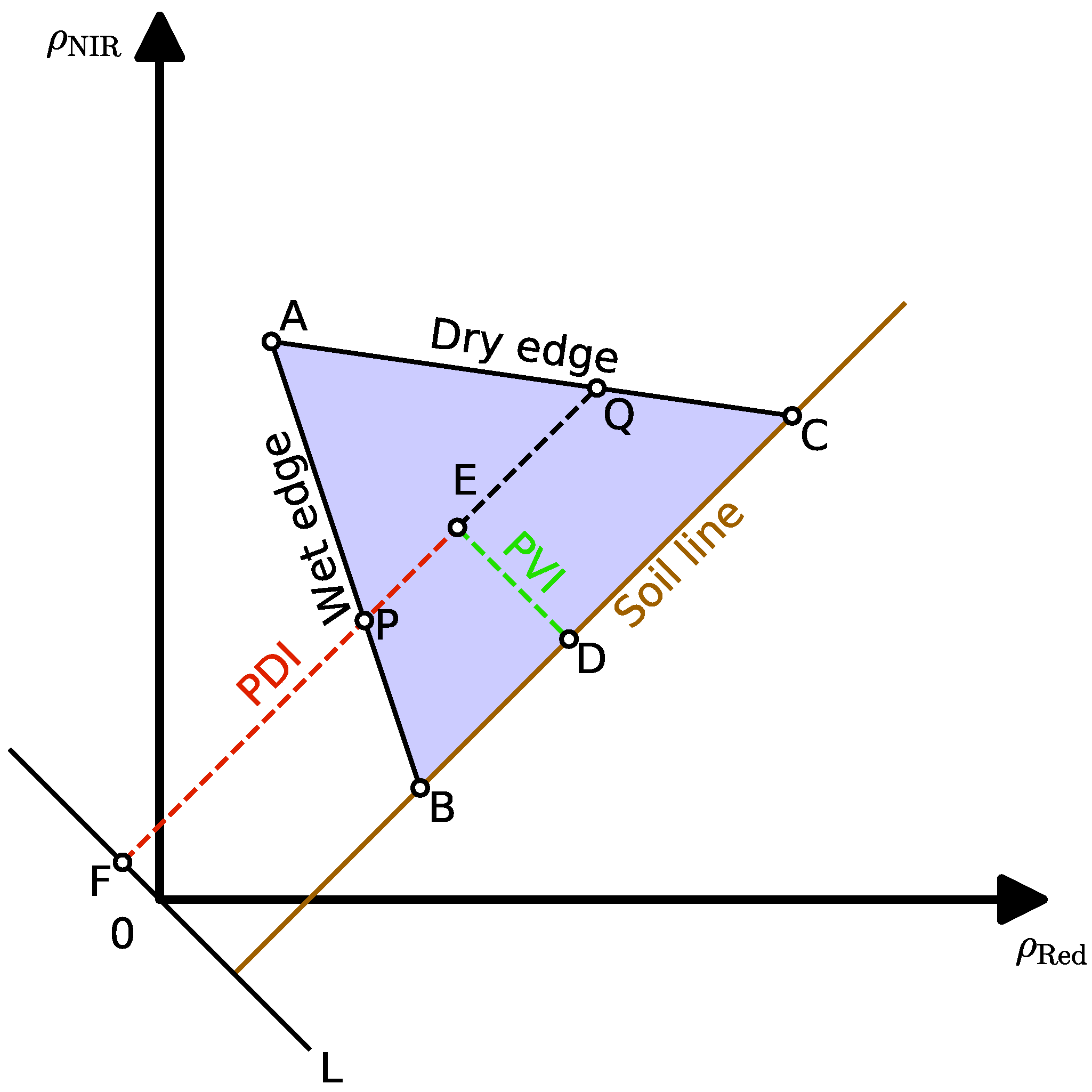
| Perpendicular Vegetation Index (PVI) | M and I are the slope and interception of the soil line in the NIR-Red reflectance space | 1977 [73] | ||
| Soil Adjusted Vegetation Index (SAVI) | L is an empirical coefficient | 1988 [68] | Kenya [99] | |
| Moisture Stress Index (MSI) | 1989 [49] | Morocco [100], India [101] | ||
| Vegetation Condition Index (VCI) | is the historical minimum NDVI value for a specific location, while is the historical maximum NDVI value for the same location | 1990 [61] | U.S. [65,102], China [64,66,67], South Korea [103] | |
| Atmospherically Resistant Vegetation Index (ARVI) | is an empirical coefficient | 1992 [69] | Poland [98] | |
| Anomaly Vegetation Index (AVI) | is the multi-year average of NDVI for a given location in a specific month | 1994 [62] | China [104] | |
| Enhanced Vegetation Index (EVI) | G, , and L are empirical coeifficents | 1995 [70] | East Asia [105] | |
| Normalized Difference Water Index (NDWI) | 1996 [57] | India [106], Morocco [100] | ||
| Photochemical Reflectance Index (PRI) | There are other wavelength selections | 1997 [58] | Bolivia [107], Spain [108], China [109,110] | |
| Simple Ratio Water Index (SRWI) | 2001 [50] | Brazil [111] | ||
| Standardized Vegetation Index (SVI) | is the standard deviation of multi-year NDVI for a given location at a specific time of year. | 2002 [63] | U.S. [63], South Korea [103] | |
| Shortwave Infrared Water Stress Index (SIWSI), also known as the Normalized Difference Infrared Index (NDII) | The SWIR band can be MODIS band 5 or 6 | 2003 [59] | China [112] | |
| Normalized Multiband Drought Index (NMDI) | 2007 [60] | Jordan [113] | ||
| Perpendicular Drought Index (PDI) | M is the slope of the soil line in the NIR-Red reflectance space | 2007 [75] | Iran [114,115], China [116] | |
| Modified Perpendicular Drought Index (MPDI) | FVC is the fractional vegetation cover, and is the PDI value calculated for fully covered vegetation. | 2007 [76] | Iran [114,115], China [116,117] | |
| Shortwave Infrared Perpendicular Water Stress Index (SPSI) | M is the slope of the soil line in the NIR-SWIR reflectance space | 2007 [82] | China [112] | |
| Two-band Enhanced Vegetation Index (EVI2) | G and C are empirical coefficients | 2008 [71] | China [118] | |
| Vegetation Water Stress Index (VWSI) | G is the point of the pixel in the NIR-SWIR space, and EF is the parallel line of the base soil line that crosses G, which intersects the wet edge at E and the dry edge at F (see Figure 4 in [83]). | 2008 [83] | India [119] | |
| Visible and Shortwave Infrared Drought Index (VSDI) | 2013 [51] | Jordan [113], Iraq [120], China [104] | ||
| Modified Shortwave Infrared Perpendicular Water Stress Index (MSPSI) | ; ; M is the slope of the soil line in the - space | 2013 [89] | China [89] | |
| Second Modified Perpendicular Drought Index (MPDI1) | 2013 [78] | China [78] | ||
| Inverted Difference Vegetation Index (IDVI) | 2018 [72] | |||
| Ratio Dryness Monitoring Index (RDMI) | P is the point of the pixel in the NIR-Red space, and DE is the parallel line of the base soil line that crosses P, which intersects the wet edge at D and the dry edge at E (see Figure 8 in [79]). | 2019 [79] | China [79] |
| Mission | Sensor | Time Range | References |
|---|---|---|---|
| Greenhouse gases Observing SATellite (GOSAT) | Thermal And Near-infrared Sensor for carbon Observation Fourier Transform Spectrometer (TANSO-FTS) | 2009–Now | [142,143] |
| GOSAT-2 | TANSO-FTS/2 | 2018–Now | [144] |
| Meteorological Operational satellite (MetOp) | Global Ozone Monitoring Experiment-2 (GOME-2) | 2006–Now (MetOp-A); 2012–Now (MetOp-B); 2018–Now (MetOp-C) | [145,146,147] |
| Environmental Satellite (EnviSat) | SCanning Imaging Absorption spectroMeter for Atmospheric CHartographY (SCIAMACHY) | 2002–2012 | [146,147] |
| MEdium Resolution Imaging Spectrometer (MERIS) | |||
| Orbiting Carbon Observatory (OCO-2) | Orbiting Carbon Observatory (OCO) | 2014–Now | [148] |
| Sentinel-5 Precursor (S-5P) | TROPOspheric Monitoring Instrument (TROPOMI) | 2017–Now | [149] |
| Carbon Dioxide Observation Satellite (TanSat) | Atmospheric Carbon dioxide Grating Spectrometer (ACGS) | 2016–Now | [150,151,152] |
| FLuorescence EXplorer (FLEX) | FLuORescence Imaging Spectrometer (FLORIS) | 2024 (Planned) | [153,154] |
| Index | Expression | Notes | Year Introduced | Applications |
|---|---|---|---|---|
| Apparent Thermal Inertia (ATI) | C is a constant coefficient, is the surface albedo, and and are day/night LST | 1985 [171] | China [192], Thailand [165] | |
| Normalized Difference Temperature Index (NDTI) | is the LST when the composite surface resistance is infinity and the evapotranspiration (ET) is zero, is actual LST, and is the LST when is zero and the ET is equal to the potential ET | 1992 [188] | Australia [187] | |
| Temperature Condition Index (TCI) | T is the smoothed weekly temperature, and and are the multi-year maximum and minimum | 1995 [102] | U.S. [102] | |
| Temperature Rise Index (TRI) | is the average value for a compositing period, and and are the maximum and minimum for the same period among multiple years | 2020 [191] | Australia [191] |
| Index | Expression | Notes | Year Introduced | Applications |
|---|---|---|---|---|
| Vegetation Supply Water Index (VSWI) | 1990 [202] | China [204], Brazil [205,206] | ||
| Vegetation Health Index (VHI) | is an empirical coefficient | 1995 [102] | U.S. [102,186,207], Indonesia [228], Euro-Mediterranean [183], Ethiopia [229] | |
| Vegetation Temperature Condition Index (VTCI) | and represent the maximum and minimum LST of pixels with the same NDVI value | 2001 [194] | China [194,230], India [197] | |
| Temperature Vegetation Drought Index (TVDI) | a and b are fitting coefficients of and NDVI | 2002 [218] | Senegal [218], China [231], Turkmenistan [232] | |
| Improved TVDI (iTVDI) | is the difference between LST and the surface air temperature | 2012 [224] | Iran [224] | |
| Microwave TVDI (MTVDI) | MNDVI is the Microwave NDVI calculated from the Microwave Polarization Difference Index (MPDI), and are fitting coefficients of LST and MNDVI, and and are fitting coefficients of LST and MNDVI; there is also iMTVDI which is similar to iTVDI | 2017 [225] | China [225] | |
| Temperature Fluorescence Drought Index (TFDI) | and are fitting coefficients of LST and SIF, and and are fitting coefficients of LST and SIF | 2020 [226] | China [226] |
Publisher’s Note: MDPI stays neutral with regard to jurisdictional claims in published maps and institutional affiliations. |
© 2021 by the authors. Licensee MDPI, Basel, Switzerland. This article is an open access article distributed under the terms and conditions of the Creative Commons Attribution (CC BY) license (https://creativecommons.org/licenses/by/4.0/).
Share and Cite
Qin, Q.; Wu, Z.; Zhang, T.; Sagan, V.; Zhang, Z.; Zhang, Y.; Zhang, C.; Ren, H.; Sun, Y.; Xu, W.; et al. Optical and Thermal Remote Sensing for Monitoring Agricultural Drought. Remote Sens. 2021, 13, 5092. https://doi.org/10.3390/rs13245092
Qin Q, Wu Z, Zhang T, Sagan V, Zhang Z, Zhang Y, Zhang C, Ren H, Sun Y, Xu W, et al. Optical and Thermal Remote Sensing for Monitoring Agricultural Drought. Remote Sensing. 2021; 13(24):5092. https://doi.org/10.3390/rs13245092
Chicago/Turabian StyleQin, Qiming, Zihua Wu, Tianyuan Zhang, Vasit Sagan, Zhaoxu Zhang, Yao Zhang, Chengye Zhang, Huazhong Ren, Yuanheng Sun, Wei Xu, and et al. 2021. "Optical and Thermal Remote Sensing for Monitoring Agricultural Drought" Remote Sensing 13, no. 24: 5092. https://doi.org/10.3390/rs13245092
APA StyleQin, Q., Wu, Z., Zhang, T., Sagan, V., Zhang, Z., Zhang, Y., Zhang, C., Ren, H., Sun, Y., Xu, W., & Zhao, C. (2021). Optical and Thermal Remote Sensing for Monitoring Agricultural Drought. Remote Sensing, 13(24), 5092. https://doi.org/10.3390/rs13245092