Abstract
Global Navigation Satellite System (GNSS) Precise Point Positioning (PPP) enables the estimation the ionospheric vertical total electron content (VTEC) as well as the by-product of the satellite Pseudorange observable-specific signal bias (OSB). The single-frequency PPP models, with the ionosphere-float and ionosphere-free approaches in ionospheric studies, have recently been discussed by the authors. However, the multi-frequency observations can improve the performances of the ionospheric research compared with the single-frequency approaches. This paper presents three dual-frequency PPP approaches using the BeiDou Navigation Satellite System (BDS) B1I/B3I observations to investigate ionospheric activities. Datasets collected from the globally distributed stations are used to evaluate the performance of the ionospheric modeling with the ionospheric single- and multi-layer mapping functions (MFs), respectively. The characteristics of the estimated ionospheric VTEC and BDS satellite pseudorange OSB are both analyzed. The results indicated that the three dual-frequency PPP models could all be applied to the ionospheric studies, among which the dual-frequency ionosphere-float PPP model exhibits the best performance. The three dual-frequency PPP models all possess the capacity for ionospheric applications in the GNSS community.
1. Introduction
As we all know, a large amount of the free electrons exists in the Earth’s ionosphere. Serving as the significant region of the Earth’s near space, the ionospheric delay is an important error source in satellite PNT services, which can cause the delay of several meters to several hundred meters in the GNSS signal transmission [1,2,3,4,5]. With the rapid development of the GNSS, it has been the most important tool for ionospheric monitoring and correction due to its advantages of all-weather global coverage and high temporal and spatial resolutions. Since the ionosphere is a dispersive medium, the ionospheric delay can be eliminated by multi-frequency observations. Single-frequency GNSS users require external ionospheric information to eliminate the ionospheric delay. One commonly applied way is to use the empirical models such as the Klobuchar, NeQuick, BDGIM, NTCM and so on [6,7,8,9,10]. Another alternative way is to apply the ionospheric TEC map obtained from the globally distributed stations.
The ways to extract the ionospheric STEC include the CCL and PPP [11,12]. CCL is known as the most convenient method in the ionospheric community, entailing a process of smoothing the pseudorange with the carrier phase observation, whose accuracy and reliability can be affected by the smoothing error, multipath effect and receiver DCB intra-day variation [13,14]. When the number of the continuous epoch observations is sufficient, the noise effect of the the pseudorange observations will be significantly reduced, whereas the error caused by multipath cannot be eliminated. MCCL is an alternative, simple and efficient method to estimate the ionospheric delay, in which the effect of the receiver DCB intra-day variation can be avoided [15,16]. Similarly, the multi-frequency PPP can also overcome the disadvantages of the traditional approaches. The DFPPP1 approach proposed by Zhang et al. [14] is the typical method for extracting the ionospheric STEC, in which the STEC observations and multipath is reduced by more than 70% compared to the CCL approach. Tu el al. [17] also validated that the DFPPP1 approach in a real-time scenario can be applied for the ionospheric study, in which the accuracy of the estimated VTEC and satellite DCB is 1–2 TECU and 0.4 ns, respectively. Zhang et al. [18] modified and improved the DFPPP1 approach to estimate the slant ionospheric observables, in which the receiver pseudorange bias is considered as the time-varying parameter. Liu et al. [11] applied the multi-GNSS multi-frequency ionosphere-float approach for the ionospheric modeling. PPP has obvious advantages over the ionospheric observable extraction compared to the CCL. The ionospheric STEC extracted from PPP is consistent with that from the CCL method but with higher accuracy. The two methods have been widely applied in the ionospheric modeling [11,19,20,21].
Regarding the above literatures, the MF used in ionospheric VTEC modeling is based on the Earth ionospheric single-layer assumption. However, the influence of ionospheric single-layer MF may cause larger errors in the vertical direction due to the effect of ionospheric horizontal gradient and equilibrium condition deviation [22]. Hence, the ionospheric height is an important factor in the ionospheric MF [23,24]. Hoque and Jakowski [25] proposed the ionospheric multi-layer MF to describe the ionospheric vertical structure, in which the ionospheric projected error can be reduced by more than 50%. Thus, applying the ionospheric multi-layer MF is an effective way to improve the accuracy of ionospheric modeling.
Su and Jin [26] has discussed the applications of the two single-frequency PPP models for the ionospheric study. However, the multi-frequency observations can improve the performances of the ionospheric modeling when compared with the single-frequency approaches. With a view to extend this work, this study presents three dual-frequency PPP models to investigate the ionospheric and hardware delay performance. The previously mentioned literature only concentrated on the ionosphere-float PPP solution for the ionospheric study. The comparison of this study can help the readers better understand the state-of-the-art approach for the ionospheric research and improve the real-time ionospheric services in the GNSS community [27]. The pseudorange OSB is estimated by viewing the undifferenced format of the DCB, which is more straightforward and directly applicable to the original GNSS measurements [28]. The three models provide alternatives for the pseudoraneg OSB estimation. The experimental data and analytical performance are introduced. Finally, the conclusions are given.
2. Methods
In this section, we begin with the BDS general observation model. Then, three dual-frequency methods are discussed with respect to the extracted ionospheric observables. The approaches for the estimated ionospheric VTEC and satellite pseudorange OSB are also discussed.
2.1. General Observations
The BDS raw observations for the satellite s with regard to the receiver r at epoch t read [29]:
where and denote the carrier phase and pseudorange observables; denotes the satellite and receiver geometrical range; and denote the receiver and satellite clock offsets; denotes the affected tropospheric delay; denotes the slant ionospheric delay with respect to the BDS first frequency; is the frequency-dependent multiplier factor, where denotes the jth frequency; and denote the pseudorange instrumental delays for the receiver and satellite, respectively; and denote the corresponding carrier phase instrumental delays; denotes the ambiguity parameter; and denote the pseudorange and carrier phase measurement noise, including multipath, respectively.
2.2. DFPPP1: Dual-Frequency Ionosphere-Float PPP Model
We define the dual-frequency ionosphere-float PPP as DFPPP1 model here. With m observed satellites tracking the signals on ith and jth frequencies, the DFPPP1 model is written as [21]:
where
- , denotes the tropospheric zenith wet delay (ZWD), denotes the receiver clock offset, , ;
- denotes m-dimension row vector, in which all values are 1;
- denotes m-dimension identity matrix;
- denotes the design matrix of the tropospheric wet mapping function;
- ; ; ;
- , in which denotes the ratio of the observation noise on ith frequency.
- denotes the corresponding observation precision matrix in the vertical direction, and denotes the elevation diversity cofactor matrix;
- denotes the Kronecker product.
The corresponding estimated parameters read:
2.3. DFPPP2: Dual-Frequency Ionosphere-Free PPP Model
With m observed satellites tracking the signals on ith and jth frequencies, the DFPPP2 model is written as [30]:
where
, , in which
The corresponding estimated parameters read:
The wide-lane ambiguity can be represented by the wide-lane carrier phase observables and narrow-lane pseudorange observables, which reads:
with
Thereafter, the ionospheric ambiguity can be represented by the wide-lane ambiguity and ionospheric ambiguity in PPP, which reads:
Then, we can obtain the ionospheric observables as:
Considering that the raw pseudorange observations have a higher noise, we apply the Hatch filter to smooth the observations by the carrier phase observations [31,32]. The sharp variation in the pseudorange observation that affect the leveling is checked and removed [33].
2.4. DFPPP3: Dual-Frequency UofC PPP Model
With m observed satellites tracking the signals on ith and jth frequencies, the DFPPP3 model is written as [34]:
where
The corresponding estimated parameters read:
Then, the ionospheric ambiguity can be combined by two estimated ambiguities in DFPPP3 model, which can be expressed as:
Similar to DFPPP2 solution, we can obtain the ionospheric observables as well.
2.5. Ionospheric Modeling and OSB Estimation
As we can see, the ionospheric delays estimated from the DFPPP1, DFPPP2 and DFPPP3 models have the identical forms. The ionospheric observables can be viewed as the linear relationship of the STEC and SPR DCB [35]. To build the link of the STEC and VTEC, the ionospheric MF is usually established according to the satellite elevation. The single-layer MF can be expressed as [36]:
where denotes coefficient of the single-layer MF model, of which the SLM is 1 and MSLM is 0.9782. and denote the mean Radius Earth and IPP height. The IPP height is set as the 450 km.
The multi-layer MF assumes that the ionosphere is composed of numerous thin shells. The obliquity factors, manifesting the link of the corresponding VTEC and the incremental STEC , can be written as [25]:
where denotes the peak ionization height and denotes the atmospheric scale height.
The GTSF is applied to estimate the ionospheric VTEC values and reads [37]:
where and are the IPP latitude and receiver geographical latitude, respectively.
In the station-based local ionospheric modeling, the ionospheric observable weight is applied by considering the local time satellite elevation effect and expressed as:
where p denotes the weight of the ionospheric observable.
To avoid the singularity of the equation, the constraints are introduced and read:
Then, the ionospheric VTEC can be isolated and the satellite OSB can be estimated.
2.6. Analysis of PPP Approaches
Table 1 compares the three dual-frequency PPP approaches in the observations and parameter fields. The degrees of freedom for the three PPP models are the same. The DFPPP1 model directly estimates the ionospheric delay as the unknown parameters. The ionospheric observables extracted by the DFPPP2 approach are influenced by the code and leveling errors. The ionospheric observables estimated in DFPPP3 method are affected by the carrier phase noises. Theoretically, the ionospheric observables from the DFPPP1 and DFPPP3 model are more accurate than that from the DFPPP2 approach.

Table 1.
Comparison of three dual-frequency PPP approaches.
3. Results and Analysis
3.1. Data Processing Strategy
We selected 77 stations from the MGEX network in October 2020 to analyze the experimental performance. All of the stations can track the BDS-2 and BDS-3 B1I/B3I signals. The DFPPP1, DFPPP2 and DFPPP3 models are all conducted. Figure 1 depicts the distribution of the MGEX stations. The precise clock and orbit products provided by the GFZ analysis center are applied for the PPP data processing. Moreover, we utilized the forward and backward Kalman filter to avoid the effect of the unconverging ambiguities. The elevation cutoff of satellites in PPP is 7.5° and the elevation cutoff for the ionospheric VTEC modeling is 20° [38]. The random walk noise for the ionospheric delay is 10−4 m2/s in DFPPP1 solution. The ionospheric single- and multi-layer MFs are both applied to evaluate the experimental performance. Other error items in the data processing strategies can refer to Su et al. [39].
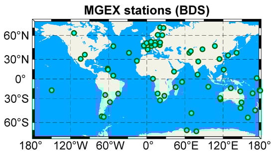
Figure 1.
Distribution of the selected MGEX stations.
3.2. Analysis of the Ionospheric Observables from PPP
Figure 2 depicts the slant ionospheric delay estimated from one randomly selected station ULAB with three dual-frequency PPP models. The extracted slant ionospheric delay contains the pure slant ionospheric delay and SPR DCB. As we can see, the variation tendency of the ionospheric observables from three models are generally consistent with each other. For further analysis and understanding, we put the slant ionospheric delay from different PPP models together. Figure 3 shows the estimated slant ionospheric delay with the elevation for the BDS C26 satellite with the three PPP models. The results indicate that the extracted ionospheric observables from the three models have generally overlapped with each other, which proves the consistency of the ionospheric observables from three models. Using the slant ionospheric observables from the DFPPP1 model as the datum, we calculate the ionospheric observables difference STD for the remaining two PPP models.
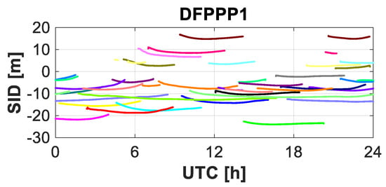
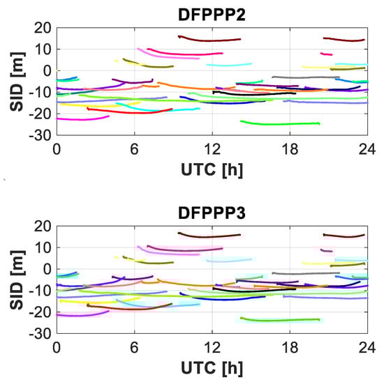
Figure 2.
Slant ionospheric delay at station ULAB with the DFPPP1, DFPPP2 and DFPPP3 models on DOY 288, 2020.
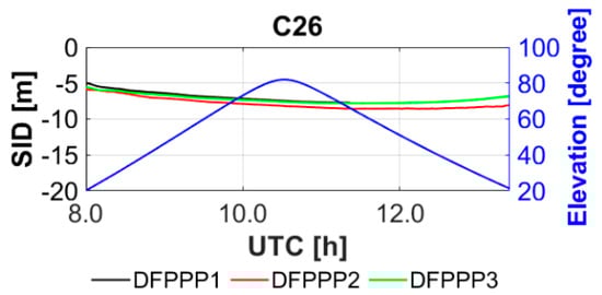
Figure 3.
Slant ionospheric delay with the elevation variation with the DFPPP1, DFPPP2 and DFPPP3 models.
Figure 4 shows the STD distribution for the DFPPP2 and DFPPP3 models with regard to the slant ionospheric observables. The STD of the ionospheric observables difference is able to reflect the smoothing leveling of the ionospheric observables. We can see that the higher consistency exists in the ionospheric observables of the DFPPP1 and DFPPP3 models. The mean values of the STD for the ionospheric observables difference with the DFPPP2 and DFPPP3 models are 0.65 and 0.09 m, respectively, with respect to the DFPPP1 model. The leveling error and pseudorange noises lead to the higher noise in the DFPPP2 model. The DFPPP1 and DFPPP3 models are capable of estimating slant ionospheric delay with the centimeter-level accuracy.
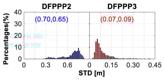
Figure 4.
STD distribution of ionospheric observables differences for the DFPPP2 and DFPPP3 models. The corresponding medium and mean values are also shown.
The effect of the pure ionospheric observables and satellite DCB can be eliminated when differencing the ionospheric observables of the stations on short- or zero-baselines. Based on this, the ionospheric observable leveling noise magnitude can be evaluated. Figure 5 shows the slant ionospheric delay difference for the two stations WTZZ and WTZS with three dual-frequency PPP models. The STDs of the single-difference ionospheric observables are 0.06, 0.13 and 0.11 m, respectively, for the DFPPP1, DFPPP2 and DFPPP3 models. The ionospheric observables of the three PPP models are in the level of sub-meter and the DFPPP1 model estimates the ionospheric observables with the highest accuracy.
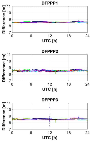
Figure 5.
Slant ionospheric delay single difference for the short-baseline stations with the DFPPP1, DFPPP2 and DFPPP3 models.
We selected five short baseline stations to analyze the ionospheric leveling error [26]. Figure 6 depicts the average STD of the slant ionospheric delay single difference with the DFPPP1, DFPPP2 and DFPPP3 models. We can see that the ionospheric delay single differences range from the 0.03 to 0.25 m. For the three PPP models, the leveling error of the DFPPP2 model is obviously larger than DFPPP3 and the DFPPP1 model exhibits the slowest noise.
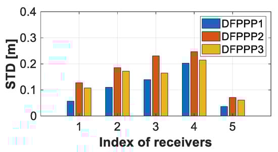
Figure 6.
Average values of the ionospheric delay single difference STDs with the DFPPP1, DFPPP2 and DFPPP3 models.
3.3. Analysis of the Estimated VTEC
The ionospheric single- and multi-layer MFs are both adopted to estimated VTEC. To better analyze and evaluate the corresponding reliability, Figure 7 shows the estimated ionospheric VTEC for six random selected stations with the DFPPP1, DFPPP2 and DFPPP3 models. The VTEC values from the IGS GIM values are also used for comparison, whose accuracy is 2–8 TECU [40]. The corresponding VTEC accuracy varies from the 0.4 to 3.4 TECU.
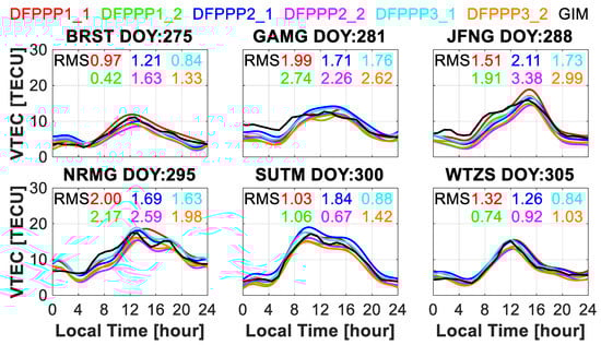
Figure 7.
Estimated ionospheric VTEC for the six stations with the DFPPP1, DFPPP2 and DFPPP3 models.
For further discussion, Figure 8 shows the time series of the estimated ionospheric VTEC with the ionospheric single- and multi-layer MFs for the two short-baseline stations on three days with the DFPPP1, DFPPP2 and DFPPP3 models. The ionospheric VTEC values can theoretically be considered as the same value. The ionospheric single-layer MF estimated ionospheric VTEC is more consistent with the VTEC value from the GIM, owing to the same MF in which they both applied by neglecting the ionospheric horizontal gradient [41]. Figure 9 depicts the estimated ionospheric VTEC single-difference for the two short-baseline stations with the DFPPP1, DFPPP2 and DFPPP3 models. The RMS of the ionospheric observable single difference is shown to reflect the precision of the ionospheric delay with the corresponding method. By applying the multi-layer MF, the precision of the estimated ionospheric VTEC is improved.
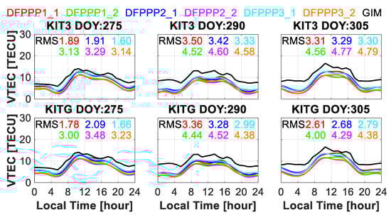
Figure 8.
Estimated ionospheric VTEC for the two short-baseline stations with the DFPPP1, DFPPP2 and DFPPP3 models.
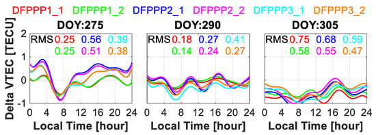
Figure 9.
Estimated ionospheric VTEC single-difference for the two short-baseline stations with the DFPPP1, DFPPP2 and DFPPP3 models.
With the GIM product as the reference, Figure 10 shows the distribution of the RMS, mean bias and STD of the ionospheric VTEC difference for the three PPP models. The VTEC accuracy with different approaches is approximately 2 TECU. The ionospheric VTEC value estimated with the single-layer solution is larger than the multi-layer as a whole. Faint difference can be found within the corresponding RMS and STD values.
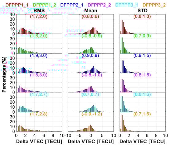
Figure 10.
Distribution of the RMS, mean bias and STD of the ionospheric VTEC difference for the three PPP models and IGS GIM values.
Moreover, Figure 11 depicts the distribution of the RMS, mean bias and STD of the ionospheric VTEC difference of the DFPPP2 and DFPPP3 models by using the DFPPP1 model as the reference. The results indicate that the accuracy of the ionospheric VTEC value estimated with the multi-layer MF is better. The ionospheric observables derived with the DFPPP3 models exhibit the higher consistency than the DFPPP2 model. The median RMS errors of the ionospheric VTEC are 1.0, 0.9, 0.7 and 0.7 TECU for the DFPPP2 and DFPPP3 models with two MFs.
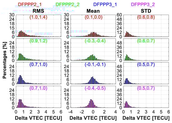
Figure 11.
Distribution of the RMS, mean bias and STD of the ionospheric VTEC difference for the DFPPP2 and DFPPP3 models compared with the DFPPP1 model.
Figure 12 shows the RMS distribution of the ionospheric VTEC difference for the short-baseline stations with two MFs by the DFPPP1, DFPPP2 and DFPP3 models. We can also find the similar conclusion. For instance, the average RMS of the ionospheric VTEC difference decrease from the (0.45, 0.47, 0.29, 0.52, 0.43) TECU to (0.39, 0.40, 0.25, 0.45, 0.36) TECU after using the ionospheric multi-layer MF. The accuracy of the ionospheric VTEC from the DFPPP2 model is relatively poorer. The results of five short-baseline stations prove that the ionospheric VTEC can achieve the accuracy of the centimeter level.
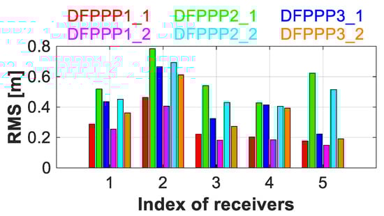
Figure 12.
RMS distribution of the ionospheric VTEC difference for the short-baseline stations for the three PPP models.
3.4. Analysis of the Estimated BDS Satellite Pseudorange OSB
To evaluate the performance of the estimated BDS C2I and C6I satellite pseudorange OSB with three PPP models, we analyze the pseudorange OSB values for the whole month. Firstly, the slant ionospheric observables are extracted from the PPP models. Then, the BDS satellite pseudorange OSB values are estimated from the ionospheric observables. The satellite pseudorange OSB values are analyzed and validated in terms of the stability and consistency in this section.
Figure 13 depicts the time series of the estimated pseudorange OSB by the DFPPP1, DFPPP2 and DFPPP3 models in October 2020. The estimated satellite pseudorange OSB values in different days may be inconsistent with the zero-mean constraint by different observed satellites, which will lead to systematic changes in the corresponding satellite pseudorange OSB solutions in different days. Hence, we convert the satellite pseudorange OSB obtained during all days to the same datum. It can be seen from the figure that the BDS satellite OSB time series estimated by three PPP models is basically continuous and stable, whereas a small number of BDS satellites will jump in part of the days. For example, BDS C45 satellite shifts several nanoseconds at DOY 288, 2020. For the three PPP models, the satellite pseudorange OSB estimated by the ionospheric single- and multi-layer MFs is basically consistent, that is to say, different MFs have little influence on the satellite pseudorange OSB [39]. The variation of satellite pseudorange OSB time series estimated by the three PPP models is basically the same. The present PPP models all can effectively estimate the satellite pseudorange OSB values.
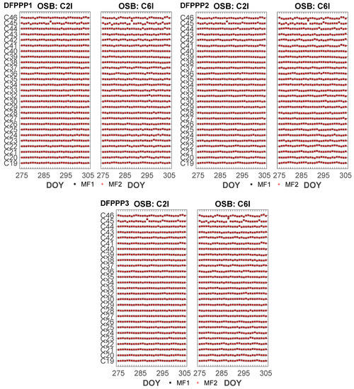
Figure 13.
Estimated BDS pseudorange OSB with two MFs by the DFPPP1, DFPPP2 and DFPPP3 models.
To analyze the stability of the estimated BDS satellites pseudorange OSB, the monthly average and STD values of the estimated BDS pseudorange OSB values by the DFPPP1, DFPPP2 and DFPPP3 models in October 2020 are shown in Figure 14 and Figure 15. We can see that the monthly mean values of BDS satellite pseudorange OSB have a wide distribution, ranging from −90 ns to 150 ns. With respect to the pseudorange OSB stability, the STD values of BDS satellite pseudorange OSB are less than 1 ns except for the GEO satellites. The STDs of the BDS satellite pseudorange OSB with three PPP models are at the same level. The BDS satellite pseudorange OSB estimated with the DFPPP1 model exhibits the lowest STD, indicating that the corresponding OSB time series are the most stable. Owing to the introduced zero-mean condition, the ratio of the corresponding values of BDS satellites C2I and C6I pseudorange OSB value is . For BDS C45 and C46 satellites, the pseudorange OSB stability is poorer than other satellites due to the influence of observation quality and instability.
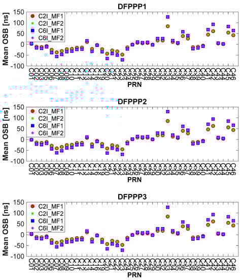
Figure 14.
Average value of the estimated BDS pseudorange OSB by the DFPPP1, DFPPP2 and DFPPP3 models on October 2020.
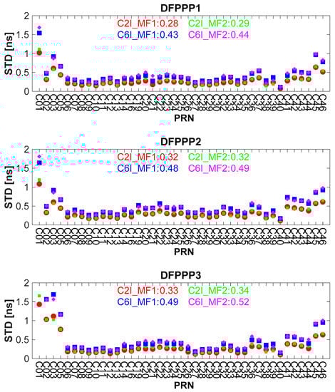
Figure 15.
Monthly STD value of the estimated BDS pseudorange OSB by the DFPPP1, DFPPP2 and DFPPP3 models in October 2020. The average STD values are also shown in the figure.
Figure 16 shows the monthly RMS error of the estimated BDS C2I and C6I pseudorange OSB with two MFs by the DFPPP1, DFPPP2 and DFPPP3 models in October 2020 compared with the CAS satellite pseudorange OSB product. The average RMS error of the GEO, IGSO, MEO and all BDS satellites are also shown. The accuracy of BDS GEO satellite pseudorange OSB is 2–3 times less than that of IGSO among the BDS satellites. Due to the poor accuracy of C45 and C46 satellites, the average RMS of MEO satellites is higher than that of IGSO satellites on the whole. It is unsurprising that the some of the BDS-3 satellites are still in the testing and improvement as the latest satellite navigation system fully deployed. For the three PPP models, the RMS error of the satellite pseudorange OSB is (0.34, 0.35, 0.52, 0.54) ns for the DFPPP1 model. The RMS error of the satellite pseudorange OSB is (0.40, 0.41, 0.60, 0.61) ns for the DFPPP2 model. The RMS error of the satellite pseudorange OSB is (0.37, 0.39, 0.57, 0.59) ns for the DFPPP3 model. The BDS satellite pseudorange OSB estimated by different PPP models has high flexibility and reliable accuracy.
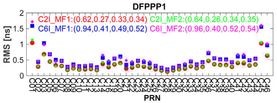
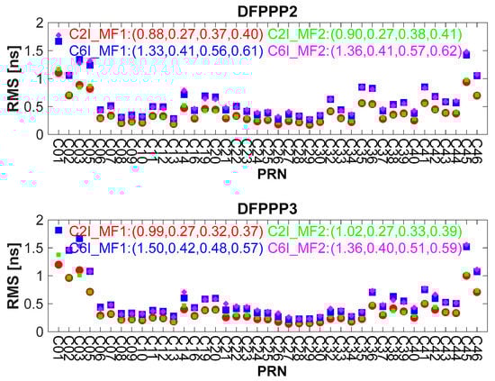
Figure 16.
Monthly RMS error value of the estimated BDS pseudorange OSB by the DFPPP1, DFPPP2 and DFPPP3 models in October 2020 compared to the CAS product. The average RMS errors of the GEO, IGSO, MEO and all BDS satellites are also shown.
4. Conclusions
In this study, three dual-frequency PPP models, namely DFPPP1, DFPPP2 and DFPPP3 models are presented for ionospheric studies. The mathematical models of the dual-frequency PPP models are introduced in detail. Datasets collected from the MGEX network are used to evaluate the performance of the estimated slant ionospheric observables, VTEC and satellite pseudorange OSB. The following conclusions are derived.
Firstly, the ionospheric observables from the three PPP models are in the level of sub-meter and the DFPPP1 model estimates the highest accuracy ionospheric observables. The leveling error of the DFPPP2 model is obviously larger than DFPPP3 model and the DFPPP1 model exhibits the slowest noise.
Secondly, the RMS error of the VTEC is approximately 2 TECU with respect to the GIM product. The accuracy of the ionospheric VTEC value estimated with the ionospheric multi-layer MF is higher. The ionospheric observables derived with the DFPPP3 models exhibits a higher consistency than the DFPPP1 model. The ionospheric VTEC can achieve the accuracy of the centimeter level.
Thirdly, the variation in satellite pseudorange OSB time series estimated by the three PPP models is basically the same. The present PPP models can all effectively estimate the satellite pseudorange OSB values. The partial BDS satellite pseudorange OSB stability is poor due to the influence of observation quality and instability. The RMS error of the satellite pseudorange OSB is in the level of sub-nanosecond. The accuracy of BDS GEO satellite pseudorange OSB is 2–3 times less than that of IGSO among the BDS satellites. Due to the poor accuracy of C45 and C46 satellites, the average RMS of MEO satellites is higher than that of the IGSO satellites on the whole. The BDS satellite pseudorange OSB estimated by different the PPP models has high flexibility and reliable accuracy.
In summary, the three PPP models can all be applied for the ionospheric studies. It is recommended that the DFPPP1 and DFPPP3 models are used for the corresponding performance is relatively reliable.
Author Contributions
K.S. and S.J. designed the experiment; K.S. performed and analyzed the experiment and wrote the paper. S.J. helped in revision and discussion. All authors have read and agreed to the published version of the manuscript.
Funding
This work was supported National Natural Science Foundation of China Project (Grant No. 12073012), National Natural Science Foundation of China-German Science Foundation Project (Grant No. 41761134092).
Data Availability Statement
The applied datasets are collected from the IGS.
Acknowledgments
The authors acknowledged that the GNSS data were obtained from the IGS and the precise clock and orbit products are provided by the GFZ.
Conflicts of Interest
The authors declare no conflict of interest.
Abbreviation
| BDGIM | BeiDou Global Ionospheric delay correction Model |
| BDS | Beidou Navigation Satellite System |
| CCL | Carrier-to-Code Leveling |
| DCB | Differential Code Bias |
| DFPPP1 | Dual-frequency ionosphere-float PPP |
| DFPPP2 | Dual-frequency ionosphere-free PPP |
| DFPPP3 | Dual-frequency UofC PPP |
| DOY | Day Of Year |
| GEO | Geostationary Earth Orbit |
| GFZ | Deutsches GeoForschungsZentrum |
| GIM | Global Ionospheric Map |
| GNSS | Global Navigation Satellite System |
| GTSF | Generalized Trigonometric Series Function |
| IGS | International GNSS Service |
| IGSO | Inclined GeoSynchronous Orbit |
| IPP | Ionospheric Pierce Point |
| MCCL | Modified Carrier-to-Code Leveling |
| MEO | Medium Earth Orbit |
| MF | Mapping Function |
| MGEX | Multi-GNSS EXperiment |
| MSLM | Modified Single-Layer Model |
| NTCM | Neustrelitz TEC Model |
| OSB | Observable-specific Signal Bias |
| PNT | Positioning, Navigation and Timing |
| PPP | Precise Point Positioning |
| RMS | Root Mean Square |
| SLM | Single-Layer Model |
| SPR | Satellite Plus Receiver |
| STEC | Slant Total Electron Content |
| STD | STandard Deviation |
| TEC | Total Electron Content |
| TECU | Total Electron Content Unit |
| VTEC | Vertical Total Electron Content |
References
- Hoque, M.; Jakowski, N. A new global model for the ionospheric F2 peak height for radio wave propagation. Ann. Geophys. 2012, 30, 797–809. [Google Scholar] [CrossRef] [Green Version]
- Jin, S.; Su, K. PPP models and performances from single-to quad-frequency BDS observations. Satell. Navig. 2020, 1, 16. [Google Scholar] [CrossRef]
- Yang, Y.; Mao, Y.; Sun, B. Basic performance and future developments of BeiDou global navigation satellite system. Satell. Navig. 2020, 1, 1. [Google Scholar] [CrossRef] [Green Version]
- Jin, S.; Jin, R.; Kutoglu, H. Positive and negative ionospheric responses to the March 2015 geomagnetic storm from BDS observations. J. Geod. 2017, 91, 613–626. [Google Scholar] [CrossRef]
- Anđić, D. Impact of sampling interval on variance components of epoch-wise residual error in relative GPS positioning: A case study of a 40-km-long baseline. Geod. Geodyn. 2021, 12, 368–380. [Google Scholar] [CrossRef]
- Hoque, M.; Jakowski, N. An alternative ionospheric correction model for global navigation satellite systems. J. Geod. 2015, 89, 391–406. [Google Scholar] [CrossRef]
- Klobuchar, J.A. Ionospheric time-delay algorithm for single-frequency GPS users. IEEE Trans. Aerosp. Electron. Syst. 1987, AES-23, 325–331. [Google Scholar] [CrossRef]
- Nava, B.; Coisson, P.; Radicella, S. A new version of the NeQuick ionosphere electron density model. J. Atmos. Sol. Terr. Phys. 2008, 70, 1856–1862. [Google Scholar] [CrossRef]
- Yuan, Y.; Wang, N.; Li, Z.; Huo, X. The BeiDou global broadcast ionospheric delay correction model (BDGIM) and its preliminary performance evaluation results. Navigation 2019, 66, 55–69. [Google Scholar] [CrossRef] [Green Version]
- Jin, S.; Han, L.; Cho, J. Lower atmospheric anomalies following the 2008 Wenchuan Earthquake observed by GPS measurements. J. Atmos. Sol. Terr. Phys. 2011, 73, 810–814. [Google Scholar] [CrossRef]
- Liu, T.; Zhang, B.; Yuan, Y.; Zhang, X. On the application of the raw-observation-based PPP to global ionosphere VTEC modeling: An advantage demonstration in the multi-frequency and multi-GNSS context. J. Geod. 2020, 94, 1. [Google Scholar] [CrossRef]
- Psychas, D.; Verhagen, S.; Liu, X.; Memarzadeh, Y.; Visser, H. Assessment of ionospheric corrections for PPP-RTK using regional ionosphere modelling. Meas. Sci. Technol. 2018, 30, 014001. [Google Scholar] [CrossRef] [Green Version]
- Chen, L.; Yi, W.; Song, W.; Shi, C.; Lou, Y.; Cao, C. Evaluation of three ionospheric delay computation methods for ground-based GNSS receivers. GPS Solut. 2018, 22, 125. [Google Scholar] [CrossRef]
- Ciraolo, L.; Azpilicueta, F.; Brunini, C.; Meza, A.; Radicella, S. Calibration errors on experimental slant total electron content (TEC) determined with GPS. J. Geod. 2007, 81, 111–120. [Google Scholar] [CrossRef]
- Zha, J.; Zhang, B.; Yuan, Y.; Zhang, X.; Li, M. Use of modified carrier-to-code leveling to analyze temperature dependence of multi-GNSS receiver DCB and to retrieve ionospheric TEC. GPS Solut. 2019, 23, 103. [Google Scholar] [CrossRef]
- Zhang, B.; Teunissen, P.J.; Yuan, Y.; Zhang, X.; Li, M. A modified carrier-to-code leveling method for retrieving ionospheric observables and detecting short-term temporal variability of receiver differential code biases. J. Geod. 2019, 93, 19–28. [Google Scholar] [CrossRef] [Green Version]
- Tu, R.; Zhang, H.; Ge, M.; Huang, G. A real-time ionospheric model based on GNSS Precise Point Positioning. Adv. Space Res. 2013, 52, 1125–1134. [Google Scholar] [CrossRef]
- Zhang, B.; Zhao, C.; Odolinski, R.; Liu, T. Functional model modification of precise point positioning considering the time-varying code biases of a receiver. Satell. Navig. 2021, 2, 11. [Google Scholar] [CrossRef]
- Li, Z.; Wang, N.; Hernández-Pajares, M.; Yuan, Y.; Krankowski, A.; Liu, A.; Zha, J.; García-Rigo, A.; Roma-Dollase, D.; Yang, H. IGS real-time service for global ionospheric total electron content modeling. J. Geod. 2020, 94, 32. [Google Scholar] [CrossRef]
- Ren, X.; Zhang, X.; Xie, W.; Zhang, K.; Yuan, Y.; Li, X. Global ionospheric modelling using multi-GNSS: BeiDou, Galileo, GLONASS and GPS. Sci. Rep. 2016, 6, 33499. [Google Scholar] [CrossRef] [Green Version]
- Liu, T.; Zhang, B.; Yuan, Y.; Li, M. Real-Time Precise Point Positioning (RTPPP) with raw observations and its application in real-time regional ionospheric VTEC modeling. J. Geod. 2018, 92, 1267–1283. [Google Scholar] [CrossRef]
- Komjathy, A.; Sparks, L.; Mannucci, A.J.; Coster, A. The ionospheric impact of the October 2003 storm event on Wide Area Augmentation System. GPS Solut. 2005, 9, 41–50. [Google Scholar] [CrossRef]
- Li, M.; Yuan, Y.; Zhang, B.; Wang, N.; Li, Z.; Liu, X.; Zhang, X. Determination of the optimized single-layer ionospheric height for electron content measurements over China. J. Geod. 2018, 92, 169–183. [Google Scholar] [CrossRef]
- Xiang, Y.; Gao, Y. An enhanced mapping function with ionospheric varying height. Remote Sens. 2019, 11, 1497. [Google Scholar] [CrossRef] [Green Version]
- Hoque, M.M.; Jakowski, N. Mitigation of ionospheric mapping function error. In Proceedings of the 26th International Technical Meeting of the Satellite Division of The Institute of Navigation (ION GNSS+ 2013), Nashville, TN, USA, 16–20 September 2013. [Google Scholar]
- Su, K.; Jin, S. A novel GNSS single-frequency PPP approach to estimate the ionospheric TEC and satellite pseudorange observable-specific signal bias. IEEE Trans. Geosci. Remote Sens. 2021. [Google Scholar] [CrossRef]
- Li, Z.; Wang, N.; Liu, A.; Yuan, Y.; Wang, L.; Hernández-Pajares, M.; Krankowski, A.; Yuan, H. Status of CAS global ionospheric maps after the maximum of solar cycle 24. Satell. Navig. 2021, 2, 19. [Google Scholar] [CrossRef]
- Wang, N.; Li, Z.; Duan, B.; Hugentobler, U.; Wang, L. GPS and GLONASS observable-specific code bias estimation: Comparison of solutions from the IGS and MGEX networks. J. Geod. 2020, 94, 74. [Google Scholar] [CrossRef]
- Leick, A.; Rapoport, L.; Tatarnikov, D. GPS Satellite Surveying; John Wiley & Sons: Hoboken, NJ, USA, 2015. [Google Scholar]
- Erol, S.; Alkan, R.M.; Ozulu, İ.M.; İlçi, V. Performance analysis of real-time and post-mission kinematic precise point positioning in marine environments. Geod. Geodyn. 2020, 11, 401–410. [Google Scholar] [CrossRef]
- Lee, H.; Rizos, C. Position-domain hatch filter for kinematic differential GPS/GNSS. IEEE Trans. Aerosp. Electron. Syst. 2008, 44, 30–40. [Google Scholar] [CrossRef] [Green Version]
- Dyrud, L.; Jovancevic, A.; Ganguly, S. Ionospheric measurement with GPS: Receiver techniques and methods. In Proceedings of Proceedings of the 20th International Technical Meeting of the Satellite Division of The Institute of Navigation (ION GNSS 2007), Fort Worth, TX, USA, 25–28 September 2007; pp. 2313–2323. [Google Scholar]
- Yasyukevich, Y.; Mylnikova, A.; Vesnin, A. GNSS-based non-negative absolute ionosphere total electron content, its spatial gradients, time derivatives and differential code biases: Bounded-variable least-squares and taylor series. Sensors 2020, 20, 5702. [Google Scholar] [CrossRef]
- Li, B.; Ge, H.; Shen, Y. Comparison of ionosphere-free, UofC and uncombined PPP observation models. Acta Geod. Cartogr. Sin. 2015, 44, 734. [Google Scholar]
- Moses, M.; Dodo, J.D.; Ojigi, L.M.; Lawal, K. Regional TEC modelling over Africa using deep structured supervised neural network. Geod. Geodyn. 2020, 11, 367–375. [Google Scholar] [CrossRef]
- Schaer, S.; Socit Helvtique des Sciences Naturelles; Commission Godsique. Mapping and Predicting the Earth’s Ionosphere Using the Global Positioning System; Institut für Geodäsie und Photogrammetrie, Eidg. Technische Hochschule, University of Berne: Berne, Switzerland, 1999; Volume 59. [Google Scholar]
- Yuan, Y.; Ou, J. A generalized trigonometric series function model for determining ionospheric delay. Prog. Nat. Sci. 2004, 14, 1010–1014. [Google Scholar] [CrossRef]
- Xiang, Y.; Gao, Y.; Shi, J.; Xu, C. Consistency and analysis of ionospheric observables obtained from three precise point positioning models. J. Geod. 2019, 93, 1161–1170. [Google Scholar] [CrossRef]
- Su, K.; Jin, S.; Jiang, J.; Hoque, M.; Yuan, L. Ionospheric VTEC and satellite DCB estimated from single-frequency BDS observations with multi-layer mapping function. GPS Solut. 2021, 25, 68. [Google Scholar] [CrossRef]
- Hernández-Pajares, M.; Juan, J.; Sanz, J.; Orus, R.; Garcia-Rigo, A.; Feltens, J.; Komjathy, A.; Schaer, S.; Krankowski, A. The IGS VTEC maps: A reliable source of ionospheric information since 1998. J. Geod. 2009, 83, 263–275. [Google Scholar] [CrossRef]
- Schaer, S.; Beutler, G.; Rothacher, M.; Springer, T.A. Daily global ionosphere maps based on GPS carrier phase data routinely produced by the CODE Analysis Center. In Proceedings of the 1996 IGS Analysis Center Workshop, Silver Spring, MD, USA, 19–21 March 1996. [Google Scholar]
Publisher’s Note: MDPI stays neutral with regard to jurisdictional claims in published maps and institutional affiliations. |
© 2021 by the authors. Licensee MDPI, Basel, Switzerland. This article is an open access article distributed under the terms and conditions of the Creative Commons Attribution (CC BY) license (https://creativecommons.org/licenses/by/4.0/).