Article

ACFNet: A Feature Fusion Network for Glacial Lake Extraction Based on Optical and Synthetic Aperture Radar Images

1
Key Laboratory of Digital Earth Science, Aerospace Information Research Institute, Chinese Academy of Sciences, Beijing 100094, China
2
University of Chinese Academy of Sciences, Beijing 100049, China
3
Hainan Key Laboratory of Earth Observation, Institute of Remote Sensing and Digital Earth, Chinese Academy of Sciences, Sanya 572029, China
*
Author to whom correspondence should be addressed.
Remote Sens. 2021, 13(24), 5091; https://doi.org/10.3390/rs13245091
Submission received: 16 November 2021 / Revised: 9 December 2021 / Accepted: 13 December 2021 / Published: 15 December 2021
(This article belongs to the Special Issue Remote Sensing in Glaciology and Cryosphere Research)

Abstract

:
Glacial lake extraction is essential for studying the response of glacial lakes to climate change and assessing the risks of glacial lake outburst floods. Most methods for glacial lake extraction are based on either optical images or synthetic aperture radar (SAR) images. Although deep learning methods can extract features of optical and SAR images well, efficiently fusing two modality features for glacial lake extraction with high accuracy is challenging. In this study, to make full use of the spectral characteristics of optical images and the geometric characteristics of SAR images, we propose an atrous convolution fusion network (ACFNet) to extract glacial lakes based on Landsat 8 optical images and Sentinel-1 SAR images. ACFNet adequately fuses high-level features of optical and SAR data in different receptive fields using atrous convolution. Compared with four fusion models in which data fusion occurs at the input, encoder, decoder, and output stages, two classical semantic segmentation models (SegNet and DeepLabV3+), and a recently proposed model based on U-Net, our model achieves the best results with an intersection-over-union of 0.8278. The experiments show that fully extracting the characteristics of optical and SAR data and appropriately fusing them are vital steps in a network’s performance of glacial lake extraction.

1. Introduction

With global warming, glaciers have experienced extensive negative mass changes and greatly contributed to sea level rise [1]. Glacial lakes slightly alleviate sea level rise [2] by storing a small percentage of glacier meltwater. However, this small fraction of glacier meltwater has rapidly increased the size and number of glacial lakes over the last few decades [2,3,4]. As a glacial lake expands in area and depth, additional pressure is added to the moraine dam, increasing the probability of a glacial lake outburst flood (GLOF) [5]. Moreover, under a warming climate and deglaciation background, GLOF risks will increase in the future [6]. GLOFs could inundate buildings, bridges, and hydropower systems in their flow paths [7], as well as destroy communities downstream [8]. For disaster preparedness, many studies on assessing GLOF hazards and risks have been published [6,7,9,10,11]. In addition, some scholars found that glaciers terminating into lakes have more negative mass balances than glaciers terminating on land [12,13] due to mechanical calving and thermal melting [14]. To better understand glacier dynamic evolution, glacial lakes connected with glaciers should be studied. An inventory of glacial lakes is a prerequisite for most studies related to glacial lakes.
Glacial lakes are mostly located in alpine areas, which makes field surveying difficult. With the development of remote sensing technology and the growing number of Earth observation satellites, scholars can more easily obtain outlines and areas of glacial lakes. Often, glacial lakes are mapped from remote sensing images by manual vectorization [10,15,16,17,18,19,20] using a geographic information system (GIS) software. Although manual vectorization is the most accurate method for generating glacial lake boundaries, it is labor intensive, especially for large study areas. Thus, some researchers use threshold methods based on the normalized difference water index (NDWI) [21], band ratio [22,23], mountain shadow mask [24,25], slope maps [11,26,27,28,29], and brightness temperature [30] to rapidly extract glacial lakes from optical multiband images. The success of using NDWI or the band ratio on lake extraction is based on the spectral characteristics of the water. Specifically, water has low reflectance in the near-infrared band and high reflectance in the green band. Mountain shadow masks and slope maps derived from a digital elevation model (DEM) are widely used to differentiate glacial lakes from mountain shadows; glacial lakes and mountain shadows have similar spectral characteristics, but glacial lakes have a gentler slope. The brightness temperature derived from the thermal band in a Landsat 8 scene could help distinguish water surfaces from glacier zones covered by wet snow. In addition, for the adaptive segmentation of each lake, a global-local iterative scheme [31,32] and active contour models [33,34] are used in mapping glacial lakes. In the methods above, thresholds of NDWI, band ratio, and slopes are set empirically, which adds uncertainty to glacial lake mapping. Thus, some scholars utilize machine learning methods, such as support vector machine (SVM) and random forest (RF), to carry out glacial lake pixel classification [35,36]. However, the features input into SVM or RF classifiers, such as NDWI, are still manually designed.
Over the last few years, deep learning (DL) methods have been widely used in the remote sensing field [37,38,39,40], big earth data analysis [41], and real-life applications in other fields [42,43]. There is no need to design input features artificially in a DL model due to its powerful ability in representation learning. However, to the best of our knowledge, there are few studies on DL applications for glacial lake extraction. Qayyum et al. applied a U-Net model to glacial lake extraction on very high resolution PlanetScope imagery and obtained better results than those acquired with SVM and RF classifiers [44]. Chen applied U-Net on supra-glacial lake extraction using high-resolution GaoFen-3 SAR images [45]. This study did not improve the network specially and just used SAR images. Wu et al. proposed a model based on U-Net for glacial lake extraction using a combination of Landsat 8 optical images and Sentinel 1 SAR images [46]. Their research showed that the addition of SAR features helps to identify glacial lakes. However, the authors simply concatenated two groups of shallow features, each filtered from optical or SAR images by a convolution layer, as an input of U-Net; moreover, their study area was limited to southeastern Tibet. The appropriate and efficient fusion of two modality features for mapping glacial lakes with high precision is challenging. In this study, to effectively use the spectral characteristics of optical images and the geometric characteristics of SAR images to accurately extract glacial lakes, we propose an atrous convolution fusion network (ACFNet) that sufficiently fuses the features of optical and SAR data using atrous convolutions. Furthermore, we compare the performance of ACFNet to the following: four fusion models in which data fusion occurs at input, encoder, decoder, and output; Wu’s model [46]; and two typical methods in semantic segmentation (SS), field SegNet [47] and DeepLabV3+ [48]. These models were all trained and evaluated based on glacial lake data distributed throughout the Himalaya (Figure 1). The main contributions of this study are as follows:
(1) We proposed a deep learning fusion model for glacial lake mapping from Landsat 8 optical images and Sentinel-1 SAR images.
(2) We explored the applicability of the proposed model and several typical fusion models in extracting glacial lakes.
(3) We explored the influence of imaging time intervals between optical images and SAR images on glacial lake extraction under different fusion models.

2. Study Area and Dataset

2.1. Study Area

The Himalaya is an arc region (Figure 1) in the southwestern Tibetan Plateau and the source of the Indus, Ganges, and Brahmaputra Rivers. Compared to its north–south span of 150–400 km, Himalaya has a longer east–west span over 2000 km [49]. Glaciers cover an area of ~22,800 km2 [50]. Over the last few decades, glaciers in the Himalaya have experienced moderate mass loss and intra-region variability [51] that is caused by morphological variables [12], the existence of glacial lakes at the glacier terminal [13], and heterogeneous regional climates [50]. The climate in the Himalaya is dominated by a monsoon system, including the Indian and the East Asian monsoons and the westerlies [52]. In southeastern Himalaya, most precipitation is associated with the summer monsoon. In northwestern Himalaya, the westerlies provide most of the winter precipitation [52]. Thus, in the eastern and central parts of Himalaya, most of the glaciers undergo summer accumulation. In the northwestern part of Himalaya, winter glacial accumulation is more important [50]. In addition, precipitation decreases sharply from south to north over the entire Himalaya because the mountains form a moisture barrier [50]. Since the 1990s, as glaciers shrink, glacial lakes have commonly increased in the Himalaya [53]. The expansion rates of glacial lakes are highest in the south-central Himalaya and lowest in western Himalaya [53]. An inventory of Himalayan glacial lakes from 2015 shows that most are located between the altitudes of 4000 m and 5700 m [53]. According to the statistics of a 2018 inventory of glacial lakes [3], approximately 85.3% of Himalayan glacial lakes have areas less than 0.1 km2. The complex freezing conditions of the vast Himalaya, as well as rugged terrains, the diversity of glacial lakes’ size, color, and turbidity, make automatic glacial lake mapping difficult. Hence, selecting the Himalaya as the study area is helpful to evaluate the methods’ availability and robustness in glacial lake extraction.

2.2. Optical Dataset

Landsat series satellite images have been widely used to investigate the evolution of glacial lakes. The first Landsat satellite was launched in 1972; since then, the Landsat mission has launched multiple satellites for continuous observation. Thus, Landsat imagery has the longest continuous temporal archive of Earth’s surfaces, making it popular for land cover change research. Landsat imagery also provides a good compromise between spatial resolution and swath width, and it is free to access; thus, it can facilitate studies at a large scale [54]. The Landsat 8 satellite equipped with an improved Operational Land Imager (OLI) provides better image quality than past Landsat satellites. Besides, there are some published glacial lake inventories derived from Landsat 8 imagery [3,4], which can help us to delineate glacial lakes. Hence, we used Landsat 8 imagery to create our optical dataset. To avoid the adverse effects of clouds and seasonal snowfall, we carefully selected Landsat 8 Level 1 Terrain-corrected (L1T) images, which were downloaded from the United States Geological Survey (https://www.usgs.gov/. Last accessed 16 May 2021). The imaging times ranged from September to November (autumn). In this period, the evaporation of water from glaciers is much smaller than that in summer, minimizing clouds and fog in images. Glacial lakes also reach their maximum area after glacier ablation, helping to identify small glacial lakes. To obtain stable and valid image values, we applied radiometric calibration to raw digital numbers (DNs) using ENVI 5.3 software, converting the data to top-of-atmosphere (TOA) reflectance.
With the assistance of a high-mountain Asia (HMA) glacial lake inventory [4], an expert manually delineated the boundaries of glacial lakes in ArcGIS 10.6 software. Thus, the outlined glacial lake contours are high quality and consistent. A total of 11,127 glacial lakes located throughout the Himalaya were mapped (Figure 1). The vector file of the glacial lake boundaries was further converted into a raster mask file with a 30 m spatial resolution. Limited by the graphics process unit (GPU) memory, it is not feasible to feed a large image with thousands of columns and rows into a network. When dealing with such a large image, decomposing it into sub-images is a commonly used pretreatment [55]. Thus, each Landsat 8 image and its corresponding mask file were clipped to patches using a 256 × 256 sliding window with a stride of 128, making the number of patches as large as possible while adjacent patches have some independence. To focus the network on glacial lakes, the patches without glacial lakes were removed. Finally, we generated a dataset with 9261 256 × 256 patches at a 30 m spatial resolution. The 9261 patches were randomly split into 4626 patches for training, 1848 for validation, and 2787 for testing. Considering that most convolutional neural networks (CNNs) are designed and applied to natural images that contain only the three bands of red, green, and blue (RGB), only RGB bands were reserved in our optical dataset.

2.3. SAR Dataset

The Sentinel-1 mission comprises two satellites that carry C-band synthetic aperture radar (SAR) instruments, providing a revisit time of six days. The main operational mode of Sentinel-1 is interferometric wide swath (IW), which has a swath of 400 km. C-band SAR signals can penetrate clouds and fog, allowing Sentinel-1 to effectively capture the Earth’s surface under any weather situations. Even better, Sentinel-1′s data is freely available, making it advantageous for applications in land cover monitoring, emergency response, and other science studies. SAR data also reflect the geometric structure of ground objects. Generally, a water surface has a low backscatter coefficient in SAR images due to the signals’ specular reflection. The short revisit period of Sentinel-1 satellites helps us to find the SAR images with imaging times nearest to those of Landsat 8 optical images. Therefore, Sentinel-1 SAR images are utilized as auxiliary data for Landsat 8 optical images to extract glacial lakes.
The Google Earth Engine (GEE) platform provides level-1 Sentinel-1 data, which have been processed to backscatter coefficient through radiometric calibration and terrain correction. To homogenize the dataset used in this study, only the images acquired in the IW mode were used. The polarization band was also restricted to VV, in which the SAR signal is transmitted and received vertically. Our preparation of optical-SAR patch pairs refers to another study [56]. For each Landsat 8 optical patch prepared, the corresponding Sentinel-1 SAR patch was obtained from GEE. Figure 2a shows the process in detail. First, an optical patch’s boundary vector file with geographic coordinates and its imaging time were uploaded to GEE. Second, Sentinel-1 scenes that contained the uploaded boundary were filtered out through GEE. Third, the unique Sentinel-1 scene that has the imaging time nearest to that of the optical patch was selected. Finally, the selected Sentinel-1 scene was clipped to the optical patch’s boundary and resampled to 30 m to be consistent with the optical patch. Considering that deep CNNs could learn the contextual information and high-level semantic information, no fuzzy preprocessing such as [57] was adopted to deal with the possible noises in SAR images. Figure 2b shows three example RGB images and their corresponding VV images. The final result is three sets of data. We used RGB and VV data to denote Landsat 8 optical RGB data and Sentinel-1 SAR VV data, respectively. Then, the RGB and VV data were concatenated to form 4-band RGB+VV data.

3. Methodology

Convolutional neural networks have achieved great success in image classification [58,59]. To transfer this success to SS tasks, Long et al. [60] designed a fully convolutional network (FCN) by replacing fully connected layers with convolution layers. Since then, many popular networks emerged in the SS field, such as U-Net [61], SegNet [47], PSP-Net [62], and the DeepLab series of models [48,63,64,65]. U-Net gradually integrates images’ shallow appearance features and high-level semantic features in its decoding process, which is conducive to extracting small objects. Given that most of glacial lakes in our study area are small and the pixel size of data used is 30 m, U-Net is more suitable for glacial lake extraction and is utilized as a component in ACFNet.

3.1. U-Net Structure

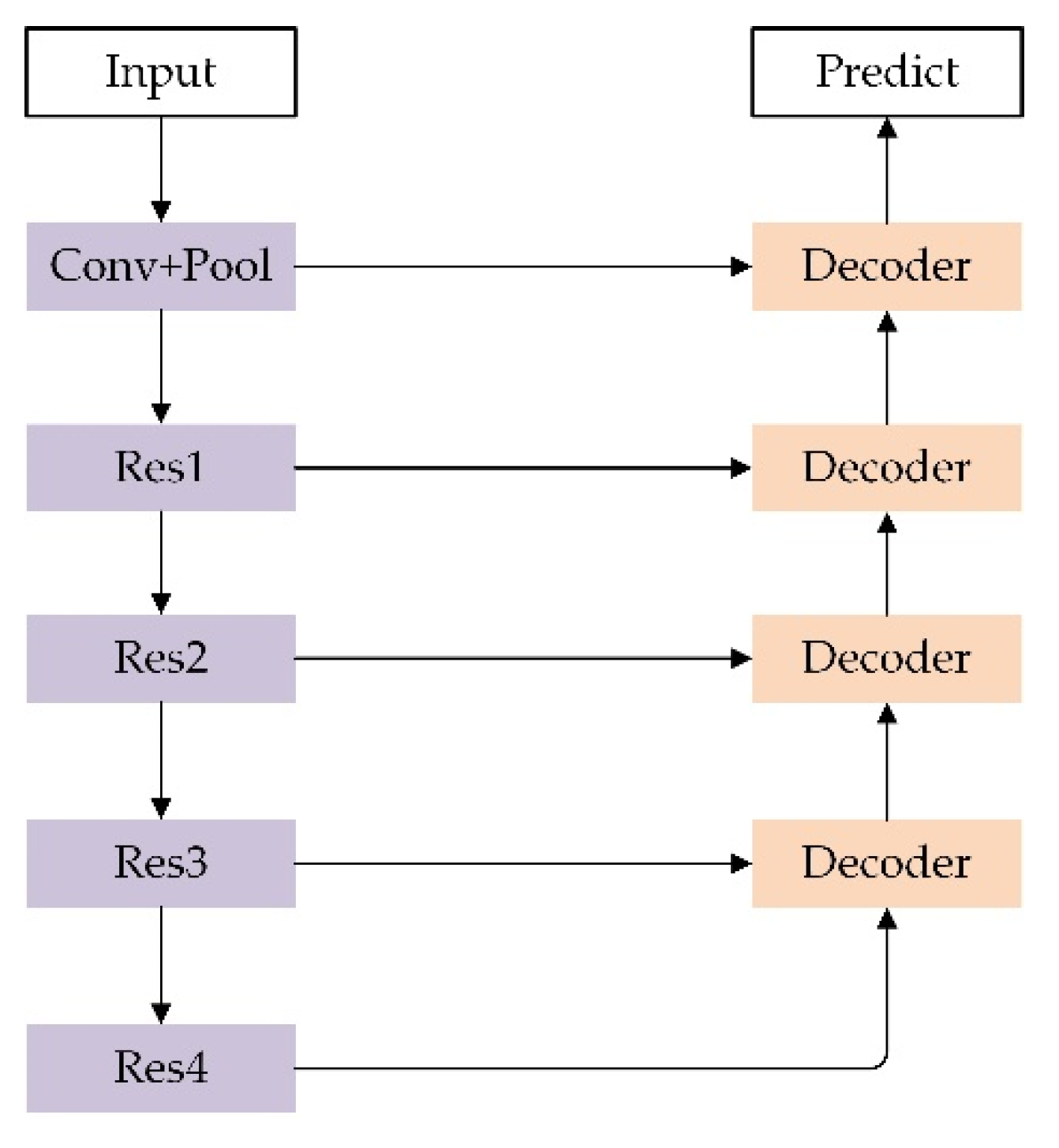
U-Net provides a concise symmetrical encoder–decoder structure. The encoder part consists of a series of convolution filters and max pooling operations. Symmetrically, a series of upsampling operations and convolution layers comprise the decoder part. In U-Net, high-level semantic features post-upsampling are concatenated with corresponding shallow-appearance features, and then they are merged via subsequent convolution layers. Thus, the detailed spatial information lost in the encoder part due to max pooling will gradually be recovered during the decoding process. Adequate integration of high-level semantic features and shallow-appearance features in U-Net facilitates the boundary extraction of targets and recognition of small objects. Figure 3 shows the U-Net architecture with ResNet as the backbone/encoder.

3.2. ResNet Backbone

To address the degradation problem when training deep networks, Kaiming et al. proposed a deep residual learning network [58]. Specifically, for a feature x, let the expected learned output via several stacked nonlinear layers be H(x). The residual network forces the stacked nonlinear layers to learn F(x) = H(x) − x by adding an identity mapping of x onto F(x). When x is H(x), the stacked nonlinear layers only need to learn a zero mapping F(x) = 0. If x is close to H(x), then it is also easier to learn a residual correction of x than to learn a new mapping from scratch. Residual learning provides easy optimization of deep residual networks [58]. Thus, we used ResNet as the backbone/encoder of our model in this study.
The architecture of U-Net with ResNet as the backbone is shown in Figure 3. An input image is filtered by Conv, Res1, Res2, Res3, and Res4, generating feature maps with sizes of 1/2, 1/4, 1/8, 1/16, and 1/32, the size of the input image. Conv represents the first convolution layer of ResNet. Res1, Res2, Res3, and Res4 represent the first, second, third, and fourth residual Conv block in ResNet, respectively. The high-level feature maps are gradually upsampled by 2× and merged with corresponding shallow feature maps in Decoder blocks. One decoder block contains two convolution blocks, which each consist of a 3 × 3 convolution layer, a batch normalization layer and a ReLU activation function. The feature map generated by the last Decoder block is passed through a 3 × 3 convolution layer, a 2× upsampling layer, and a sigmoid activation function to create the final prediction map.

3.3. ACFNet Architecture

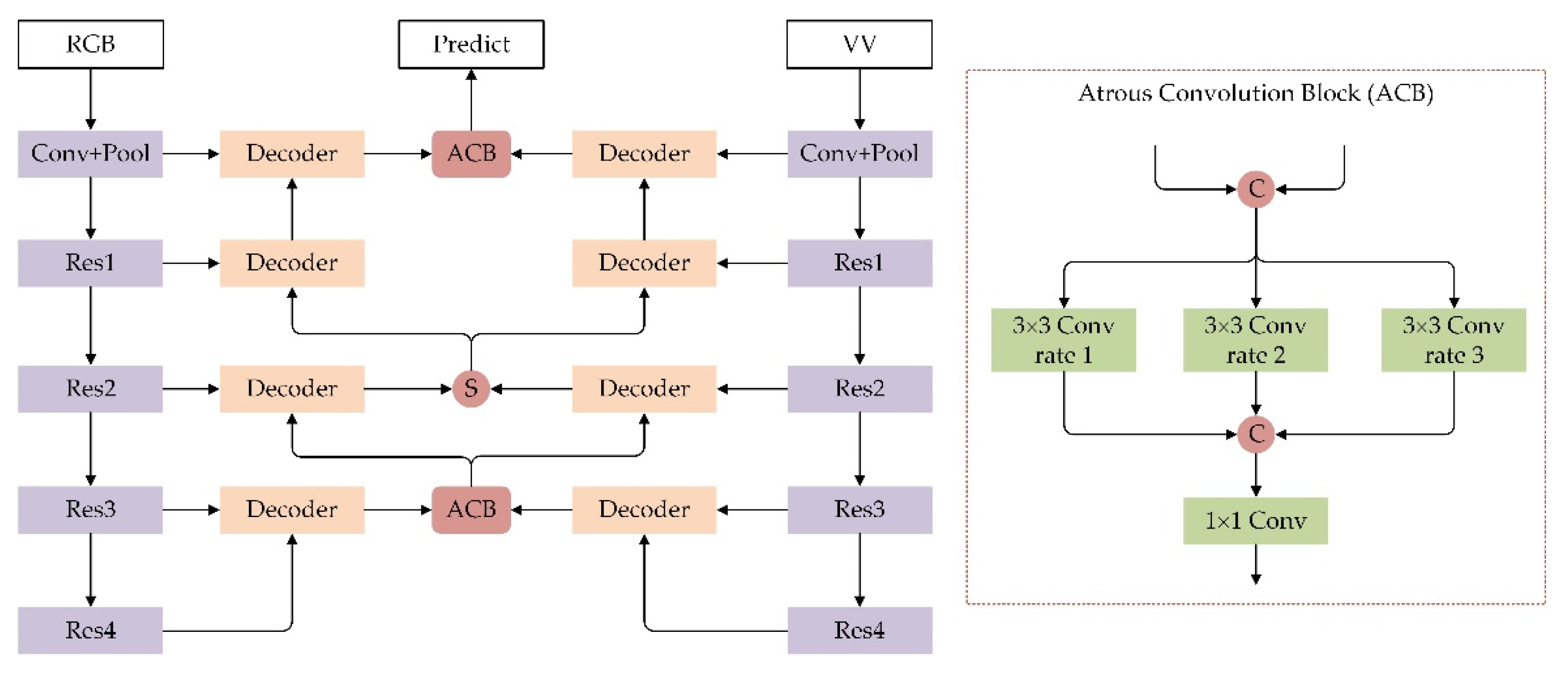
The architecture of the proposed ACFNet is shown in Figure 4. RGB and VV features are extracted by independent ResNet encoders. The first decoder block of each branch generates a group of features with a spatial size of 1/16, the size of the input image. The two groups of features are adequately fused through an atrous convolution block (ACB), as proposed. In this block, features of two modes are concatenated and filtered by three 3 × 3 atrous convolutions with dilated rates of 1, 2, and 3. Note that the 3 × 3 atrous convolution with a dilated rate of 1 is the standard 3 × 3 convolution. Atrous convolution allows for the fusion of two modes of features under a large receptive field while keeping the filter’s parameters constant. The three groups of features filtered under the different receptive fields are integrated by a 1 × 1 convolution. Note that the 1 × 1 convolution layer and 3 × 3 convolution layer in ACB are both followed by a batch normalization layer and a ReLU activation function. The integrated features flow parallelly into subsequent RGB and VV decoder branches to perform the second decoding separately. Features generated by the second decoder block of the RGB and VV branches are fused by an element-wise summation. The fused features continue to flow parallelly into subsequent RGB and VV decoder branches, and they pass through the last two Decoder blocks separately. The last Decoder block of each branch generates a group of features with more of this branch’s modality characteristics. To take full advantage of these two groups of semantic features for a highly accurate prediction, further integration is performed by an ACB again. Using the U-Net with ResNet as the backbone mentioned in Section 3.2, the last integrated semantic features are passed through a 3 × 3 convolution layer, a 2× upsampling layer, and a sigmoid activation function to generate the final prediction map.

3.4. Fusion Methods in the Encoder–Decoder Structure

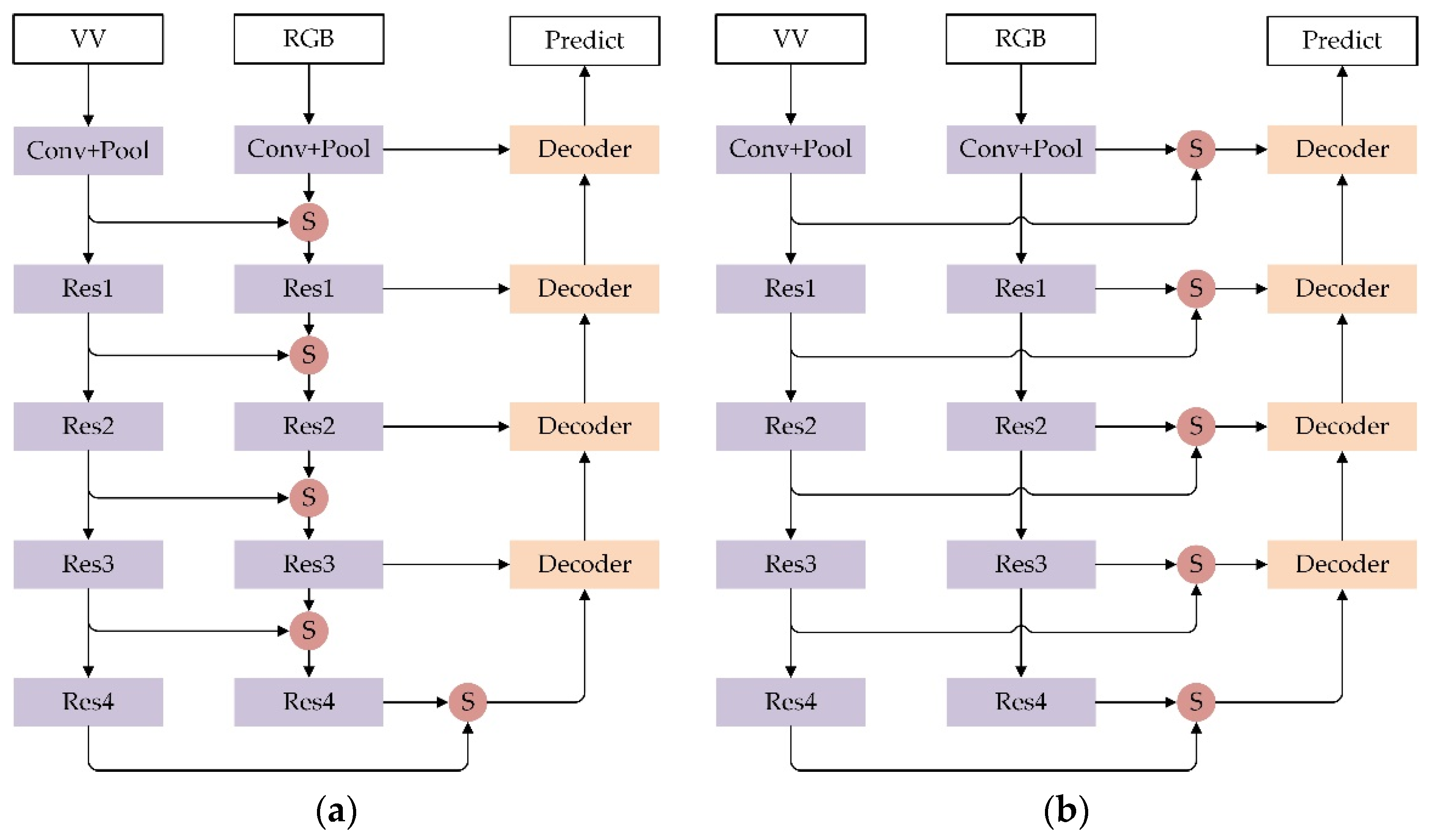
In the encoder–decoder semantic segmentation structure, the fusion of two modality data could occur at the input, encoder, decoder, or output, resulting in four fusion methods: (1) input fusion, in which two modality data are concatenated as the input data of a SS network [66]; (2) encoder fusion (Figure 5a), in which the extracted features of one modality data are always fused into corresponding extracted features of another modality data in the encoding process [67]; (3) decoder fusion (Figure 5b), in which the extracted features of two modality data in the encoding process are fused before they merge with high-level upsampled features in the decoding process [68,69,70]; and (4) output fusion, in which predictions made by two independent SS networks are fused by an element-wise summation to produce the final prediction. Regardless of the input fusion or output fusion, intermediate features are not fused. In this study, for a fair comparison of these four fusion methods in fusing RGB and VV data for glacial lake extraction, we adopted U-Net and ResNet as the structure and backbone/feature extractor, respectively, for the four fusion methods. The features are both fused via an element-wise summation in the encoder fusion and decoder fusion as shown in Figure 5. Comparing these four typical fusion models is helpful to explore the influence of the position where data fusion occurs on the networks’ performances.

4. Experiment and Results

4.1. Implementation Details

The implementation of our method is based on the PyTorch library. We used stochastic gradient descent (SGD) [71] to optimize the networks. The weight decay and momentum were set to 0.0001 and 0.9, respectively. We set the initial learning rate to 0.01. After 20 epochs, the learning rate decayed to 0.001 by multiplying by a factor of 0.1. The learning rate setting was found after a systematic search. The batch size was set to 16 due to the limited GPU memory, as in [62]. We trained all of the models for 50 epochs, which are enough for the models to converge.

4.2. Loss Function and Evaluation Metrics

In remote sensing images of the Himalayan regions, glacial lakes occupy a very small area compared with glaciers, vegetation, and bare land; thus, there is a large classification imbalance. In this situation, the widely used cross-entropy function for SS will bias network predictions towards background objects. To mitigate this issue, dice loss [72] was selected as our loss function to optimize the networks. The true positive (TP), false positive (FP), and false negative (FN) can be obtained by calculating the difference between the predictions and ground truth. According to the definition of dice coefficient in [73], the dice loss can be expressed as:
dice   loss = 1 2 TP 2 TP + FP + FN
Considering the large classification imbalance, we used precision, recall, F1, and intersection-over-union (IOU) [74] to evaluate the predictions of the networks on the test set. Precision is defined as:
precision = TP TP + FP
Precision, also known as user accuracy, reflects how many positive samples are correctly classified in the predictions. Recall is defined as:
recall = TP TP + FN
Recall, also known as producer accuracy, reflects how many positive samples in the ground truth are correctly predicted. F1 is defined as:
F 1 = 2 × precsion × recall precision + recall
The F1 score, a compromise between precision and recall, comprehensively reflects the prediction accuracy of a model. Note that the F1 score is actually the dice coefficient [73]. IOU can be expressed as:
IOU = TP TP + FP + FN
For binary classification, predictions and ground truth both belong to the set (0, 1). IOU is the ratio of the intersection of the two binary masks to the union of the two binary masks. A higher IOU correlates to a higher model prediction accuracy.

4.3. Results

Ref. [58] provided ResNets with various depths, which include 18-layer, 34-layer, 50-layer, 101-layer, and 152-layer ResNets. We trained and evaluated U-Nets with ResNets of different depths as the backbone. Given the limited GPU memory and time-consuming task of training very deep networks, 101-layer and 152-layer ResNets were not adopted in this study. The evaluation results of these U-Nets are detailed in Table 1. In addition to the four fusion methods and ACFNet mentioned in Section 3, we also trained and evaluated Wu’s model [46] and two other classical semantic segmentation models (SegNet and DeepLabV3+). Similar to ACFNet, Wu’s model was proposed to extract glacial lakes based on optical and SAR images. SegNet and DeepLabV3+ are advanced and popular in the semantic segmentation field. For a comparison with ACFNet, input fusion, Wu’s model, SegNet, and DeepLabV3+ all utilize 50-layer ResNet as the backbone. The evaluation results of input fusion, encoder fusion, decoder fusion, output fusion, SegNet, DeepLabV3+, Wu’s model, and ACFNet are detailed in Table 2.

5. Discussion

5.1. Backbone Depth for RGB and VV Data

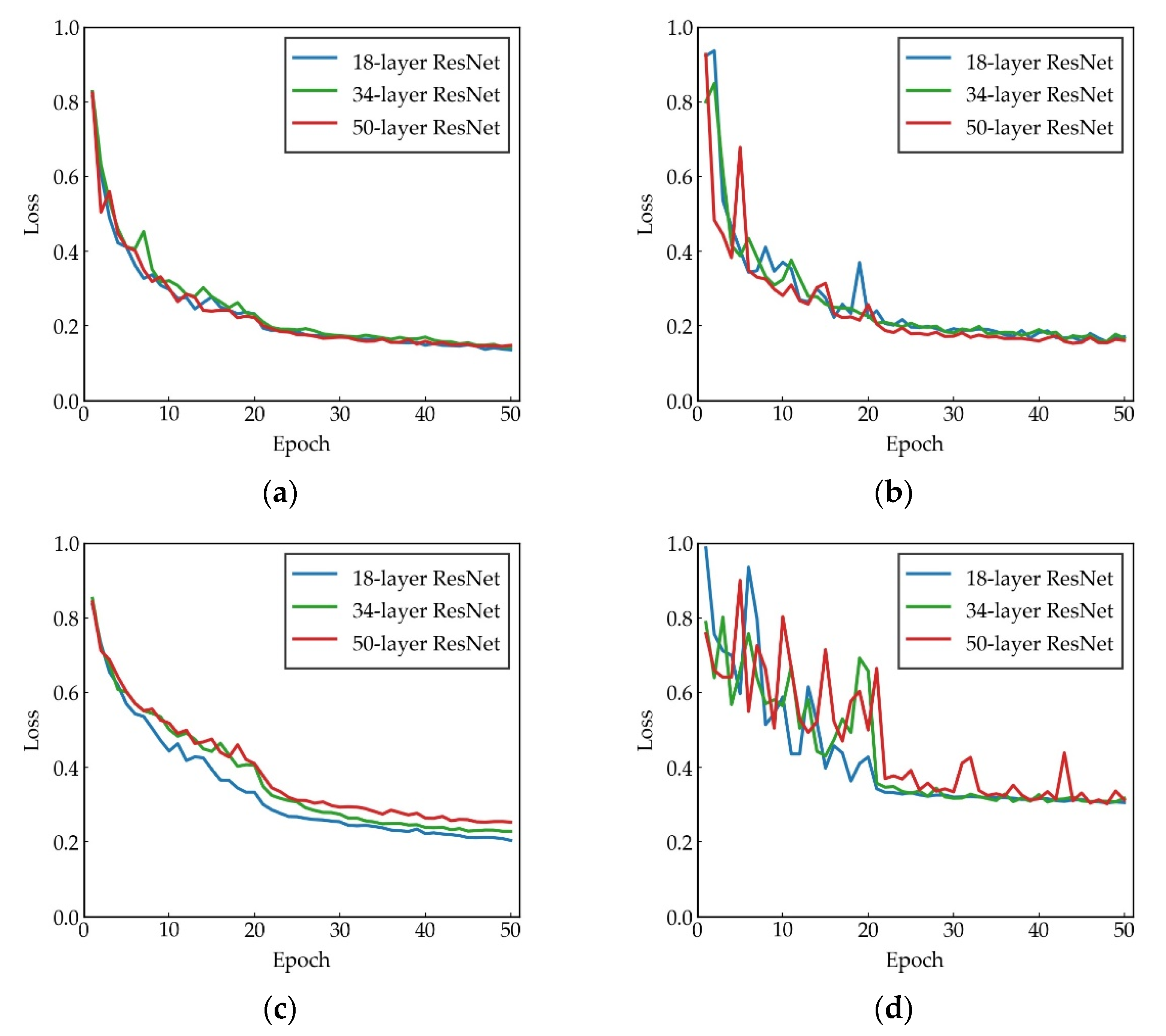
For the RGB data, as seen from Figure 6a, U-Nets with different depths present similar training curves. In the validation stage (Figure 6b), the U-Net with a 50-layer ResNet as the backbone produces a lower loss than the U-Nets with 18-layer and 34-layer ResNets as the backbone after 21 epochs.
For the test set, the U-Net with a 50-layer ResNet as the backbone achieved the highest IOU of 0.7724, as shown in Table 1. For the VV data, as seen in Figure 6c, the U-Net with an 18-layer ResNet as the backbone converged significantly faster than the U-Nets with 34-layer and 50-layer ResNets as the backbone, and it achieved the lowest training loss. In the validation (Figure 6d), the loss curves of the U-Nets with 18-layer and 34-layer ResNets as the backbone were more stable than the U-Net with a 50-layer ResNet as the backbone after 21 epochs. As shown in Table 1, the U-Net with an 18-layer ResNet as the backbone achieved the highest IOU of 0.5883 with the test set. Therefore, we chose 50-layer and 18-layer ResNets as the backbone/encoders of the RGB and VV branches, respectively, for ACFNet, encoder fusion, decoder fusion, and output fusion.

5.2. Effects of Fusion Methods

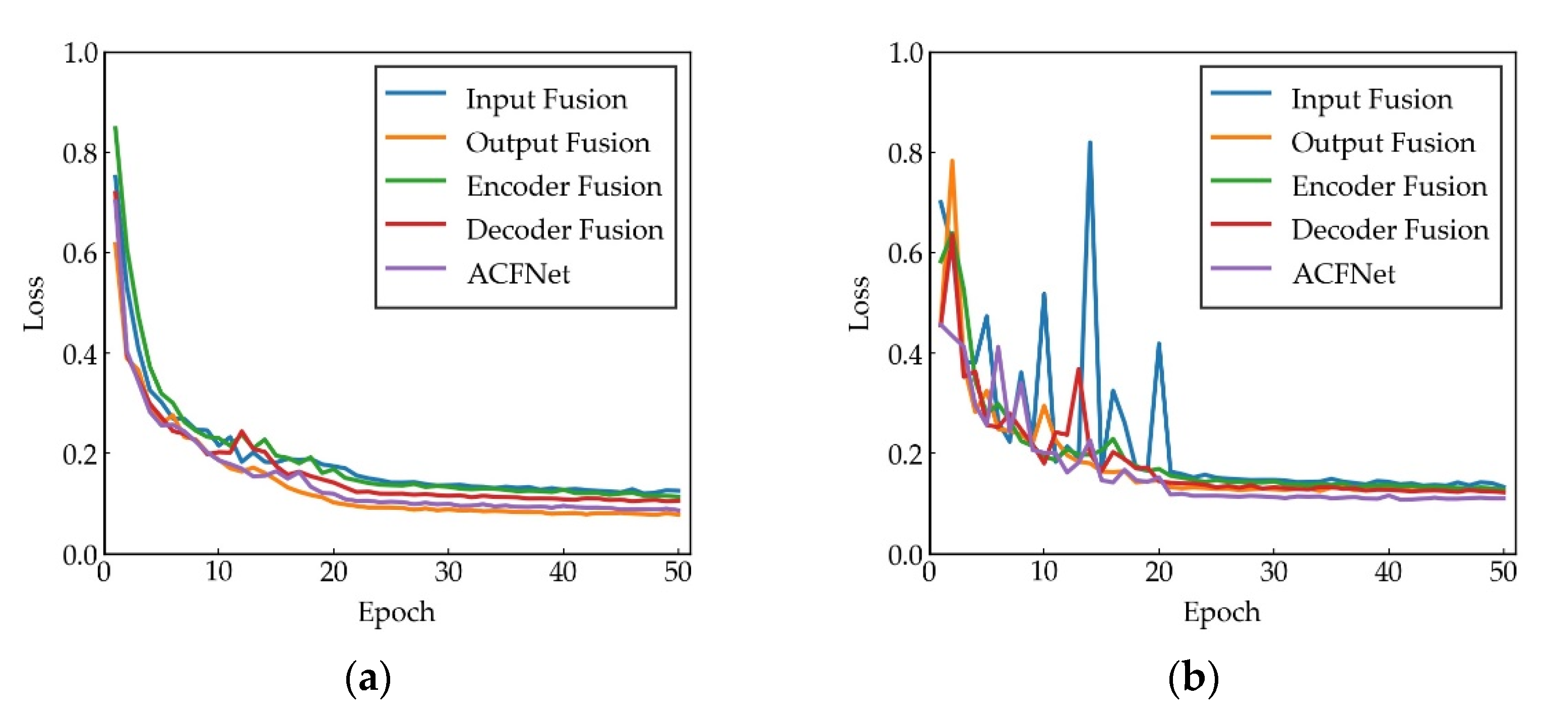
In this section, we discuss the effects of input fusion, encoder fusion, decoder fusion, output fusion, and ACFNet on fusing RGB and VV data for glacial lake extraction. Input fusion simply expands a RGB image’s channel with the addition of a SAR image’s VV band. RGB data reflect an object’s spectral information, while VV data reflect the geometrical structure of an object and its surroundings. Directly concatenating RGB and VV data as input is not appropriate because they are in two separate modalities but will go through the same network overall. Among the four fusion methods and our model, input fusion presented the highest loss during the training process and validation (Figure 7). As expected, input fusion also achieved a poor IOU of 0.7596 with the test set (Table 2). In addition, the imaging time of the VV images was close to that of the RGB images, but not the same, which signifies a difference in the texture of glacial lakes may exist between the two types of images. Therefore, the extracted objects’ texture features from RGB+VV images will be a mixture of an object’s texture features from RGB and VV images, bringing uncertainties to the network’s predictions.
Encoder fusion gradually incorporates the extracted VV features into the feature extraction branch of the RGB data via a summation method. In this process, VV and RGB features are fused at locations with different network depths. Due to the relatively sufficient feature fusion, encoder fusion achieved an IOU of 0.7944 with the test set (Table 2), which is 3.48% higher than that of input fusion. However, gradually integrating VV features with RGB features in the encoding process may have disturbed the feature extraction of the RGB data, because the features fed to the RGB branch’s encoding layers are a mixture of two modality features.
In decoder fusion, the feature extraction branches for the RGB and VV data at the encoder stage are independent, guaranteeing that the extracted features have their own modality characteristics. Note that decoder fusion has exactly the same number of parameters as encoder fusion. The only difference between decoder fusion and encoder fusion is that the extracted features are fused at different stages. However, decoder fusion converged faster than encoder fusion in the training process and presented lower loss during validation (Figure 7). With the test set, decoder fusion achieved an IOU of 0.8132 (Table 2), which is 1.88% higher than that of encoder fusion. This finding suggests that extracting RGB and VV features independently is better than incorporating VV features into RGB features during the encoding process.
Output fusion simply adds the prediction of the RGB branch to the prediction of the VV branch as the final prediction. No features of the RGB and VV data are fused in the encoding or decoding stage. Thus, there is no disturbance between the RGB and VV data in the encoding or decoding processes, facilitating the training of the network. Output fusion converged fastest in the training process and achieved the lowest training loss (Figure 7a). However, due to the poor predictive ability of the VV branch, output fusion performed worse than ACFNet in validation (Figure 7b). With the test set, output fusion achieved an IOU of 0.8067 (Table 2), which is 4.71% and 1.23% higher than that of input fusion and encoder fusion, respectively. This finding suggests that the sufficient extraction of characteristics of each modal data is vital for the full use of multimodal data. It is worth noting that output fusion achieved the highest precision of 0.9283 with the test set (Table 2). If the RGB branch and VV branch both believe a pixel is a glacial lake pixel, then this pixel has a high probability of being a glacial lake pixel. Because the prediction generated by output fusion can be regarded as the sum of probabilities given by RGB branch and VV branch.
Unlike the shallow features fused in encoder fusion and decoder fusion, the features generated by the first and the second decoder blocks in ACFNet are at deep positions in the network. Thus, these features have a higher level of semantic information than the shallow features with the same spatial size. Fusing two modality features with high-level semantics could mitigate the negative influence caused by the different imaging times of optical and SAR images. ACFNet is improved based on output fusion. In output fusion, the two predictions of the RGB branch and VV branch are simply fused by an element-wise summation. There are no neurons to learn the relationship between these two predictions. In ACFNet, two groups of features generated by the last decoder block of the RGB branch and VV branch are fused through the atrous convolution block. In this block, many neurons learn a nonlinear map to convert these two groups of features to a new group of features for a prediction with high accuracy. Because of the two additional atrous convolution blocks, ACFNet is not easy to train compared with output fusion and achieves higher training loss than output fusion (Figure 7a). However, ACFNet achieved the lowest loss in validation (Figure 7b) and the highest IOU of 0.8278 with the test set (Table 2), which is 2.11% higher than that of output fusion. This indicates that our network architecture and atrous convolution block are effective for fusing RGB and VV data for glacial lake extraction.

5.3. Comparisons with Other Models

As shown in Table 2, Wu’s model achieves a higher IOU than input fusion, with a margin of 2.65%; this indicates that concatenating the shallow features of the RGB and VV images as an input is better than directly concatenating the RGB and VV images as an input. Because Wu’s model cannot effectively extract and blend features of the RGB and VV data, its IOU was lower than that of ACFNet, with a large margin of 4.17%. Although SegNet utilizes max pooling indices stored in the encoding process to recover details in the decoding process, it achieved the worst IOU of 0.7221 with the test set (Table 2), which is 3.75% lower than that of input fusion. This result indicates that shallow features could provide more information than max pooling indices for recovering object details. DeepLabV3+ achieved an IOU of 0.7389, which is 2.07% lower than that of input fusion, because 4X upsampling at the end of the network caused the prediction loss of many boundary details of glacial lakes. Like input fusion, SegNet and DeepLabV3+ simply concatenate the RGB and VV images as input without specifically extracting and blending two modality features. Thus, their performances with the test set were far inferior to ACFNet (Table 2). Figure 8 shows the glacial lake extraction effects of input fusion, encoder fusion, decoder fusion, output fusion, ACFNet, Wu’s model, SegNet, and DeepLabV3+.

5.4. Impacts of Imaging Time Intervals between SAR and Optical Images

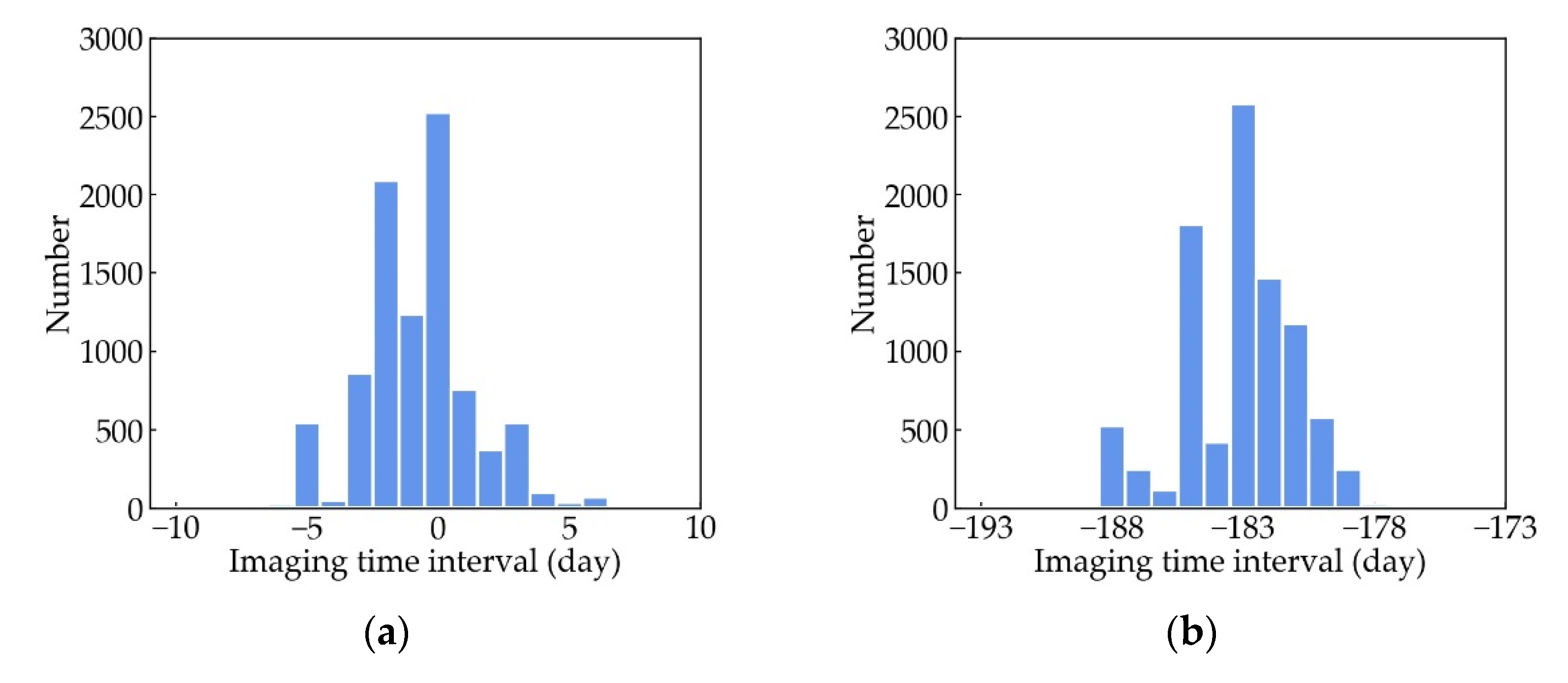
In our dataset, the imaging time of each SAR patch was as close to the corresponding optical patch as possible. The distribution of the imaging time intervals between the SAR patches and optical patches is shown in Figure 9a. Approximately 95.56% of the imaging time intervals were within six days. Thus, the edge details of the glacial lakes in the SAR images are very similar to those in the optical images. Given that our optical images were mainly acquired during autumn when seasonal snowfall is sparse, the glacial lakes in the SAR images exhibit a flat interior and a low backscatter coefficient, as shown in the “good” VV column of Figure 2b. Short imaging time intervals between the SAR and optical images are vital to the success of multisource data fusion. To further understand the impacts of the imaging time intervals between the SAR and optical images for glacial lake extraction, we generated a set of SAR patches that were acquired half a year earlier than the optical patches. We call this set of SAR images the “bad” VV images. The distribution of the imaging time intervals between the “bad” VV patches and optical patches is shown in Figure 9b. Approximately 95.37% of the imaging time intervals were between −188 and −178 days. Thus, the “bad” VV images were mainly acquired between March and May. During this period, many glacial lakes have frozen surfaces or are partially covered by seasonal snowfall, resulting in a heterogeneous interior structure and a relatively high backscatter coefficient in the SAR images, as shown in the “bad” VV column of Figure 2b. This makes it difficult to distinguish glacial lakes from background objects in the “bad” VV images.
We trained and evaluated the models mentioned previously with the dataset comprising the RGB data and “bad” VV data. The evaluation results with the test set are detailed in Table 3. Compared with the evaluation results (Table 2) with the test set comprising the RGB data and “good” VV data, the accuracies of all of the models decreased. This is because the “bad” VV data cannot provide obvious features of glacial lakes due to the snow and ice covers. Wu’s model achieved the smallest IOU decrease of 0.54%. We attribute this result to the simple and inadequate fusion of the RGB features and VV features, which indicates that the model just needs to learn few parameters to ignore the “bad” VV features. When simply concatenating the RGB and VV images as input, input fusion produced a small IOU decrease of 0.63%. Similarly, DeepLabV3+ produced a small IOU decrease of 1.16%. The largest IOU decrease of 5.59% was achieved by SegNet. Although the RGB and VV images were simply concatenated as input in SegNet, “bad” VV data produced incorrect max pooling indices that influenced the network’s decoding process and predictions. Output fusion also produced a large IOU decrease of 4.22% due to the poor predictions of the “bad” VV data. Encoder fusion, decoder fusion, and ACFNet achieved relatively large IOU decreases. We attribute this result to the sufficient feature fusion amplifying the effect of “bad” VV data. Even so, ACFNet achieved the highest IOU of 0.7814 among the eight methods (Table 3).

6. Conclusions

We proposed a feature fusion network (ACFNet) to extract glacial lakes using Landsat 8 optical RGB images and Sentinel-1 SAR VV images. In this proposed model, the features of optical images and SAR images were independently extracted by two CNN branches in the encoder stage. Two modality high-level semantic features generated by decoder blocks were adequately fused under different receptive fields by atrous convolution blocks. Input fusion, encoder fusion, decoder fusion, output fusion, SegNet, DeepLabV3+, and Wu’s model were compared with our model. Due to the sufficient feature extraction of single-modal data (optical/SAR) and the adequate fusion of optical and SAR features, our model achieved the best glacial lake extraction with an F1 score of 0.9057. Although the selected SAR patches had imaging times closest to those of the optical patches, the boundary details of the glacial lakes in these two types of images were slightly different. Fusing more advanced features that have a larger receptive field and more abstract semantics rather than shallow features will help to mitigate the influence of this discrepancy; this point also explains why our model works effectively. However, SAR images acquired in a different season than the optical images greatly affected those networks that adequately fuse optical and SAR features. This is because there are a lot of neurons needed to be suppressed to neglect the “bad” SAR features. Our method could be used to monitor the long-term changes of glacial lakes, providing a base for assessing risks of GLOFs and forecasting GLOFs. However, subject to the ubiquitous cloud and snow in the Himalaya and the revisit periods of the satellites, there would be many monitoring gaps. Note that SAR images are utilized as auxiliary data for optical data to extract glacial lakes in our method. If the glacial lakes are covered by cloud, our method would give uncertain predictions. Besides, the data used in this study were limited to optical RGB and SAR VV images. Given the complex environments in glaciated alpine regions, in future work, we will integrate additional data into the model, such as surface temperatures and DEM, to map glacial lakes with high accuracy.

Author Contributions

Conceptualization, J.W. and F.C.; methodology, J.W.; software, B.Y.; validation, M.Z. and B.Y.; formal analysis, J.W.; investigation, J.W.; resources, F.C.; data curation, M.Z.; writing—original draft preparation, J.W.; writing—review and editing, B.Y.; visualization, M.Z.; supervision, F.C.; project administration, M.Z.; funding acquisition, F.C. All authors have read and agreed to the published version of the manuscript.

Funding

This research was funded by the National Natural Science Foundation of China (41871345), and the Strategic Priority Research Program of the Chinese Academy of Sciences (XDA19030101).

Conflicts of Interest

The authors declare no conflict of interest.

References

  1. Zemp, M.; Huss, M.; Thibert, E.; Eckert, N.; McNabb, R.; Huber, J.; Barandun, M.; Machguth, H.; Nussbaumer, S.U.; Gartner-Roer, I.; et al. Global glacier mass changes and their contributions to sea-level rise from 1961 to 2016. Nature 2019, 568, 382–386. [Google Scholar] [CrossRef]
  2. Shugar, D.H.; Burr, A.; Haritashya, U.K.; Kargel, J.S.; Watson, C.S.; Kennedy, M.C.; Bevington, A.R.; Betts, R.A.; Harrison, S.; Strattman, K. Rapid worldwide growth of glacial lakes since 1990. Nat. Clim. Chang. 2020, 10, 939–945. [Google Scholar] [CrossRef]
  3. Wang, X.; Guo, X.; Yang, C.; Liu, Q.; Wei, J.; Zhang, Y.; Liu, S.; Zhang, Y.; Jiang, Z.; Tang, Z. Glacial lake inventory of high-mountain Asia in 1990 and 2018 derived from Landsat images. Earth Syst. Sci. Data 2020, 12, 2169–2182. [Google Scholar] [CrossRef]
  4. Chen, F.; Zhang, M.; Guo, H.; Allen, S.; Kargel, J.S.; Haritashya, U.K.; Watson, C.S. Annual 30 m dataset for glacial lakes in High Mountain Asia from 2008 to 2017. Earth Syst. Sci. Data 2021, 13, 741–766. [Google Scholar] [CrossRef]
  5. King, O.; Dehecq, A.; Quincey, D.; Carrivick, J. Contrasting geometric and dynamic evolution of lake and land-terminating glaciers in the central Himalaya. Glob. Planet. Chang. 2018, 167, 46–60. [Google Scholar] [CrossRef]
  6. Zheng, G.; Allen, S.K.; Bao, A.; Ballesteros-Cánovas, J.A.; Huss, M.; Zhang, G.; Li, J.; Yuan, Y.; Jiang, L.; Yu, T.; et al. Increasing risk of glacial lake outburst floods from future Third Pole deglaciation. Nat. Clim. Chang. 2021, 11, 411–417. [Google Scholar] [CrossRef]
  7. Dubey, S.; Goyal, M.K. Glacial Lake Outburst Flood Hazard, Downstream Impact, and Risk Over the Indian Himalayas. Water Resour. Res. 2020, 56, e2019WR026533. [Google Scholar] [CrossRef]
  8. Ashraf, A.; Naz, R.; Roohi, R. Glacial lake outburst flood hazards in Hindukush, Karakoram and Himalayan Ranges of Pakistan: Implications and risk analysis. Geomat. Nat. Hazards Risk 2012, 3, 113–132. [Google Scholar] [CrossRef] [Green Version]
  9. Khanal, N.R.; Mool, P.K.; Shrestha, A.B.; Rasul, G.; Ghimire, P.K.; Shrestha, R.B.; Joshi, S.P. A comprehensive approach and methods for glacial lake outburst flood risk assessment, with examples from Nepal and the transboundary area. Int. J. Water Resour. Dev. 2015, 31, 219–237. [Google Scholar] [CrossRef] [Green Version]
  10. Petrov, M.A.; Sabitov, T.Y.; Tomashevskaya, I.G.; Glazirin, G.E.; Chernomorets, S.S.; Savernyuk, E.A.; Tutubalina, O.V.; Petrakov, D.A.; Sokolov, L.S.; Dokukin, M.D.; et al. Glacial lake inventory and lake outburst potential in Uzbekistan. Sci. Total Environ. 2017, 592, 228–242. [Google Scholar] [CrossRef] [PubMed] [Green Version]
  11. Prakash, C.; Nagarajan, R. Glacial lake changes and outburst flood hazard in Chandra basin, North-Western Indian Himalaya. Geomat. Nat. Hazards Risk 2018, 9, 337–355. [Google Scholar] [CrossRef] [Green Version]
  12. Brun, F.; Wagnon, P.; Berthier, E.; Jomelli, V.; Maharjan, S.B.; Shrestha, F.; Kraaijenbrink, P.D.A. Heterogeneous Influence of Glacier Morphology on the Mass Balance Variability in High Mountain Asia. J. Geophys. Res. Earth Surf. 2019, 124, 1331–1345. [Google Scholar] [CrossRef]
  13. King, O.; Bhattacharya, A.; Bhambri, R.; Bolch, T. Glacial lakes exacerbate Himalayan glacier mass loss. Sci. Rep. 2019, 9, 18145. [Google Scholar] [CrossRef] [Green Version]
  14. Carrivick, J.L.; Tweed, F.S. Proglacial lakes: Character, behaviour and geological importance. Quat. Sci. Rev. 2013, 78, 34–52. [Google Scholar] [CrossRef] [Green Version]
  15. Ukita, J.; Narama, C.; Tadono, T.; Yamanokuchi, T.; Tomiyama, N.; Kawamoto, S.; Abe, C.; Uda, T.; Yabuki, H.; Fujita, K. Glacial lake inventory of Bhutan using ALOS data: Methods and preliminary results. Ann. Glaciol. 2011, 52, 65–71. [Google Scholar] [CrossRef] [Green Version]
  16. Wang, X.; Siegert, F.; Zhou, A.-g.; Franke, J. Glacier and glacial lake changes and their relationship in the context of climate change, Central Tibetan Plateau 1972–2010. Glob. Planet. Chang. 2013, 111, 246–257. [Google Scholar] [CrossRef]
  17. Wang, W.; Xiang, Y.; Gao, Y.; Lu, A.; Yao, T. Rapid expansion of glacial lakes caused by climate and glacier retreat in the Central Himalayas. Hydrol. Process. 2015, 29, 859–874. [Google Scholar] [CrossRef]
  18. Zhang, G.; Yao, T.; Xie, H.; Wang, W.; Yang, W. An inventory of glacial lakes in the Third Pole region and their changes in response to global warming. Glob. Planet. Chang. 2015, 131, 148–157. [Google Scholar] [CrossRef]
  19. Raj, K.B.G.; Kumar, K.V. Inventory of Glacial Lakes and its Evolution in Uttarakhand Himalaya Using Time Series Satellite Data. J. Indian Soc. Remote Sens. 2016, 44, 959–976. [Google Scholar] [CrossRef]
  20. Senese, A.; Maragno, D.; Fugazza, D.; Soncini, A.; D’Agata, C.; Azzoni, R.S.; Minora, U.; Ul-Hassan, R.; Vuillermoz, E.; Asif Khan, M.; et al. Inventory of glaciers and glacial lakes of the Central Karakoram National Park (CKNP–Pakistan). J. Maps 2018, 14, 189–198. [Google Scholar] [CrossRef]
  21. McFeeters, S.K. The use of the Normalized Difference Water Index (NDWI) in the delineation of open water features. Int. J. Remote Sens. 1996, 17, 1425–1432. [Google Scholar] [CrossRef]
  22. Worni, R.; Huggel, C.; Stoffel, M. Glacial lakes in the Indian Himalayas--from an area-wide glacial lake inventory to on-site and modeling based risk assessment of critical glacial lakes. Sci. Total Environ. 2013, 468–469, S71–S84. [Google Scholar] [CrossRef] [PubMed]
  23. Xin, W.; Shiyin, L.; Wanqin, G.; Xiaojun, Y.; Zongli, J.; Yongshun, H. Using Remote Sensing Data to Quantify Changes in Glacial Lakes in the Chinese Himalaya. Mt. Res. Dev. 2012, 32, 203–212. [Google Scholar] [CrossRef]
  24. Huggel, C.; Kääb, A.; Haeberli, W.; Teysseire, P.; Paul, F. Remote sensing based assessment of hazards from glacier lake outbursts: A case study in the Swiss Alps. Can. Geotech. J. 2002, 39, 316–330. [Google Scholar] [CrossRef] [Green Version]
  25. Bolch, T.; Buchroithner, M.F.; Peters, J.; Baessler, M.; Bajracharya, S. Identification of glacier motion and potentially dangerous glacial lakes in the Mt. Everest region/Nepal using spaceborne imagery. Nat. Hazards Earth Syst. Sci. 2008, 8, 1329–1340. [Google Scholar] [CrossRef] [Green Version]
  26. Wang, X.; Liu, Q.; Liu, S.; Wei, J.; Jiang, Z. Heterogeneity of glacial lake expansion and its contrasting signals with climate change in Tarim Basin, Central Asia. Environ. Earth Sci. 2016, 75, 696. [Google Scholar] [CrossRef]
  27. Wang, X.I.N.; Chai, K.; Liu, S.; Wei, J.; Jiang, Z.; Liu, Q. Changes of glaciers and glacial lakes implying corridor-barrier effects and climate change in the Hengduan Shan, southeastern Tibetan Plateau. J. Glaciol. 2017, 63, 535–542. [Google Scholar] [CrossRef] [Green Version]
  28. Shukla, A.; Garg, P.K.; Srivastava, S. Evolution of Glacial and High-Altitude Lakes in the Sikkim, Eastern Himalaya Over the Past Four Decades (1975–2017). Front. Environ. Sci. 2018, 6, 81. [Google Scholar] [CrossRef]
  29. Gardelle, J.; Arnaud, Y.; Berthier, E. Contrasted evolution of glacial lakes along the Hindu Kush Himalaya mountain range between 1990 and 2009. Glob. Planet. Chang. 2011, 75, 47–55. [Google Scholar] [CrossRef] [Green Version]
  30. Bhardwaj, A.; Singh, M.K.; Joshi, P.K.; Snehmani; Singh, S.; Sam, L.; Gupta, R.D.; Kumar, R. A lake detection algorithm (LDA) using Landsat 8 data: A comparative approach in glacial environment. Int. J. Appl. Earth Obs. Geoinf. 2015, 38, 150–163. [Google Scholar] [CrossRef]
  31. Li, J.; Sheng, Y.; Luo, J. Automatic extraction of Himalayan glacial lakes with remote sensing. Yaogan Xuebao-J. Remote Sens. 2011, 15, 29–43. [Google Scholar]
  32. Song, C.; Sheng, Y.; Ke, L.; Nie, Y.; Wang, J. Glacial lake evolution in the southeastern Tibetan Plateau and the cause of rapid expansion of proglacial lakes linked to glacial-hydrogeomorphic processes. J. Hydrol. 2016, 540, 504–514. [Google Scholar] [CrossRef] [Green Version]
  33. Chen, F.; Zhang, M.; Tian, B.; Li, Z. Extraction of Glacial Lake Outlines in Tibet Plateau Using Landsat 8 Imagery and Google Earth Engine. IEEE J. Sel. Top. Appl. Earth Obs. Remote Sens. 2017, 10, 4002–4009. [Google Scholar] [CrossRef]
  34. Zhao, H.; Chen, F.; Zhang, M. A Systematic Extraction Approach for Mapping Glacial Lakes in High Mountain Regions of Asia. IEEE J. Sel. Top. Appl. Earth Obs. Remote Sens. 2018, 11, 2788–2799. [Google Scholar] [CrossRef]
  35. Jain, S.K.; Sinha, R.K.; Chaudhary, A.; Shukla, S. Expansion of a glacial lake, Tsho Chubda, Chamkhar Chu Basin, Hindukush Himalaya, Bhutan. Nat. Hazards 2014, 75, 1451–1464. [Google Scholar] [CrossRef]
  36. Veh, G.; Korup, O.; Roessner, S.; Walz, A. Detecting Himalayan glacial lake outburst floods from Landsat time series. Remote Sens. Environ. 2018, 207, 84–97. [Google Scholar] [CrossRef]
  37. Ma, L.; Liu, Y.; Zhang, X.; Ye, Y.; Yin, G.; Johnson, B.A. Deep learning in remote sensing applications: A meta-analysis and review. ISPRS J. Photogramm. Remote Sens. 2019, 152, 166–177. [Google Scholar] [CrossRef]
  38. Yu, B.; Chen, F.; Xu, C. Landslide detection based on contour-based deep learning framework in case of national scale of Nepal in 2015. Comput. Geosci. 2020, 135, 104388. [Google Scholar] [CrossRef]
  39. Yu, B.; Yang, L.; Chen, F. Semantic segmentation for high spatial resolution remote sensing images based on convolution neural network and pyramid pooling module. IEEE J. Sel. Top. Appl. Earth Obs. Remote Sens. 2018, 11, 3252–3261. [Google Scholar] [CrossRef]
  40. Chen, Y.; Li, L.; Whiting, M.; Chen, F.; Sun, Z.; Song, K.; Wang, Q. Convolutional neural network model for soil moisture prediction and its transferability analysis based on laboratory Vis-NIR spectral data. Int. J. Appl. Earth Obs. Geoinf. 2021, 104, 102550. [Google Scholar] [CrossRef]
  41. Guo, H.; Chen, F.; Sun, Z.; Liu, J.; Liang, D. Big Earth Data: A practice of sustainability science to achieve the Sustainable Development Goals. Sci. Bull. 2021, 66, 1050–1053. [Google Scholar] [CrossRef]
  42. Shamshirband, S.; Rabczuk, T.; Chau, K.-W. A survey of deep learning techniques: Application in wind and solar energy resources. IEEE Access 2019, 7, 164650–164666. [Google Scholar] [CrossRef]
  43. Fan, Y.; Xu, K.; Wu, H.; Zheng, Y.; Tao, B. Spatiotemporal modeling for nonlinear distributed thermal processes based on KL decomposition, MLP and LSTM network. IEEE Access 2020, 8, 25111–25121. [Google Scholar] [CrossRef]
  44. Qayyum, N.; Ghuffar, S.; Ahmad, H.; Yousaf, A.; Shahid, I. Glacial Lakes Mapping Using Multi Satellite PlanetScope Imagery and Deep Learning. ISPRS Int. J. Geo-Inf. 2020, 9, 560. [Google Scholar] [CrossRef]
  45. Chen, F. Comparing Methods for Segmenting Supra-Glacial Lakes and Surface Features in the Mount Everest Region of the Himalayas Using Chinese GaoFen-3 SAR Images. Remote Sens. 2021, 13, 2429. [Google Scholar] [CrossRef]
  46. Wu, R.; Liu, G.; Zhang, R.; Wang, X.; Li, Y.; Zhang, B.; Cai, J.; Xiang, W. A Deep Learning Method for Mapping Glacial Lakes from the Combined Use of Synthetic-Aperture Radar and Optical Satellite Images. Remote Sens. 2020, 12, 4020. [Google Scholar] [CrossRef]
  47. Badrinarayanan, V.; Kendall, A.; Cipolla, R. SegNet: A Deep Convolutional Encoder-Decoder Architecture for Image Segmentation. IEEE Trans. Pattern Anal. Mach. Intell. 2017, 39, 2481–2495. [Google Scholar] [CrossRef] [PubMed]
  48. Chen, L.-C.; Zhu, Y.; Papandreou, G.; Schroff, F.; Adam, H. Encoder-decoder with atrous separable convolution for semantic image segmentation. In Proceedings of the European conference on computer vision (ECCV), Munich, Germany, 8–14 September 2018; pp. 801–818. [Google Scholar]
  49. Song, C.; Sheng, Y.; Wang, J.; Ke, L.; Madson, A.; Nie, Y. Heterogeneous glacial lake changes and links of lake expansions to the rapid thinning of adjacent glacier termini in the Himalayas. Geomorphology 2017, 280, 30–38. [Google Scholar] [CrossRef] [Green Version]
  50. Bolch, T.; Kulkarni, A.; Kääb, A.; Huggel, C.; Paul, F.; Cogley, J.G.; Frey, H.; Kargel, J.S.; Fujita, K.; Scheel, M. The state and fate of Himalayan glaciers. Science 2012, 336, 310–314. [Google Scholar] [CrossRef] [Green Version]
  51. Brun, F.; Berthier, E.; Wagnon, P.; Kaab, A.; Treichler, D. A spatially resolved estimate of High Mountain Asia glacier mass balances, 2000–2016. Nat. Geosci. 2017, 10, 668–673. [Google Scholar] [CrossRef] [PubMed]
  52. Bookhagen, B.; Burbank, D.W. Toward a complete Himalayan hydrological budget: Spatiotemporal distribution of snowmelt and rainfall and their impact on river discharge. J. Geophys. Res. 2010, 115. [Google Scholar] [CrossRef] [Green Version]
  53. Nie, Y.; Sheng, Y.; Liu, Q.; Liu, L.; Liu, S.; Zhang, Y.; Song, C. A regional-scale assessment of Himalayan glacial lake changes using satellite observations from 1990 to 2015. Remote Sens. Environ. 2017, 189, 1–13. [Google Scholar] [CrossRef] [Green Version]
  54. Chen, F.; Yu, B.; Li, B. A practical trial of landslide detection from single-temporal Landsat8 images using contour-based proposals and random forest: A case study of national Nepal. Landslides 2018, 15, 453–464. [Google Scholar] [CrossRef]
  55. Wang, N.; Chen, F.; Yu, B.; Qin, Y. Segmentation of large-scale remotely sensed images on a Spark platform: A strategy for handling massive image tiles with the MapReduce model. ISPRS J. Photogramm. Remote Sens. 2020, 162, 137–147. [Google Scholar] [CrossRef]
  56. Schmitt, M.; Hughes, L.H.; Zhu, X.X. The SEN1-2 dataset for deep learning in SAR-optical data fusion. arXiv 2018, arXiv:1807.01569. [Google Scholar] [CrossRef] [Green Version]
  57. Versaci, M.; Calcagno, S.; Morabito, F.C. Fuzzy geometrical approach based on unit hyper-cubes for image contrast enhancement. In Proceedings of the 2015 IEEE International Conference on Signal and Image Processing Applications (ICSIPA), Kuala Lumpur, Malaysia, 19–21 October 2015; pp. 488–493. [Google Scholar]
  58. He, K.; Zhang, X.; Ren, S.; Sun, J. Deep residual learning for image recognition. In Proceedings of the IEEE conference on computer vision and pattern recognition, Las Vegas, NV, USA, 27–30 June 2016; pp. 770–778. [Google Scholar]
  59. Banan, A.; Nasiri, A.; Taheri-Garavand, A. Deep learning-based appearance features extraction for automated carp species identification. Aquac. Eng. 2020, 89, 102053. [Google Scholar] [CrossRef]
  60. Long, J.; Shelhamer, E.; Darrell, T. Fully convolutional networks for semantic segmentation. In Proceedings of the IEEE Conference on Computer Vision and Pattern Recognition, Boston, MA, USA, 7–12 June 2015; pp. 3431–3440. [Google Scholar]
  61. Ronneberger, O.; Fischer, P.; Brox, T. U-net: Convolutional networks for biomedical image segmentation. In Proceedings of the International Conference on Medical Image Computing and Computer-Assisted Intervention, Munich, Germany, 5–9 October 2015; pp. 234–241. [Google Scholar]
  62. Zhao, H.; Shi, J.; Qi, X.; Wang, X.; Jia, J. Pyramid scene parsing network. In Proceedings of the IEEE Conference on Computer vision and Pattern Recognition, Honolulu, HI, USA, 21–26 July 2017; pp. 2881–2890. [Google Scholar]
  63. Chen, L.-C.; Papandreou, G.; Kokkinos, I.; Murphy, K.; Yuille, A.L. Semantic image segmentation with deep convolutional nets and fully connected crfs. arXiv 2014, arXiv:1412.7062. [Google Scholar]
  64. Chen, L.-C.; Papandreou, G.; Kokkinos, I.; Murphy, K.; Yuille, A.L. Deeplab: Semantic image segmentation with deep convolutional nets, atrous convolution, and fully connected crfs. IEEE Trans. Pattern Anal. Mach. Intell. 2017, 40, 834–848. [Google Scholar] [CrossRef]
  65. Chen, L.-C.; Papandreou, G.; Schroff, F.; Adam, H. Rethinking atrous convolution for semantic image segmentation. arXiv 2017, arXiv:1706.05587. [Google Scholar]
  66. Couprie, C.; Farabet, C.; Najman, L.; LeCun, Y. Indoor semantic segmentation using depth information. arXiv 2013, arXiv:1301.3572. [Google Scholar]
  67. Hazirbas, C.; Ma, L.; Domokos, C.; Cremers, D. FuseNet: Incorporating depth into semantic segmentation via fusion-based CNN architecture. In Computer Vision–ACCV 2016; Lecture Notes in Computer Science; Springer: Berlin/Heidelberg, Germany, 2017; pp. 213–228. [Google Scholar]
  68. Ha, Q.; Watanabe, K.; Karasawa, T.; Ushiku, Y.; Harada, T. MFNet: Towards real-time semantic segmentation for autonomous vehicles with multi-spectral scenes. In Proceedings of the 2017 IEEE/RSJ International Conference on Intelligent Robots and Systems (IROS), Vancouver, BC, Canada, 24–28 September 2017; pp. 5108–5115. [Google Scholar]
  69. Adriano, B.; Yokoya, N.; Xia, J.; Miura, H.; Liu, W.; Matsuoka, M.; Koshimura, S. Learning from multimodal and multitemporal earth observation data for building damage mapping. ISPRS J. Photogramm. Remote. Sens. 2021, 175, 132–143. [Google Scholar] [CrossRef]
  70. Park, S.-J.; Hong, K.-S.; Lee, S. Rdfnet: Rgb-d multi-level residual feature fusion for indoor semantic segmentation. In Proceedings of the IEEE International Conference on Computer Vision, Venice, Italy, 22–29 October 2017; pp. 4980–4989. [Google Scholar]
  71. Bottou, L. Large-scale machine learning with stochastic gradient descent. In Proceedings of COMPSTAT’2010; Springer: Berlin/Heidelberg, Germany, 2010; pp. 177–186. [Google Scholar]
  72. Milletari, F.; Navab, N.; Ahmadi, S.-A. V-Net: Fully convolutional neural networks for volumetric medical image segmentation. In Proceedings of the 2016 Fourth International Conference on 3D Vision (3DV), Stanford, CA, USA, 25–28 October 2016; pp. 565–571. [Google Scholar]
  73. Li, X.; Sun, X.; Meng, Y.; Liang, J.; Wu, F.; Li, J. Dice loss for data-imbalanced NLP tasks. arXiv 2019, arXiv:1911.02855. [Google Scholar]
  74. Yu, B.; Chen, F.; Xu, C.; Wang, L.; Wang, N. Matrix SegNet: A Practical Deep Learning Framework for Landslide Mapping from Images of Different Areas with Different Spatial Resolutions. Remote Sens. 2021, 13, 3158. [Google Scholar] [CrossRef]
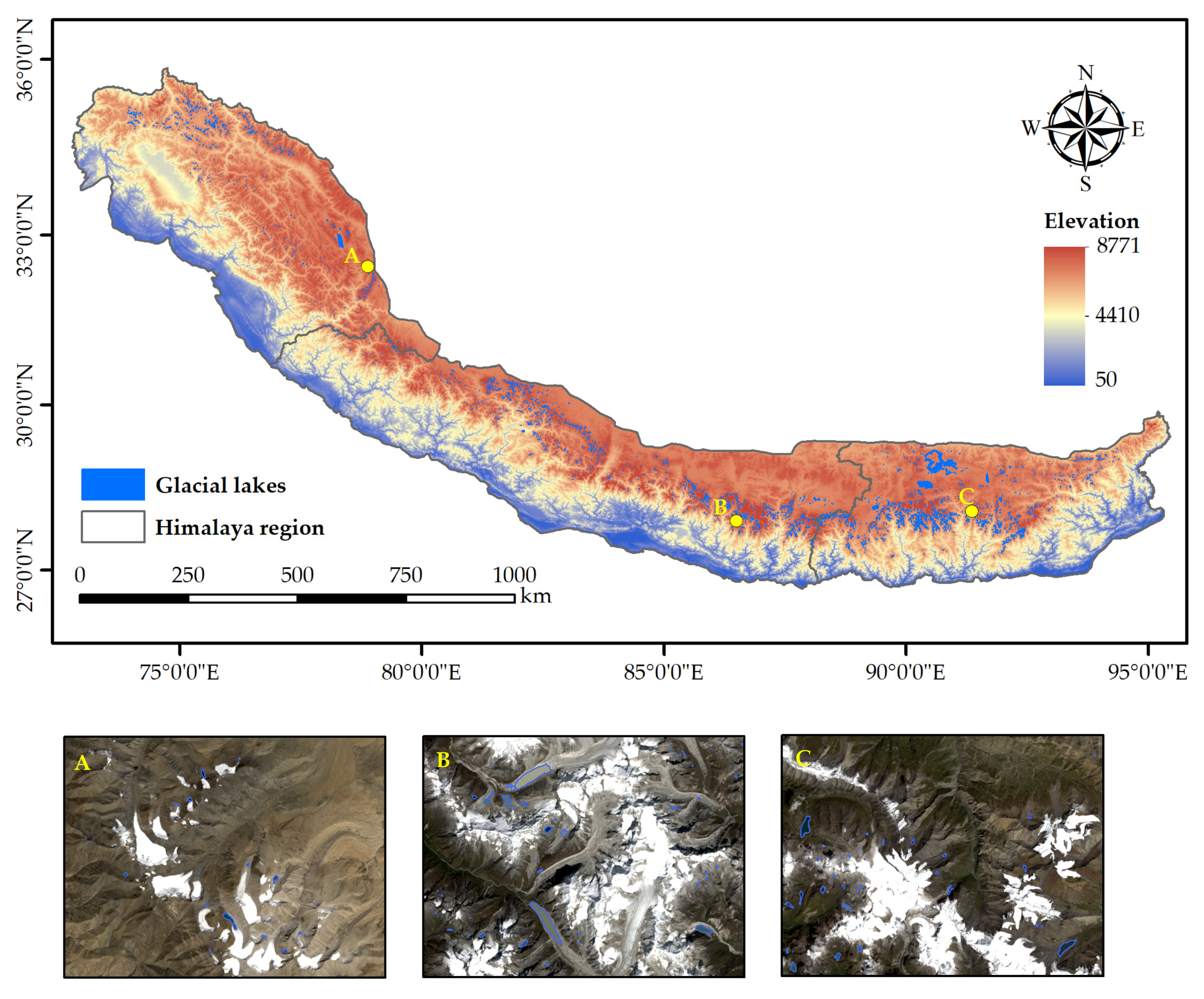
Figure 1. Distribution of glacial lakes in the Himalaya. The bottom row shows three local regions.
Remotesensing 13 05091 g001
Figure 2. (a) The flow diagram for preparing an optical-SAR patch pair; (b) RGB images and their corresponding “good” VV images with imaging times nearest those of the RGB images and “bad” VV images that were acquired half a year earlier than the RGB images.
Remotesensing 13 05091 g002
Figure 3. The architecture of U-Net with ResNet as the backbone.
Remotesensing 13 05091 g003
Figure 4. The architecture of ACFNet. ‘S’ represents an element-wise summation and ‘C’ represents a concatenation.
Remotesensing 13 05091 g004
Figure 5. (a) Encoder fusion; (b) decoder fusion. ‘S’ represents an element-wise summation.
Remotesensing 13 05091 g005
Figure 6. The training loss and validation loss of U-Nets with ResNets of various depths as the backbone for RGB data and VV data: (a) Training loss of RGB data; (b) validation loss of RGB data; (c) training loss of VV data; (d) validation loss of VV data.
Remotesensing 13 05091 g006
Figure 7. Training loss and validation loss of the five models: (a) Training loss; (b) validation loss.
Remotesensing 13 05091 g007
Figure 8. Glacial lake extraction effects of different methods. ‘GT’ represents ground truth. ‘F’ represents ‘Fusion’.
Remotesensing 13 05091 g008
Figure 9. Imaging time intervals between the SAR images and optical images: (a) Imaging time intervals between “good” VV patches and RGB patches; (b) imaging time intervals between “bad” VV patches and RGB patches.
Remotesensing 13 05091 g009
Table 1. The performance of U-Nets with ResNets of various depths as the backbone for the test set.
InputU-Net BackbonePrecisionRecallF1IOU
RGB18-layer ResNet0.92690.81390.86670.7649
34-layer ResNet0.91410.81740.8630.7591
50-layer ResNet0.91440.83260.87150.7724
VV18-layer ResNet0.810.68240.74070.5883
34-layer ResNet0.79270.68130.73280.5783
50-layer ResNet0.75820.69860.72720.5714
Table 2. The evaluation results of various methods for the test set.
InputModelPrecisionRecallF1IOU
RGB, VVWu’s Model0.8860.87450.88020.7861
ACFNet0.91980.89210.90570.8278
Output Fusion0.92830.86020.8930.8067
Decoder Fusion0.92150.87370.8970.8132
Encoder Fusion0.89460.87640.88540.7944
RGB+VVInput Fusion0.84760.87980.86340.7596
SegNet0.86250.8160.83860.7221
DeepLabV3+0.85570.84410.84980.7389
Table 3. The evaluation results of different methods with the test set comprising RGB data and “bad” VV data.
InputModelPrecisionRecallF1IOUIOU Decrease (%)
RGB, VVWu’s Model0.90830.84740.87680.78070.54
ACFNet0.90610.85020.87720.78144.64
Output Fusion0.9210.81810.86650.76454.22
Decoder Fusion0.91060.84360.87580.77913.41
Encoder Fusion0.88690.85160.86890.76822.62
RGB+VVInput Fusion0.8760.84320.85930.75330.63
SegNet0.84050.76260.79960.66625.59
DeepLabV3+0.88550.80280.84210.72731.16
Publisher’s Note: MDPI stays neutral with regard to jurisdictional claims in published maps and institutional affiliations.