Abstract
The spatial information about crop grain protein concentration (GPC) can be an important layer (i.e., a map that can be utilized in a geographic information system) with uses from nutrient management to grain marketing. Recently, on- and off-combine harvester sensors have been developed for creating spatial GPC layers. The quality of these GPC layers, as measured by the coefficient of determination (R2) and the root mean squared error (RMSE) of the relationship between measured and predicted GPC, is affected by different sensing characteristics. The objectives of this synthesis analysis were to (i) contrast GPC prediction R2 and RMSE for different sensor types (on-combine, off-combine proximal and remote); (ii) contrast and discuss the best spatial, temporal, and spectral resolutions and features, and the best statistical approach for off-combine sensors; and (iii) review current technology limitations and provide future directions for spatial GPC research and application. On-combine sensors were more accurate than remote sensors in predicting GPC, yet with similar precision. The most optimal conditions for creating reliable GPC predictions from off-combine sensors were sensing near anthesis using multiple spectral features that include the blue and green bands, and that are analyzed by complex statistical approaches. We discussed sensor choice in regard to previously identified uses of a GPC layer, and further proposed new uses with remote sensors including same season fertilizer management for increased GPC, and in advance segregated harvest planning related to field prioritization and farm infrastructure. Limitations of the GPC literature were identified and future directions for GPC research were proposed as (i) performing GPC predictive studies on a larger variety of crops and water regimes; (ii) reporting proper GPC ground-truth calibrations; (iii) conducting proper model training, validation, and testing; (iv) reporting model fit metrics that express greater concordance with the ideal predictive model; and (v) implementing and benchmarking one or more uses for a GPC layer.
1. Introduction
Grain protein concentration (GPC) is a critical trait, especially for crops with quality premium markets, such as wheat (Triticum aestivum L.). Commonly, producers harvest, store, and sell grain with potentially differing GPC but pricing at an average GPC level. Since GPC changes as a function of yield level [1,2,3,4,5], soil moisture [2,6,7], nitrogen (N) fertilizer [1,8,9], genotype, environment, and other management factors [6,7,8], even with similar yield levels a relatively uniform field is likely to produce spatially variable GPC and, if known, this information could be utilized by farmers for different purposes.
Knowing the magnitude and extent of spatial GPC variability can be used by farmers not only to segregate grain harvest for premium markets [9,10,11,12], but also as decision-making tools for nutrient management [13,14,15], and environmental compliance related to nutrient budgets (input minus removal) [16,17]. These three main uses of a spatial GPC layer have been discussed and summarized previously [18], considering the use of on-combine harvester GPC sensors. Since then, the literature of both on- and off-combine (i.e., ground and remote) sensing methods for creating a spatial GPC layer has expanded, with an increased interest in off-combine sensors. It is unclear how on- versus off-combine sensors compare when used to create a GPC layer, and a summary of the literature to assess their performance is lacking.
The three main methods used to create a spatial GPC layer are (i) hand sampling, (ii) on-combine proximal sensing; and (iii) off-combine proximal and remote sensing, which differ in complexity (i.e., the number of steps requiring expert knowledge to go from data collection to GPC layer) and scalability level. Hand sampling is the simplest and least scalable method, where grain samples are hand collected, georeferenced, analyzed in a laboratory for GPC, and then geostatistically interpolated to create a continuous spatial GPC layer [19].
On-combine proximal sensing utilizes sensors mounted in the combine, and it is scalable at field level. These sensors emit electromagnetic radiation, which interacts with grain samples during the harvest and records their spectral reflectance or transmittance at various wavelengths. The data is then related to GPC via calibration equations provided by the sensor manufacturer, which can be further fine tuned with field specific calibration. For further details about on-combine GPC sensors, see the review by [18].
Off-combine sensing options include, in order from least to most scalable: hand held [20,21]; ground based proximal sensors [22,23]; remote sensors mounted on unmanned [24,25] and manned [26,27] aerial vehicles; and satellite platform [28,29]. Most off-combine sensors measure light reflectance, are usually deployed in season, and use the plant canopy as the primary sensing target (i.e., an indirect measure of GPC potential) instead of the grain (i.e., a direct measure of GPC potential). As they are airborne and deployed during the growing season (in contrast to on-combine to at harvest sensing), off-combine sensing offers the advantages of (i) not requiring specialized combine sensing hardware at the farm level and, thus, being more cost-effective, (ii) allowing for same season GPC-based management, and (iii) in advance segregated harvest planning. However, these advantages may come at the expense of GPC prediction quality [28], and a formal quantitative summarized comparison to address this hypothesis is lacking in the literature.
Sensor measurements along with the observed GPC data and statistical modeling comprise the predictive system that creates a spatial GPC layer (i.e., a map that can be utilized in a geographic information system) at a given level of accuracy and precision. Typically, these two metrics are reported in the form of the coefficient of determination/R-squared (R2, larger is better) and root mean squared error (RMSE, smaller is better) of the relationship between the measured (benchmark dataset) and predicted GPC. Developments in sensors and statistical models have allowed for improvements in both R2 and RMSE in GPC prediction. For example, reported R2 values have increased from 0.31 to 0.98 [30] for on-combine, from 0.45 to 0.99 for off-combine proximal [31,32], and from 0.03 to 0.89 for off-combine remote sensors [33,34].
Despite the recent advancements, it is unclear how different sensor types (on-combine, off-combine proximal and remote) perform in predicting spatial GPC. For example, by sensing the grain directly as opposed to the canopy, GPC prediction by on-combine sensing is expected to outperform off-combine sensing, even though similar R2 and RMSE values have been reported for these types of sensing [14,35,36]. Furthermore, while on-combine sensors offer little to no control over sensing conditions, off-combine sensors offer a broad diversity of sensing/processing characteristics, such as different spatial, temporal, and spectral resolutions and features (bands and/or vegetation indices), and statistical modeling approaches. The scientific literature currently lacks a formal quantitative synthesis analysis of which off-combine sensing/processing characteristics are most likely to create reliable spatial GPC predictive models and identification of their potential limitations.
Therefore, the objectives of this study were to conduct a synthesis analysis of current/past scientific literature and summarize the findings related to (i) contrasting GPC prediction of the R2 and RMSE for different sensor types (on-combine, off-combine proximal and remote); (ii) contrasting and discussing, based on R2 and RMSE, the best spatial, temporal, and spectral resolutions and features, and the best statistical approach for off-combine sensors; and (iii) reviewing current technologies’ limitations and providing future directions for spatial GPC research and application.
2. Materials and Methods
A synthesis analysis of the literature has been conducted to collect and summarize studies reporting on the creation of a spatial GPC layer. The search was performed on the engines Google Scholar, Web of Science, and Web of Knowledge using the terms “on-combine”, “remote sensing”, “protein”, and “prediction”, last searched on November 2021 by two independent searchers. A study was included in the data base if it fulfilled the following search criteria: (i) it utilized one or more in field sensor types for GPC prediction, (ii) it collected ground truth GPC data, and (iii) it reported at least one of R2 or RMSE. Studies with the main text in a language other than English were not considered. Based on the title, abstract, and reference lists, a total of 202 studies were downloaded and further screened, and only 84 fulfilled all search criteria and were included in the final set. Each study received a unique entry (i.e., one table row) identification number (id). Studies reporting on more than one sensor and/or crop type were accommodated by allocating more than one data entry (i.e., one table row for each sensor and/or crop type for a given study, distinguished by different letters following the paper entry id). Therefore, a single publication could contribute more than one entry id to our main database. With that, the final data set was comprised of 105 entries across the 84 selected studies.
Selected papers were then summarized and had different variables extracted, including descriptors related to (i) study specific, and ii) sensor specific characteristics. Study specific characteristics included crop type, number of site years, ground truth GPC range (maximum–minimum observed GPC), and GPC sensor type (combine, proximal and remote). Sensor specific characteristics included GPC sensor spatial resolution (m), number of days sensed (grouped into classes 1, 2–5, 6–10 and >10 days), best sensing characteristics (timing, number of spectral features, type of spectral features, nonspectral covariables, spectral frequency), and best statistical approach (Table 1). Sensor specific characteristics did not apply to on-combine sensors and were collected only from off-combine studies.

Table 1.
Summary of the selected studies for the synthesis analysis. Entry identification, citation, study and sensor specific characteristics, and grain protein concentration model fit metrics. GPC = grain protein concentration, SS = single spectral, MS = multiple spectral, SD = single date, MD = multiple dates, Bivariatef = bivariate family, Multivariatef = multivariate family, PLSRf = partial least square regression family, RF-ANN = random forest artificial neural network, Max = maximum, Min = minimum, RMSE = root mean square error.
Best timing for sensing was extracted as either the single growth stage (for studies with one day sensed) or the growth stage with the greatest R2 (for studies with two or more days sensed) for GPC prediction. Best number of spectral features was characterized as whether a single spectral (only one band or vegetation index) or multiple spectral (more than one band and/or vegetation index) features were used in the greatest R2 model reported. Type of spectral feature is a binary response variable (i.e., yes/no) characterized as whether the best spectral feature (bands and/or vegetation indices) was comprised by the bands blue (400–500 nm), green (500–600 nm), red (600–700 nm), red-edge (700–800 nm), near-infrared (800–1300 nm), and short-wave infrared (1300–1900 nm).
Nonspectral covariables were characterized as whether the best number of spectral features included extra covariables (e.g., temperature, precipitation, gluten category, mechanistic crop modeling) and grouped into single spectral, single spectral + other, multiple spectral, multiple spectral + other. Best spectral frequency was characterized as whether spectral data from a single or multiple dates were used in the greatest R2 model reported in the study. Best statistical approach was characterized as whether the statistical analysis used in the greatest R2 model was part of the bivariate family (i.e., y~x), the multivariate family (i.e., y~x1 + x2 + … xn), the partial least-square regression (PLSR) family (including PLSR, powered PLSR and N-PLSR), or random forest artificial neural network (RF-ANN).
When available, both GPC model fit metrics of R2 and RMSE were extracted. In case a study reported multiple R2 and RMSE values (i.e., for different sites, years, crop growth stages, spectral features, and statistical model), the range of model fit metric values was extracted and summarized for each study. Studies reporting separate model fit metrics for different crops and/or sensor types had one model fit metric range for each combination among the studied and any of the crop and sensor types extracted.
The response variables maximum R2 and minimum RMSE were individually analyzed as a function of the explanatory variables sensor type, spatial resolution, number of days sensed, best timing, number of spectral features, type of spectral features, nonspectral covariables, spectral frequency, and statistical approach. Models were run as fixed effect analysis of variance (ANOVA) using the lm function from stats package [35]. Linear model assumptions of residual variance homogeneity and outlying residuals were checked using fitted vs. standardized residual plots, and residual normality was checked using quantile–quantile standardized residual plots. Model assumptions were deemed met and models were considered appropriate for inference. All statistical analyses were performed in R [35]. Computer code is available upon request.
3. Results
3.1. Search Summary, Building the Database
The majority of the studies were in wheat (69), followed by barley (Hordeum vulgare) (7), rice (Oryza sativa L.) (6), sorghum (Sorghum bicolor L.), maize (Zea mays), and soybeans (Glycine max) (2 each) (Table 1). The number of site years varied from 1 to 220, with a mean of 13 and median of 3. Minimum and maximum GPC were 5% and 20.1% for wheat, 6.7% and 16.6% for barley, 5.1% and 9.1% for rice, 5% and 15% for sorghum, 6.6% and 10.7% for maize, and 29% to 38.6% for soybeans (data not shown). The GPC range varied from 1.2% to 11%, with a mean of 5.6% and median of 5.8% (Table 1). The majority of the studies utilized proximal sensors (i.e., hand held and ground based sensors) (40), followed by remote sensors (i.e., sensors mounted on aerial vehicles and satellite platforms) (38), and combine (13) (Table 1).
For remote sensors, spatial resolution varied from 0.018 m to 1000 m with a mean of 64 m and median of 1.8 m. For remote and proximal sensors, the number of days sensed was grouped into the categories 1, 2–5, 6–10 and >10 days, with 39, 38, 4 and 10 entries in each category, respectively. A total of 13 different best timings for sensing were reported, whereby anthesis, heading, and grain filling were the most common (28, 13 and 8 entries, respectively, Supplementary Figure S1a). The best number of spectral features was single spectral in 60 entries and multiple spectral in 31 entries. The most frequent type of spectral features was, from most to least: NIR, red, green, red-edge, SWIR, and blue (Supplementary Table S1). The best spectral frequency was single date in 72 entries or multiple dates in 19 entries (Table 1). The best statistical approach was bivariate in 56 entries, multivariate in 12 entries, PLSR family in 18 entries, and RFF-ANN in 5 entries (Table 1).
Model fit metrics R2 and RMSE ranges were summarized and displayed as the maximum R2 and minimum RMSE reported for each combination among the studied and any of the crop and sensor types (Table 1). Model fit R2 was reported in 99 entries, ranging from 0.017 to 0.99, with a mean of 0.63 and median of 0.64. Of the 90 R2 entries, 76 were calculated on training data and 24 on validation data. Training data based R2 ranged from 0.02 to 0.99, with a mean of 0.6 and median of 0.61, and validation data based R2 ranged from 0.39 to 0.97, with a mean of 0.73 and median of 0.74. Model fit RMSE was reported in 55 entries, ranging from 0.016% to 1.65%, with a mean of 0.67% and median of 0.64%. Of the 55 RMSE entries, 20 were calculated on training data and 35 on validation data. Training data based RMSE ranged from 0.02% to 1.53%, with a mean of 0.70% and median of 0.64%, and validation data based RMSE ranged from 0.1% to 1.65%, with a mean of 0.66% and median of 0.57%.
3.2. Sensor Type
Both on- and off-combine (i.e., proximal and remote) sensor types were evaluated, with on-combine directly sensing the grain during harvest and off-combine sensing the crop canopy during the growing season. The overall distribution of the coefficient of determination (R2) and RMSE were obtained with the goal of synthesizing the knowledge on protein prediction for both on- and off-combine sensor types. Sensor type resulted in significant differences in maximum R2 (p = 0.005), with combine and proximal sensing having the greatest R2 (0.79 and 0.66 on average), and remote sensing the lowest R2 (0.57 on average) (Figure 1). The greatest maximum R2 reported for each sensor type was 0.98 (id = 40) for combine, 0.99 (ids = 63, 80) for proximal, and 0.93 (id = 76) for remote sensors (Table 1).

Figure 1.
Distribution of (a) maximum R2 and (b) minimum root mean squared error (RMSE) by sensor type (combine, proximal, remote). Black dot and lines represent the mean ± standard deviation, and n is the number of observations for each sensor type. In panel (a), means followed by the same letter are not significantly different at α = 0.05.
Sensor type resulted in similar minimum RMSE (p = 0.4), varying from 0.54% to 0.71% on average (Figure 1). The least minimum RMSE reported for each sensor type was 0.28% (id = 40) for combine, 0.02% (id = 63) for proximal, and 0.2% (id = 76) for remote sensors (Table 1). These proximal and remote sensor studies utilized multiple spectral features, single date sensing, and RF-ANN statistical analysis.
3.3. Spatial Resolution
Remote sensors’ spatial resolution ranged from 0.02 (id = 68) to 1000 m (ids 33, 36, 44, 52a) and resulted in similar maximum R2 (p = 0.64) and minimum RMSE (p = 0.99) (Supplementary Figure S1b,c). The spatial resolution observed in the study with greatest maximum R2 and least minimum RMSE (id = 76) was 0.02 m (Table 1).
3.4. Number of Days Sensed
The number of days sensed for proximal and remote sensors resulted in similar maximum R2 (p = 0.94) and minimum RMSE (p = 0.47) (Supplementary Figure S1d,e). The number of days sensed with the greatest maximum R2 for proximal sensors (ids = 63, 80) was 4 days (2–5 days category), and for remote sensors (id = 76) was 1 day. The number of days sensed with the least minimum RMSE for proximal sensors (id = 63) was 4 days (2–5 days category) and for remote sensors (id = 76) was 1 day (Table 1).
3.5. Number of Spectral Features
The number of spectral features for proximal and remote sensors used across study specific best models resulted in significant differences in maximum R2 (p = 0.02), with models that included multiple spectral features (more than one band and/or vegetation index) having greater maximum R2 (0.68 on average) than models including only a single spectral feature (0.57 on average) (Figure 2). The greatest maximum R2 observed for single spectral features was 0.99 (id = 80) and with multiple spectral features was 0.99 (id = 63) (Table 1). The number of spectral features resulted in similar minimum RMSE (p = 0.2), varying from 0.64% to 0.81% on average. The least minimum RMSE observed for single spectral features was 0.17% (id = 8) and with multiple spectral features was 0.02% (id = 63) (Table 1).
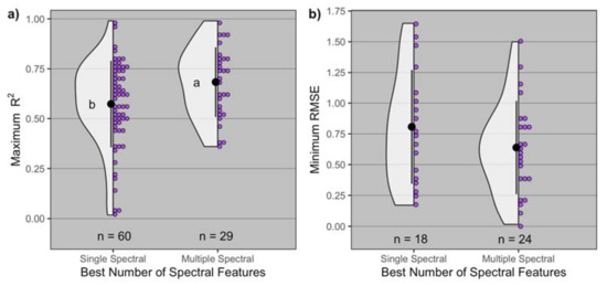
Figure 2.
Distribution of (a) maximum R2 and (b) minimum root mean squared error (RMSE) by type of the best spectral covariable (single and multiple spectral). Black dot and lines represent the mean ± standard deviation, and n is the number of observations for each best number of spectral features. In panel (a), means followed by the same letter are not significantly different at α = 0.05.
3.6. Type of Spectral Features
The spectral bands blue and green were identified as the most relevant features for modeling GPC for proximal and remote sensors and resulted in significant differences in maximum R2 and minimum RMSE, whereas other bands had no effect (Figure 3). The inclusion of the blue band resulted in an increased maximum R2 (0.76 on average), compared to when this band was not part of the best spectral feature (0.57 on average). The greatest maximum R2 observed when the blue band was present was 0.97 (id = 8), and when it was absent was 0.99 (id = 80) (Supplementary Table S1).
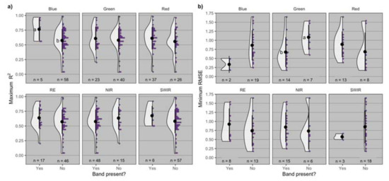
Figure 3.
Distribution of (a) maximum R2 and (b) minimum root mean squared error (RMSE) by presence or absence of different bands (blue, green, red, RE = red-edge, NIR = near infrared, SWIR = short wave infrared) in the spectral feature utilized to model grain protein concentration. Black dot and lines represent the mean ± standard deviation, and n is the number of observations for each distribution. Means followed by the same letter are not significantly different at α = 0.05.
The inclusion of the green band resulted in a decreased minimum RMSE (0.68% on average) compared to when this band was not part of the best spectral feature (1.1% on average). The least minimum RMSE observed when the green band was present was 0.17% (id = 8), and when it was absent was 0.1% (id = 39) (Supplementary Table S1).
3.7. Nonspectral Covariables
The number of spectral features (bands and/or vegetation indices), along with the inclusion of other covariables (e.g., weather, gluten category, mechanistic crop modeling) for proximal and remote sensors, resulted in significant differences in maximum R2 (p = 0.03, Supplementary Figure S1f). A single spectral feature alone had the lowest maximum R2 (0.56 on average) and was significantly different from multiple spectral (0.69 on average). The greatest maximum R2 for single spectral was 0.99 (id = 80), for single spectral plus other was 0.85 (id = 69), for multiple spectral was 0.99 (id = 63), and for multiple spectral plus other was 0.77 (id = 31a) (Table 1).
The number of spectral features, along with the inclusion of other covariables, resulted in similar minimum RMSE (p = 0.45, Supplementary Figure S1g) and varied from 0.58% to 0.85%, on average. The least minimum RMSE observed for single spectral was 0.17% (id = 8), for single spectral plus other was 0.34% (id = 68), for multiple spectral was 0.02% (id = 63), and for multiple spectral plus other was 0.4% (id = 31a) (Table 1).
3.8. Spectral Frequency
The best spectral frequency for proximal and remote sensors resulted in similar maximum R2 (p = 0.7, Supplementary Figure S1h) with accuracies of 0.61 for single and 0.59 for multiple dates, on average. The greatest maximum R2 observed for single date was 0.99 (ids = 63, 80), and for multiple dates was 0.89 (id = 38). The best spectral frequency resulted in similar minimum RMSE (p = 0.1, Supplementary Figure S1i), with single date precision of 0.66% and multiple dates precision of 0.92%, on average. The least minimum RMSE observed for single date was 0.02% (id = 63), and for multiple dates was 0.4% (id = 1a).
3.9. Statistical Approach
The statistical analysis approach for proximal and remote sensors resulted in significant differences in maximum R2 (p = 0.007), with model average maximum R2 increasing from 0.56 with simpler bivariate to 0.81 with complex RF-ANN models (Figure 4). The greatest maximum R2 observed for the bivariate family was 0.99 (id = 80), for the multivariate family was 0.85 (id = 69), for the PLSR family was 0.92 (id = 15), and for RF-ANN was 0.99 (id = 63) (Table 1).
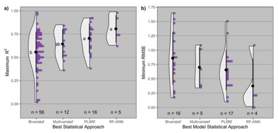
Figure 4.
Distribution of (a) maximum R2 and (b) minimum root mean squared error (RMSE) by statistical approach (bivariatef = bivariate family, multivariatef = multivariate family, PLSRf = partial least squares family, RF-ANN = random forest artificial neural network) utilized to model grain protein concentration. Black dot and lines represent the mean ± standard deviation, and n is the number of observations for each distribution of best statistical approach. Means followed by the same letter are not significantly different at α = 0.05.
The statistical analysis approach resulted in similar minimum RMSE (p = 0.18), ranging from 0.37% with RF-ANN models to 0.86% with bivariate models, on average (Figure 4). The least minimum RMSE observed for the bivariate family was 0.17% (id = 8), for the multivariate family was 0.34% (id = 68), for the PLSR family was 0.1% (id = 39), and for RF-ANN was 0.02% (id = 63) (Table 1).
4. Discussion
This synthesis analysis is the first attempt to summarize GPC prediction results across different sensor type studies based on GPC model accuracy and precision. Our work expands on the previous review published by [18] by (i) including both on- and off-combine sensors and comparing their performance in predicting GPC, (ii) identifying the most optimal off-combine sensing characteristics for creating a reliable GPC layer, and (iii) highlighting current limitations and laying the groundwork for future developments in GPC prediction.
Our study demonstrated that on-combine sensors are more accurate than remote sensors in predicting GPC, yet with similar precision. This is an important finding as it points to a tradeoff between GPC predictive performance (better with on-combine sensors) versus capacity for within season management, segregated harvest planning, and lower implementation cost (better with remote sensors). However, on-combine sensors can quickly become the “gold standard” for benchmarking in season prediction of GPC layer. These points are thoroughly discussed below.
Overall, off-combine GPC prediction accuracy was optimized when sensing near to anthesis, using more than one spectral feature comprised of the blue band along with complex statistical approaches. GPC prediction precision was optimized when sensing near anthesis and using a spectral feature comprised of the green band. Leaf N content at anthesis is correlated with GPC [46]. Sensing around this time provides information on the potential reservoir for N at canopy scale, an important source for protein formation via post-anthesis N remobilization to the grain [104]. Near anthesis, crop biomass generally surpasses the threshold of 2 leaf area index units above which the red band saturates and becomes insensitive to increasing biomass and chlorophyll levels [105,106]. Under conditions of high biomass and chlorophyll, replacing the red band with the green band in normalized difference vegetation indices has successfully been used to regain sensitivity of sensed data to crop reflectance [105], which can be related to the improved precision when using the green band observed in our study. Using both the green and blue bands in a normalized difference index had great GPC predictive accuracy and precision [41]. The authors attributed the success of combining both bands to their strong relationship with chlorophyll, carotenoids, and leaf N [41]. Further, the blue band has also been negatively correlated with biomass, leaf and plant water content, and GPC [48]. Thus, these bands can potentially contribute to improved GPC predictive power by combining information on both canopy level pigment concentration and water condition, two critical factors driving N uptake, remobilization, and GPC formation.
Our results point to the need of combining multiple vegetation indices with complex statistical analysis to assist in untangling intricate crop reflectance responses that are difficult to predict with fewer spectral features and simpler models. Complex statistical analysis, such as PLSR, RF and ANN, may result in improved model performance at the expense of interpretability. Optimizing predictive accuracy should be the main goal when creating GPC predictions, and only then should the issue of model interpretability be considered [107]. To address the lack of interpretability in GPC prediction from complex models, posthoc interpretability methods could be used to ensure predictions are evaluated within the context of their relevancy in addressing one or more specific uses of this technology [107].
The above guidelines provide a direction for future GPC sensing studies to increase the likelihood of creating accurate and precise GPC predictive models. Such models have been previously proposed to be utilized for (i) next season N fertilizer management, (ii) segregated harvest, and (iii) environmental compliance [18]. Within season remote sensing, we further propose new uses of a spatial GPC layer, including (iv) same season fertilizer management for increased GPC, and (v) in advance segregated harvest planning related to field prioritization and farm infrastructure.
Next season fertilizer N management can be assisted by the use of spatial GPC and grain yield layers to calculate N removal in the previous season, which is then utilized as the variable rate N layer to be applied in the following growing season in a monocropping system. Previous season GPC layer used for variable rate N has been demonstrated to maintain or increase wheat grain yield while maintaining or increasing GPC levels and net returns, compared to a fixed rate N management in semiarid regions [13,15]. Nonetheless, its applicability has neither been tested with different crop rotations nor in wider ranges of water availability, where in season weather drives crop growth, N response and GPC.
Same season N management for increased GPC can only be assisted by off-combine sensing, mainly via the utilization of remote sensing to improve scalability. For this, crop reflectance from in season sensing is transformed into a GPC layer, which is then used as a benchmark to calculate variable N fertilizer rates that, when applied economically, increase GPC at harvest. This approach would need to consider the yield potential of different zones of the field and the spatially differential relationships between grain yield and GPC [2,5]. This approach can benefit from the feedback from an at harvest on-combine GPC layer, providing the ground-truthing GPC data to improve the in season predictions (postmortem evaluation) and further adjust in season GPC predictive models.
Segregated harvest can be assisted by the use of a GPC layer created by both on- and off-combine sensors. When on-combine sensing is used, grain segregation occurs at the combine level, which requires a mounted GPC sensor and at least two separate grain bins, one for low and another for high protein grain [10]. The added hardware cost will be incurred by the producer, which could signify an earlier barrier for technology adoption, but when added to the cost of the machinery, then its general adoption will significantly expand over time. Moreover, since on-combine GPC sensing occurs in parallel with harvest, it does not allow for the preharvest assessment of GPC variability (within and across fields) for prioritization and planning purposes.
When off-combine sensing is used, especially if employed via remote sensors, the magnitude and extent of GPC variability across fields can be assessed and used to prioritize highly variable GPC fields for segregated harvest. Within a given field, GPC homogenous zones can be identified before harvest, and then harvested and stored separately. Finally, the preharvest GPC prediction gives the producer time to plan how to allocate grain storage capacity across different GPC harvest loads. As off-combine remote sensing does not require added hardware for sensing and grain segregation, it will be more cost-effective to a producer and prone to adoption. Nonetheless, formal validation of the level of agreement on the sensing should be performed by combining this data (off-combine) with the on-combine GPC layer.
An important aspect of GPC zoning is its temporal variability and predictability performance both in and across season. In season GPC prediction performance is expected to vary as crops grow, develop, undergo stresses, and senesce [26,84], and can be overcome by sensing fields at model optimized growth stages, such as near anthesis, as indicated by our results. Across season GPC prediction performance is directly affected by the temporal stability and persistence of GPC zones. Depending on crop, soil, weather, and management interactions, GPC zones can change not only in mean GPC value, but also in their spatial extent and location from one season to another [2,10,14,64]. To overcome this issue, GPC prediction maps need to be updated at least once every growing season. Studies are needed to evaluate the temporal stability and persistence of GPC zones both in and across season for multiple growing seasons, to elucidate how GPC changes spatially and temporally in the long term.
Environmental compliance can be assisted by the use of a GPC layer by providing information on spatial crop N removal, which, when combined with N inputs (e.g., fertilizer N rate), allows for the calculation of spatial N balance [17]. The larger the N balance, the more opportunity for environmental pollution via nitrate leaching and nitrous oxide emissions [16]. Thus, a spatial N balance layer can be used by the producer (i) to identify under and over fertilized zones and adjust N fertilization rates for the next crop in the rotation, and (ii) to demonstrate improvements in N balance and environmental stewardship to the general public [16].
Lastly, spatial GPC adoption for any one or more purposes will depend on farmers’ interest in the technology based on its return on investment. A recent survey of soybean farmers from multiple U.S. states identified that >55% of 186 respondents would be interested in investing in technology to assess spatial GPC if a premium level of at least $0.50 was paid per bushel when GPC was above a certain threshold [108]. Farmer interest is expected to increase, as both the direct and indirect benefits of a spatial GPC layer become more evident.
Limitations of the current study and the literature were identified related to (i) crop representativeness, (ii) GPC analysis, (iii) model training, (iv) model fit metric reporting, and (v) model implementation. A large majority of the studies (i.e., 85%) were conducted on wheat. The success of this technology will depend on how it can be applied to different crops and rotations, thus, more studies on a large variety of crop types are necessary.
Reliable ground-truth GPC data is the first step in creating a robust GPC predictive model, but this is a labor and cost intensive task. Most of the studies included in this work utilized laboratory near infra-red equipment to indirectly measure ground-truth GPC, yet very few studies reported on whether this equipment had been properly calibrated with a traditional chemical laboratory N analysis (e.g., Kjeldahl N analysis; [109]). Future studies should ensure that proper equipment calibration is conducted and report on its performance.
The majority of the studies reported model fit metrics computed on the same data used for training the model. This practice likely overestimates model accuracy and precision, building models that fit the training data well, but that have issues predicting new data correctly across different spatiotemporal scales (different fields for the same crop, and same crop but in other seasons). Future research directions should split the data set into training, validation, and testing, using the training and validation sets for creating the model [21,29], and the testing set to evaluate model transfer learning ability to different spatiotemporal scales.
This synthesis focused on R2 and RMSE to assess GPC prediction quality, as these were the most commonly reported model fit metrics. Assuming the ideal model would have null intercept, unity slope, and low variability, only RMSE responds as expected (i.e., increasing) as the actual GPC predictive model deviates from the ideal condition. On the other hand, R2 does not respond as intercept deviates from null, and in fact increases as slope deviates from unity, which is undesirable with predicted–observed relationships where a slope of unity is the desired outcome. Thus, we recommend future studies also report other model fit metrics, such as the concordance correlation coefficient [110]. This metric has the benefits of (i) responding to deviations from a null intercept and unity slope, (ii) being decomposable into precision and accuracy components, and (iii) the metric itself and its components of precision and accuracy can undergo significance testing [111,112].
Finally, all studies included in this synthesis reported creating a sensor based spatial GPC prediction, yet the majority of the studies lacked demonstrations of its implementation. This synthesis showed that a GPC layer can be created with reasonable accuracy and precision. Future studies should build on this finding, create reliable GPC predictions, implement the predicted GPC layer to any one or more uses, and test its performance against the conventional methods. This benchmarking will be key to elucidate the potential economic value of a spatial GPC layer across various uses and define the future of this technology.
5. Conclusions
This synthesis gathered and summarized 84 studies from the literature reporting the accuracy and/or precision of grain protein concentration predictive models. We found that on-combine sensors are more accurate than remote sensors, although both have similar precision. This has implications on the tradeoff between model performance versus model scalability and potential for decision-making planning. For off-combine sensors, we identified the most important sensing characteristics to create a reliable grain protein concentration model. Those included sensing near anthesis using multiple spectral features that include the blue and green bands, and that are analyzed by complex statistical approaches.
We contrasted and compared the use of different sensor types for the previously proposed uses of a grain protein concentration layer of (i) next-season N fertilizer management, (ii) segregated harvest, and (iii) environmental compliance. We further proposed two new uses of an in season grain protein concentration layer, namely, (iv) within season nitrogen management for increased grain protein concentration, and (v) in advance segregated harvest planning.
We identified current limitations of the technology and proposed directions to be explored by future research. Those included performing grain protein concentration predictive studies on a larger variety of crops and water regimes; performing and reporting proper grain protein concentration ground-truth calibrations; creating transferable grain protein concentration predictive models by conducting proper model training, validation, and testing; reporting model fit metrics that express greater concordance with the ideal predictive model and that can be partitioned into accuracy and precision; and implementing and benchmarking one or more uses for a grain protein concentration layer. Altogether, these research lines will assist in developing reliable grain protein concentration predictive capacity across diverse crops, environments, and management options, and will further elucidate the potential agronomic, economic, and environmental value of a grain protein concentration layer when implemented across multiple uses in a farming operation.
Supplementary Materials
The following are available online at https://www.mdpi.com/article/10.3390/rs13245027/s1, Figure S1: Best crop stage for grain protein concentration (GPC) prediction based on maximum R2 (a), and distribution of maximum R2 and minimum root mean squared error (RMSE) explained by spatial resolution of remote sensors (b,c), number of days sensed by proximal and remote sensors (d,e), best covariable type (f,g), and best spectral frequency (h,i). Here, n is the number of observations for each distribution. Black dot and lines represent the mean ± standard deviation. In panel (f), means followed by the same letter are not significantly different at α = 0.05. Table S1: Summary of the selected studies for the synthesis analysis, including entry identification, citation, crop, and sensor-specific characteristics including sensor type, spatial resolution, the best type of spectral feature and columns identifying whether the best type of spectral feature included or not the bands of blue (400–500 nm), green (500–600 nm), red (600–700 nm), red-edge (RE, 700–800 nm), near-infrared (NIR, 800–1300 nm), and short-wave infrared (1300–1900 nm), and grain protein concentration model fit metrics.
Author Contributions
Conceptualization, L.M.B., A.F.d.B.R. and I.A.C.; investigation, L.M.B. and A.F.d.B.R.; methodology, L.M.B., A.F.d.B.R. and I.A.C.; software, L.M.B.; validation, L.M.B., A.F.d.B.R. and I.A.C.; resources, I.A.C.; data Curation, L.M.B.; writing—original draft preparation, L.M.B., A.F.d.B.R. and I.A.C.; writing—review and editing, L.M.B., A.F.d.B.R., Y.W., A.S. and I.A.C.; visualization, L.M.B.; supervision, project administration and funding acquisition, I.A.C. All authors have read and agreed to the published version of the manuscript.
Funding
We thank the John Deere Company for providing financial support for Bastos’ stipend and Ciampitti research program in order to conduct this synthesis analysis.
Data Availability Statement
Data is contained within the article.
Acknowledgments
This is Contribution no. 22-137-J from the Kansas Agricultural Experiment Station.
Conflicts of Interest
Author Y.W. is employed by the company John Deere. The remaining authors declare that the research was conducted in the absence of any commercial or financial relationships that could be construed as a potential conflict of interest. The sponsors had no role in the design, execution, interpretation or writing of the study.
Abbreviations
| GPC | Grain protein concentration |
| N | Nitrogen |
| RMSE | Root mean squared error |
| PLSR | Partial least-square regression |
| RF | Random forest |
| ANN | Artificial neural network |
| CIT | Conditional inference tree |
| RE | Red-edge |
| NIR | Near infra-red |
| SWIR | Short-wave near-infrared |
References
- Delin, S. Within-field variations in grain protein content—relationships to yield and soil nitrogen and consistency in maps between years. Precis. Agric. 2004, 5, 565–577. [Google Scholar] [CrossRef]
- Long, D.S.; McCallum, J.D. On-combine, multi-sensor data collection for post-harvest assessment of environmental stress in wheat. Precis. Agric. 2015, 16, 492–504. [Google Scholar] [CrossRef]
- Norng, S.; Pettitt, A.; Kelly, R.; Butler, D.; Strong, W. Investigating the relationship between site-specific yield and protein of cereal crops. Precis. Agric. 2005, 6, 41–51. [Google Scholar] [CrossRef]
- Reyns, P.; Spaepen, P.; De Baerdemaeker, J. Site-specific relationship between grain quality and yield. Precis. Agric. 2000, 2, 231–246. [Google Scholar] [CrossRef]
- Whelan, B.M.; Taylor, J.A.; Hassall, J.A. Site-specific variation in wheat grain protein concentration and wheat grain yield measured on an Australian farm using harvester-mounted on-the-go sensors. Crop Pasture Sci. 2009, 60, 808–817. [Google Scholar] [CrossRef]
- Klem, K.; Záhora, J.; Zemek, F.; Trunda, P.; Tůma, I.; Novotná, K.; Hodaňová, P.; Rapantová, B.; Hanuš, J.; Vavříková, J.; et al. Interactive effects of water deficit and nitrogen nutrition on winter wheat. Remote sensing methods for their detection. Agric. Water Manag. 2018, 210, 171–184. [Google Scholar] [CrossRef]
- Long, D.S.; Carlson, G.R.; Engel, R.E. Grain protein mapping for precision management of dryland wheat. In Proceedings of the Fourth International Conference on Precision Agriculture, St. Paul, MN, USA, 19–22 July 1998; pp. 787–796. [Google Scholar]
- Engel, R.E.; Long, D.S.; Carlson, G.R.; Meirer, C. Method for precision nitrogen management in spring wheat: I fundamental relationships. Precis. Agric. 1999, 1, 327–338. [Google Scholar] [CrossRef]
- Morari, F.; Zanella, V.; Sartori, L.; Visioli, G.; Berzaghi, P.; Mosca, G. Optimising durum wheat cultivation in North Italy: Understanding the effects of site-specific fertilization on yield and protein content. Precis. Agric. 2018, 19, 257–277. [Google Scholar] [CrossRef]
- Basso, B.; Cammarano, D.; Chen, D.; Cafiero, G.; Amato, M.; Bitella, G.; Rossi, R.; Basso, F. Landscape position and precipitation effects on spatial variability of wheat yield and grain protein in Southern Italy. J. Agron. Crop Sci. 2009, 195, 301–312. [Google Scholar] [CrossRef]
- Kravchenko, A.N.; Bullock, D.G. Spatial variability of soybean quality data as a function of field topography: I. spatial data analysis. Crop Sci. 2002, 42, 804–815. [Google Scholar] [CrossRef]
- Stewart, C.M.; McBratney, A.B.; Skerritt, J.H. Site-specific durum wheat quality and its relationship to soil properties in a single field in Northern New South Wales. Precis. Agric. 2002, 3, 155–168. [Google Scholar] [CrossRef]
- Long, D.S.; McCallum, J.D.; Martin, C.T.; Capalbo, S. Net returns from segregating dark northern spring wheat by protein concentration during harvest. Agron. J. 2016, 108, 1503–1513. [Google Scholar] [CrossRef][Green Version]
- Long, D.S.; McCallum, J.D.; Scharf, P.A. Optical-mechanical system for on-combine segregation of wheat by grain protein concentration. Agron. J. 2013, 105, 1529–1535. [Google Scholar] [CrossRef][Green Version]
- Martin, C.T.; McCallum, J.D.; Long, D.S. A web-based calculator for estimating the profit potential of grain segregation by protein concentration. Agron. J. 2013, 105, 721–726. [Google Scholar] [CrossRef][Green Version]
- Miao, R.; Hennessy, D.A. Optimal protein segregation strategies for wheat growers. Can. J. Agric. Econ./Rev. Can. D’Agroecon. 2015, 63, 309–331. [Google Scholar] [CrossRef]
- Bonfil, D.; Mufradi, I.; Asido, S.; Long, D. Precision nitrogen management based on nitrogen removal in rainfed wheat. In Proceedings of the 9th International Conference on Precision Agriculture, Denver, CO, USA, 20–23 July 2008. [Google Scholar]
- Engel, R.E.; Long, D.S.; Carlson, G.R. Grain protein as a post-harvest index of nitrogen status for winter wheat in the Northern Great Plains. Can. J. Plant Sci. 2006, 86, 425–431. [Google Scholar] [CrossRef]
- Long, D.S.; Nielsen, G.A.; Henry, M.P.; Westcott, M.P. Remote sensing for Northern Plains precision agriculture. In Proceedings of the Space 2000, Albuquerque, NM, USA, 27 February–2 March 2000; American Society of Civil Engineers: Albuquerque, NM, USA, 2000; pp. 208–214. [Google Scholar]
- McLellan, E.L.; Cassman, K.G.; Eagle, A.J.; Woodbury, P.B.; Sela, S.; Tonitto, C.; Marjerison, R.D.; van Es, H.M. The nitrogen balancing act: Tracking the environmental performance of food production. BioScience 2018, 68, 194–203. [Google Scholar] [CrossRef] [PubMed]
- Taylor, J.; Whelan, B. On-The-Go Protein Monitoring: A Review. Available online: https://www.researchgate.net/profile/James-Taylor-58/publication/259655553_On-the-go_grain_quality_monitoring_A_review/links/0deec52d2c169e7641000000/On-the-go-grain-quality-monitoring-A-review.pdf (accessed on 29 December 2020).
- Diacono, M.; Rubino, P.; Montemurro, F. Precision nitrogen management of wheat. a review. Agron. Sustain. Dev. 2013, 33, 219–241. [Google Scholar] [CrossRef]
- Øvergaard, S.I.; Isaksson, T.; Korsaeth, A. Prediction of wheat yield and protein using remote sensors on plots—part i: Assessing near infrared model robustness for year and site variations. J. Infrared Spectrosc. 2013, 21, 117–131. [Google Scholar] [CrossRef]
- Barmeier, G.; Hofer, K.; Schmidhalter, U. Mid-season prediction of grain yield and protein content of spring barley cultivars using high-throughput spectral sensing. Eur. J. Agron. 2017, 90, 108–116. [Google Scholar] [CrossRef]
- Magney, T.S.; Eitel, J.U.H.; Huggins, D.R.; Vierling, L.A. Proximal NDVI derived phenology improves in-season predictions of wheat quantity and quality. Agric. For. Meteorol. 2016, 217, 46–60. [Google Scholar] [CrossRef]
- Hama, A.; Tanaka, K.; Mochizuki, A.; Tsuruoka, Y.; Kondoh, A. Estimating the protein concentration in rice grain using UAV imagery together with agroclimatic data. Agronomy 2020, 10, 431. [Google Scholar] [CrossRef]
- Sarkar, T.K.; Ryu, C.-S.; Kang, Y.-S.; Kim, S.-H.; Jeon, S.-R.; Jang, S.-H.; Park, J.-W.; Kim, S.-G.; Kim, H.-J. Integrating UAV Remote Sensing with GIS for Predicting Rice Grain Protein. J. Biosyst. Eng. 2018, 43, 148–159. [Google Scholar] [CrossRef]
- Rodrigues, F.A.; Blasch, G.; BlasDefournych, P.; Ortiz-Monasterio, J.I.; Schulthess, U.; Zarco-Tejada, P.J.; Taylor, J.A.; Gérard, B. Multi-temporal and spectral analysis of high-resolution hyperspectral airborne imagery for precision agriculture: Assessment of wheat grain yield and grain protein content. Remote Sens. 2018, 10, 930. [Google Scholar] [CrossRef] [PubMed]
- Ryu, C.; Suguri, M.; Iida, M.; Umeda, M.; Lee, C. Integrating remote sensing and GIS for prediction of rice protein contents. Precis. Agric. 2011, 12, 378–394. [Google Scholar] [CrossRef]
- Wang, K.; Huggins, D.R.; Tao, H. Rapid mapping of winter wheat yield, protein, and nitrogen uptake using remote and proximal sensing. Int. J. Appl. Earth Obs. Geoinf. 2019, 82, 101921. [Google Scholar] [CrossRef]
- Xu, X.; Teng, C.; Zhao, Y.; Du, Y.; Zhao, C.; Yang, G.; Jin, X.; Song, X.; Gu, X.; Casa, R.; et al. Prediction of wheat grain protein by coupling multisource remote sensing imagery and ECMWF data. Remote Sens. 2020, 12, 1349. [Google Scholar] [CrossRef]
- Meier, C.G. Protein Mapping Spring Wheat Using a Mobile Near-Infrared Sensor and Terrain Modeling. Ph.D. Thesis, Montana State University-Bozeman, College of Agriculture, Bozeman, MT, USA, 2004. [Google Scholar]
- Sharabiani, V.; Kassar, F.; Gilandeh, Y.; Ardabili, S. Application of soft computing methods and spectral reflectance data for wheat growth monitoring. Iraqi J. Agric. Sci. 2019, 50, 1064–1076. [Google Scholar]
- Zhao, C.; Liu, L.; Wang, J.; Huang, W.; Song, X.; Li, C.; Wang, Z. Methods and application of remote sensing to forecast wheat grain quality. In Proceedings of the IEEE International Geoscience and Remote Sensing Symposium, Anchorage, AK, USA, 20–24 September 2004; Volume 6, pp. 4008–4010. [Google Scholar]
- Basnet, B.B.; Apan, A.; Kelly, R.; Jensen, T.; Strong, W.; Butler, D. Relating satellite imagery with grain protein content. In Proceedings of the 2003 Spatial Sciences Institute Biennial Conference: Spatial Knowledge without Boundaries (SSC2003), Spatial Sciences Institute, Canberra, Australia, 22–27 September 2003; pp. 1–11. [Google Scholar]
- Li, C.; Wang, J.; Wang, Q.; Wang, D.; Song, X.; Wang, Y.; Huang, W. Estimating wheat grain protein content using multi-temporal remote sensing data based on partial least squares regression. J. Integr. Agric. 2012, 11, 1445–1452. [Google Scholar] [CrossRef]
- Øvergaard, S.I.; Isaksson, T.; Kvaal, K.; Korsaeth, A. Comparisons of two hand-held, multispectral field radiometers and a hyperspectral airborne imager in terms of predicting spring wheat grain yield and quality by means of powered partial least squares regression. J. Infrared Spectrosc. 2010, 18, 247–261. [Google Scholar] [CrossRef]
- R Core Team. R: A Language and Environment for Statistical Computing; R Foundation for Statistical Computing: Vienna, Austria, 2020. [Google Scholar]
- Hansen, P.M.; Jørgensen, J.R.; Thomsen, A. Predicting grain yield and protein content in winter wheat and spring barley using repeated canopy reflectance measurements and partial least squares regression. J. Agric. Sci. 2002, 139, 307–318. [Google Scholar] [CrossRef]
- Nutter, F.W.; Tylka, G.L.; Guan, J.; Moreira, A.J.D.; Marett, C.C.; Rosburg, T.R.; Basart, J.P.; Chong, C.S. Use of remote sensing to detect soybean cyst nematode-induced plant stress. J. Nematol. 2002, 34, 222–231. [Google Scholar]
- Wright, D.L.; Ritchie, G.; Rasmussen, V.; Ramsey, D.; Baker, D. Managing grain protein in wheat using remote sensing. Online J. Space Commun. 2003, 3, 1–12. [Google Scholar]
- Kelly, R.; Cooper, J.; Thomas, G.; Strong, W.; Butler, D.; Apan, A. Using a handheld multispectral radiometer to forecast grain protein in northern Australia. In Proceedings of the 4th International Crop Science Congress, Brisbane, Australia, 26 September–1 October 2004. [Google Scholar]
- Maertens, K.; Reyns, P.; De Baerdemaeker, J. On-line measurement of grain quality with NIR technology. Trans. ASAE 2004, 47, 1135–1140. [Google Scholar] [CrossRef]
- Wang, Z.J.; Wang, J.H.; Liu, L.Y.; Huang, W.J.; Zhao, C.J.; Wang, C.Z. Prediction of grain protein content in winter wheat (Triticum aestivum L.) using plant pigment ratio (PPR). Field Crop. Res. 2004, 90, 311–321. [Google Scholar] [CrossRef]
- Wells, N.; Kelly, R.; Phinn, S.; Apan, A.; Jensen, T.; Cooper, J.; Strong, W. Use of airborne hyperspectral imagery to determine quality of sorghum crops. In Proceedings of the 12th Australasian Remote Sensing and Photogrammetry Conference (ARSPC 2004), Causal Productions, Fremantle, Australia, 18–22 October 2004. [Google Scholar]
- Wright, D.L.; Rasmussen, V.P.; Ramsey, R.D.; Baker, D.J.; Ellsworth, J.W. Canopy reflectance estimation of wheat nitrogen content for grain protein management. GIScience Remote Sens. 2004, 41, 287–300. [Google Scholar] [CrossRef]
- Long, D.; Rosenthal, T. Evaluation of an on-combine wheat protein analyzer on Montana hard red spring wheat. Progress report. In Proceedings of the 5th European Conference on Precision Agriculture, Uppsala, Sweden, 9–12 June 2005; Zeltex, Inc.: Hagerstown, MD, USA, 2005; p. 21740. [Google Scholar]
- Long, D.S.; Engel, R.E.; Carpenter, F.M. On-combine sensing and mapping of wheat protein concentration. Crop Manag. 2005, 4, 1–9. [Google Scholar] [CrossRef]
- Zhao, C.; Liu, L.; Wang, J.; Huang, W.; Song, X.; Li, C. Predicting grain protein content of winter wheat using remote sensing data based on nitrogen status and water stress. Int. J. Appl. Earth Obs. Geoinf. 2005, 7, 1–9. [Google Scholar] [CrossRef]
- Apan, A.; Kelly, R.; Phinn, S.; Strong, W.; Lester, D.; Butler, D.; Robson, A. Predicting grain protein content in wheat using hyperspectral sensing of in-season crop canopies and partial least squares regression. Int. J. Geoinform. 2006, 2, 93–108. [Google Scholar]
- Liu, L.; Wang, J.; Bao, Y.; Huang, W.; Ma, Z.; Zhao, C. Predicting winter wheat condition, grain yield and protein content using multi-temporal EnviSat-ASAR and Landsat TM satellite images. Int. J. Remote Sens. 2006, 27, 737–753. [Google Scholar] [CrossRef]
- Long, D.S.; Baker, A. On-Combine Sensing of Grain Protein Concentration in Soft White Winter Wheat. 2006 Dryland Agricultural Annual Report. 2006, pp. 18–24. Available online: https://nanopdf.com/download/2006-dryland-agricultural-annual-report-aig-special-report-1068_pdf (accessed on 16 November 2021).
- Pettersson, C.-G.; Söderström, M.; Eckersten, H. Canopy reflectance, thermal stress, and apparent soil electrical conductivity as predictors of within-field variability in grain yield and grain protein of malting barley. Precis. Agric. 2006, 7, 343–359. [Google Scholar] [CrossRef]
- Reyniers, M.; Vrindts, E.; De Baerdemaeker, J. Comparison of an aerial-based system and an on the ground continuous measuring device to predict yield of winter wheat. Eur. J. Agron. 2006, 24, 87–94. [Google Scholar] [CrossRef]
- Jensen, T.; Apan, A.; Young, F.; Zeller, L. Detecting the attributes of a wheat crop using digital imagery acquired from a low-altitude platform. Comput. Electron. Agric. 2007, 59, 66–77. [Google Scholar] [CrossRef]
- Pettersson, C.G.; Eckersten, H. Prediction of grain protein in spring malting barley grown in Northern Europe. Eur. J. Agron. 2007, 27, 205–214. [Google Scholar] [CrossRef]
- Xue, L.-H.; Cao, W.-X.; Yang, L.-Z. Predicting grain yield and protein content in winter wheat at different N supply levels using canopy reflectance spectra. Pedosphere 2007, 17, 646–653. [Google Scholar] [CrossRef]
- Huang, W.; Song, X.; Lamb, D.W.; Wang, Z.; Niu, Z.; Liu, L.; Wang, J. Estimation of winter wheat grain crude protein content from in situ reflectance and advanced spaceborne thermal emission and reflection radiometer image. J. Appl. Remote Sens. 2008, 2, 023530. [Google Scholar] [CrossRef]
- Long, D.S.; Engel, R.E.; Siemens, M.C. Measuring grain protein concentration with in-line near infrared reflectance spectroscopy. Agron. J. 2008, 100, 247–252. [Google Scholar] [CrossRef]
- Papale, D.; Belli, C.; Gioli, B.; Miglietta, F.; Ronchi, C.; Vaccari, F.; Valentini, R. ASPIS, a flexible multispectral system for airborne remote sensing environmental applications. Sensors 2008, 8, 3240–3256. [Google Scholar] [CrossRef]
- Fox, G.P.; Bloustein, G.; Sheppard, J. “On-the-go” NIT technology to assess protein and moisture during harvest of wheat breeding trials. J. Cereal Sci. 2010, 51, 171–173. [Google Scholar] [CrossRef]
- Qualm, A.M.; Osborne, S.L.; Gelderman, R. Utilizing existing sensor technology to predict spring wheat grain nitrogen concentration. Commun. Soil Sci. Plant Anal. 2010, 41, 2086–2099. [Google Scholar] [CrossRef]
- Risius, H.; Hahn, J.; Korte, H. Monitoring of Grain Quality and Segregation of Grain According to Protein Concentration Threshold on an Operating Combine Harvester. Book of Abstracts, Proceedings of the XVIIth World Congress of the International Commission of Agricultural and Biosystems Engineering (CIGR|SCGAB), Québec City, QC, Canada, 13–17 June 2010; Canadian Society for Bioengineering: Québec City, QC, Canada, 2010; p. 28. Available online: https://www.semanticscholar.org/paper/Monitoring-of-grain-quality-and-segregation-of-to-Risius-Hahn/3573ee9ba88e1c3a5c466294714314a0c1dea24c (accessed on 16 November 2021).
- Söderström, M.; Börjesson, T.; Pettersson, C.-G.; Nissen, K.; Hagner, O. Prediction of protein content in malting barley using proximal and remote sensing. Precis. Agric. 2010, 11, 587–599. [Google Scholar] [CrossRef]
- Song, X.; Wang, J.; Huang, W. Winter Wheat Growth and Grain Protein Uniformity Monitoring through Remotely Sensed Data. In Proceedings of the Remote Sensing for Agriculture, Ecosystems and Hydrology XII. International Society for Optics and Photonics, Toulouse, France, 7 October 2010; Volume 7824, p. 78242G. [Google Scholar]
- Guasconi, F.; Dalla Marta, A.; Grifoni, D.; Mancini, M.; Orlando, F.; Orlandini, S. Influence of climate on durum wheat production and use of remote sensing and weather data to predict quality and quantity of harvests. J. Agrometeorol. 2011, 3, 21–28. [Google Scholar]
- Han-ya, I.; Ishii, K.; Noguchi, N. Rice yields and protein content estimation by low-altitude remote sensing using spectroradiometer. IFAC Proc. Vol. 2011, 44, 1796–1801. [Google Scholar] [CrossRef]
- Onoyama, H.; Ryu, C.; Suguri, M.; Iida, M. Estimation of rice protein content using ground-based hyperspectral remote sensing. Eng. Agric. Environ. Food 2011, 4, 71–76. [Google Scholar] [CrossRef]
- Orlandini, S.; Mancini, M.; Grifoni, D.; Orlando, F.; Dalla Marta, A.; Capecchi, V. Integration of meteo-climatic and remote sensing information for the analysis of durum wheat quality in Val d’Orcia (Tuscany, Italy). Q. J. Hung. Meteorol. Serv. 2011, 115, 233–245. [Google Scholar]
- Zhang, J.; Gu, X.; Wang, J.; Huang, W.; Dong, Y.; Luo, J.; Yuan, L.; Li, Y. Evaluating maize grain quality by continuous wavelet analysis under normal and lodging circumstances. Sens. Lett. 2012, 10, 580–585. [Google Scholar] [CrossRef]
- Schoch, A.S. Enhanching Protein Concentration in Hard Red Spring Wheat with Nitrogen Management Based on Plant Predictors. Ph.D. Thesis, North Dakota State University, Fargo, ND, USA, 2013. [Google Scholar]
- Feng, M.; Xiao, L.; Zhang, M.; Yang, W.; Ding, G. Integrating remote sensing and GIS for prediction of winter wheat (triticum aestivum) protein contents in Linfen (Shanxi), China. PLoS ONE 2014, 9, e80989. [Google Scholar] [CrossRef]
- Xiu-liang, J.; Xin-gang, X.; Feng, H.; Xiao-yu, S.; Wang, Q.; Ji-hua, W.; Wen-shan, G. Estimation of grain protein content in winter wheat by using three methods with hyperspectral data. Int. J. Agric. Biol. 2014, 16, 498–504. [Google Scholar]
- Macnack, N.; Khim, B.C.; Mullock, J.; Raun, W. In-season prediction of nitrogen use efficiency and grain protein in winter wheat (Triticum aestivum L.). Commun. Soil Sci. Plant Anal. 2014, 45, 2480–2494. [Google Scholar] [CrossRef]
- Song, X.; Wang, J.; Yang, G.; Feng, H. Winter wheat cropland grain protein content evaluation through remote sensing. Intell. Autom. Soft Comput. 2014, 20, 599–609. [Google Scholar] [CrossRef]
- Wang, L.; Tian, Y.; Yao, X.; Zhu, Y.; Cao, W. Predicting grain yield and protein content in wheat by fusing multi-sensor and multi-temporal remote-sensing images. Field Crop. Res. 2014, 164, 178–188. [Google Scholar] [CrossRef]
- Xu, X.-G.; Li, C.-J.; Dong, Y.-S.; Song, X.-Y.; Jin, X.-L. Estimating grain protein content in winter wheat with multi-temporal hyperspectral measurements. Sens. Lett. 2014, 12, 855–859. [Google Scholar] [CrossRef]
- Li, Z.; Jin, X.; Zhao, C.; Wang, J.; Xu, X.; Yang, G.; Li, C.; Shen, J. Estimating wheat yield and quality by coupling the DSSAT-CERES model and proximal remote sensing. Eur. J. Agron. 2015, 71, 53–62. [Google Scholar] [CrossRef]
- Li, Z.; Wang, J.; Xu, X.; Zhao, C.; Jin, X.; Yang, G.; Feng, H. Assimilation of two variables derived from hyperspectral data into the DSSAT-CERES model for grain yield and quality estimation. Remote Sens. 2015, 7, 12400–12418. [Google Scholar] [CrossRef]
- Orlando, F.; Marta, A.D.; Mancini, M.; Motha, R.; Qu, J.J.; Orlandini, S. Integration of remote sensing and crop modeling for the early assessment of durum wheat harvest at the field scale. Crop Sci. 2015, 55, 1280–1289. [Google Scholar] [CrossRef]
- Geipel, J.; Link, J.; Wirwahn, J.; Claupein, W. A programmable aerial multispectral camera system for in-season crop biomass and nitrogen content estimation. Agriculture 2016, 6, 4. [Google Scholar] [CrossRef]
- Mengmeng, D.; Noboru, N.; Atsushi, I.; Yukinori, S. Multi-temporal monitoring of wheat growth by using images from satellite and unmanned aerial vehicle. Int. J. Agric. Biol. Eng. 2017, 10, 1–13. [Google Scholar] [CrossRef]
- Rellaford, M.J. Predicting and Enhancing Spring Wheat Grain Protein Content through Sensing and In-Season Nitrogen Fertilization. Ph.D. Thesis, North Dakota State University, Fargo, ND, USA, 2018. [Google Scholar]
- Prey, L.; Schmidhalter, U. Simulation of satellite reflectance data using high-frequency ground based hyperspectral canopy measurements for in-season estimation of grain yield and grain nitrogen status in winter wheat. ISPRS J. Photogramm. Remote Sens. 2019, 149, 176–187. [Google Scholar] [CrossRef]
- Zhao, H.; Song, X.; Yang, G.; Li, Z.; Zhang, D.; Feng, H. Monitoring of nitrogen and grain protein content in winter wheat based on Sentinel-2a data. Remote Sens. 2019, 11, 1724. [Google Scholar] [CrossRef]
- Aranguren, M.; Castellón, A.; Aizpurua, A. Crop sensor based non-destructive estimation of nitrogen nutritional status, yield, and grain protein content in wheat. Agriculture 2020, 10, 148. [Google Scholar] [CrossRef]
- Chen, P. Estimation of winter wheat grain protein content based on multisource data assimilation. Remote Sens. 2020, 12, 3201. [Google Scholar] [CrossRef]
- Li, Z.; Taylor, J.; Yang, H.; Casa, R.; Jin, X.; Li, Z.; Song, X.; Yang, G. A hierarchical interannual wheat yield and grain protein prediction model using spectral vegetative indices and meteorological data. Field Crop. Res. 2020, 248, 107711. [Google Scholar] [CrossRef]
- Long, D.S.; McCallum, J.D. Adapting a relatively low-cost reflectance spectrometer for on-combine sensing of grain protein concentration. Comput. Electron. Agric. 2020, 174, 105467. [Google Scholar] [CrossRef]
- Tan, C.; Zhou, X.; Zhang, P.; Wang, Z.; Wang, D.; Guo, W.; Yun, F. Predicting grain protein content of field-grown winter wheat with satellite images and partial least square algorithm. PLoS ONE 2020, 15, e0228500. [Google Scholar] [CrossRef] [PubMed]
- Walsh, O.S.; Torrion, J.A.; Liang, X.; Shafian, S.; Yang, R.; Belmont, K.M.; McClintick-Chess, J.R. Grain yield, quality, and spectral characteristics of wheat grown under varied nitrogen and irrigation. Agrosyst. Geosci. Environ. 2020, 3, e20104. [Google Scholar] [CrossRef]
- Aranguren, M.; Castellón, A.; Aizpurua, A. Wheat grain protein content under Mediterranean conditions measured with chlorophyll meter. Plants 2021, 10, 374. [Google Scholar] [CrossRef] [PubMed]
- Chiozza, M.V.; Parmley, K.A.; Higgins, R.H.; Singh, A.K.; Miguez, F.E. Comparative prediction accuracy of hyperspectral bands for different soybean crop variables: From leaf area to seed composition. Field Crop. Res. 2021, 271, 108260. [Google Scholar] [CrossRef]
- Kang, Y.; Nam, J.; Kim, Y.; Lee, S.; Seong, D.; Jang, S.; Ryu, C. Assessment of regression models for predicting rice yield and protein content using unmanned aerial vehicle-based multispectral imagery. Remote Sens. 2021, 13, 1508. [Google Scholar] [CrossRef]
- Kizilgeci, F.; Yildirim, M.; Islam, M.S.; Ratnasekera, D.; Iqbal, M.A.; Sabagh, A.E. Normalized difference vegetation index and chlorophyll content for precision nitrogen management in durum wheat cultivars under semi-arid conditions. Sustainability 2021, 13, 3725. [Google Scholar] [CrossRef]
- Sandhu, K.S.; Mihalyov, P.D.; Lewien, M.J.; Pumphrey, M.O.; Carter, A.H. Combining genomic and phenomic information for predicting grain protein content and grain yield in spring wheat. Front. Plant Sci. 2021, 12, 613300. [Google Scholar] [CrossRef] [PubMed]
- Santaga, F.S.; Benincasa, P.; Toscano, P.; Antognelli, S.; Ranieri, E.; Vizzari, M. Simplified and advanced Sentinel-2-based precision nitrogen management of wheat. Agronomy 2021, 11, 1156. [Google Scholar] [CrossRef]
- Savaşlı, E.; Karaduman, Y.; Önder, O.; Ateş, Ö. Prediction of grain protein content and gluten quality of bread wheat in the early vegetation period by optical sensors. J. Cereal Sci. 2021, 102, 103354. [Google Scholar] [CrossRef]
- Veverka, D.; Chatterjee, A.; Carlson, M. Comparisons of sensors to predict spring wheat grain yield and protein content. Agron. J. 2021, 113, 2091–2101. [Google Scholar] [CrossRef]
- Wang, Z.; Chen, J.; Zhang, J.; Fan, Y.; Cheng, Y.; Wang, B.; Wu, X.; Tan, X.; Tan, T.; Li, S.; et al. Predicting grain yield and protein content using canopy reflectance in maize grown under different water and nitrogen levels. Field Crop. Res. 2021, 260, 107988. [Google Scholar] [CrossRef]
- Zhou, X.; Kono, Y.; Win, A.; Matsui, T.; Tanaka, T.S.T. Predicting within-field variability in grain yield and protein content of winter wheat using UAV-based multispectral imagery and machine learning approaches. Plant Prod. Sci. 2021, 24, 137–151. [Google Scholar] [CrossRef]
- Fu, Z.; Yu, S.; Zhang, J.; Xi, H.; Gao, Y.; Lu, R.; Zheng, H.; Zhu, Y.; Cao, W.; Liu, X. Combining UAV multispectral imagery and ecological factors to estimate leaf nitrogen and grain protein content of wheat. Eur. J. Agron. 2022, 132, 126405. [Google Scholar] [CrossRef]
- Zaman, W. JCR, SCI Complete List of Journal Reports 2020. 2020. Available online: https://www.scribd.com/document/476514395/ImpactfactorandJIFQuartilereleasedon29june2020-pdf (accessed on 16 November 2021).
- Austin, R.B.; Ford, M.A.; Edrich, J.A.; Blackwell, R.D. The nitrogen economy of winter wheat. J. Agric. Sci. 1977, 88, 159–167. [Google Scholar] [CrossRef]
- Gitelson, A.A.; Kaufman, Y.J.; Merzlyak, M.N. Use of a green channel in remote sensing of global vegetation from EOS-MODIS. Remote Sens. Environ. 1996, 58, 289–298. [Google Scholar] [CrossRef]
- Gitelson, A.A.; Merzlyak, M.N. Remote estimation of chlorophyll content in higher plant leaves. Int. J. Remote Sens. 1997, 18, 2691–2697. [Google Scholar] [CrossRef]
- Murdoch, W.J.; Singh, C.; Kumbier, K.; Abbasi-Asl, R.; Yu, B. Definitions, methods, and applications in interpretable machine learning. Proc. Natl. Acad. Sci. USA 2019, 116, 22071–22080. [Google Scholar] [CrossRef]
- Diacono, M.; Castrignanò, A.; Troccoli, A.; De Benedetto, D.; Basso, B.; Rubino, P. Spatial and temporal variability of wheat grain yield and quality in a Mediterranean environment: A multivariate geostatistical approach. Field Crop. Res. 2012, 131, 49–62. [Google Scholar] [CrossRef]
- Brown, C. Achieving Soybean Seed Quality Is a Combination of Nature and Nurture. Available online: https://soybeanresearchinfo.com/research-highlight/achieving-soybean-seed-quality-is-a-combination-of-nature-and-nurture/ (accessed on 19 December 2020).
- Kirk, P.L. Kjeldahl method for total nitrogen. Anal. Chem. 1950, 22, 354–358. [Google Scholar] [CrossRef]
- Lin, L.I.-K. A concordance correlation coefficient to evaluate reproducibility. Biometrics 1989, 45, 255–268. [Google Scholar] [CrossRef] [PubMed]
- Lin, L.; Hedayat, A.S.; Sinha, B.; Yang, M. Statistical methods in assessing agreement: Models, issues, and tools. J. Am. Stat. Assoc. 2002, 97, 257–270. [Google Scholar] [CrossRef]


Publisher’s Note: MDPI stays neutral with regard to jurisdictional claims in published maps and institutional affiliations. |
© 2021 by the authors. Licensee MDPI, Basel, Switzerland. This article is an open access article distributed under the terms and conditions of the Creative Commons Attribution (CC BY) license (https://creativecommons.org/licenses/by/4.0/).