
Global Intercomparison of Hyper-Resolution ECOSTRESS Coastal Sea Surface Temperature Measurements from the Space Station with VIIRS-N20


Abstract
:1. Introduction
2. Materials and Methods
2.1. Data Acquisition and Processing
2.2. Spatial Autocorrelation and Brightness Temperature Corrections
2.3. Algorithm Selection
| SST = a0 + a1 BT11 + a2 ΔTFG + a3 ΔT + a4 ΔT SΘ | (NAVO) | (1) |
| SST = a0 + a1 BT11 + a2 ΔT + a3 ΔT SΘ + a4FG | (NRL) | (2) |
| SST = a0 + a1 BT11 + a2 ΔT+ a3 ΔTFG + a4 BT11 SΘ + a5 ΔT SΘ + a6 ZA | (NLSST) | (3) |
| SST = a0 + a1 BT11 + a2 ΔT +a3 ΔT SΘ | (MC) | (4) |
| SST = a0 + a1 BT11 + a2 ΔTFG + a3 SΘ+ a4 ZA + a5 ZA2 | (VIIRS) | (5) |
3. Results
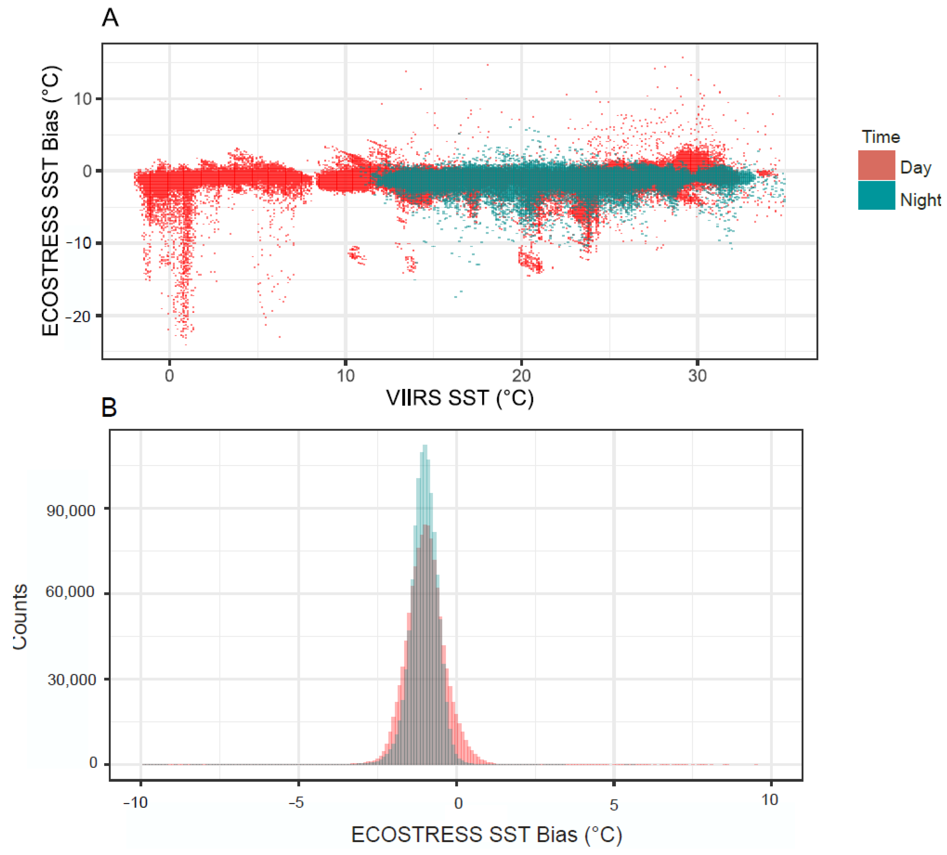
3.1. Bias Estimates
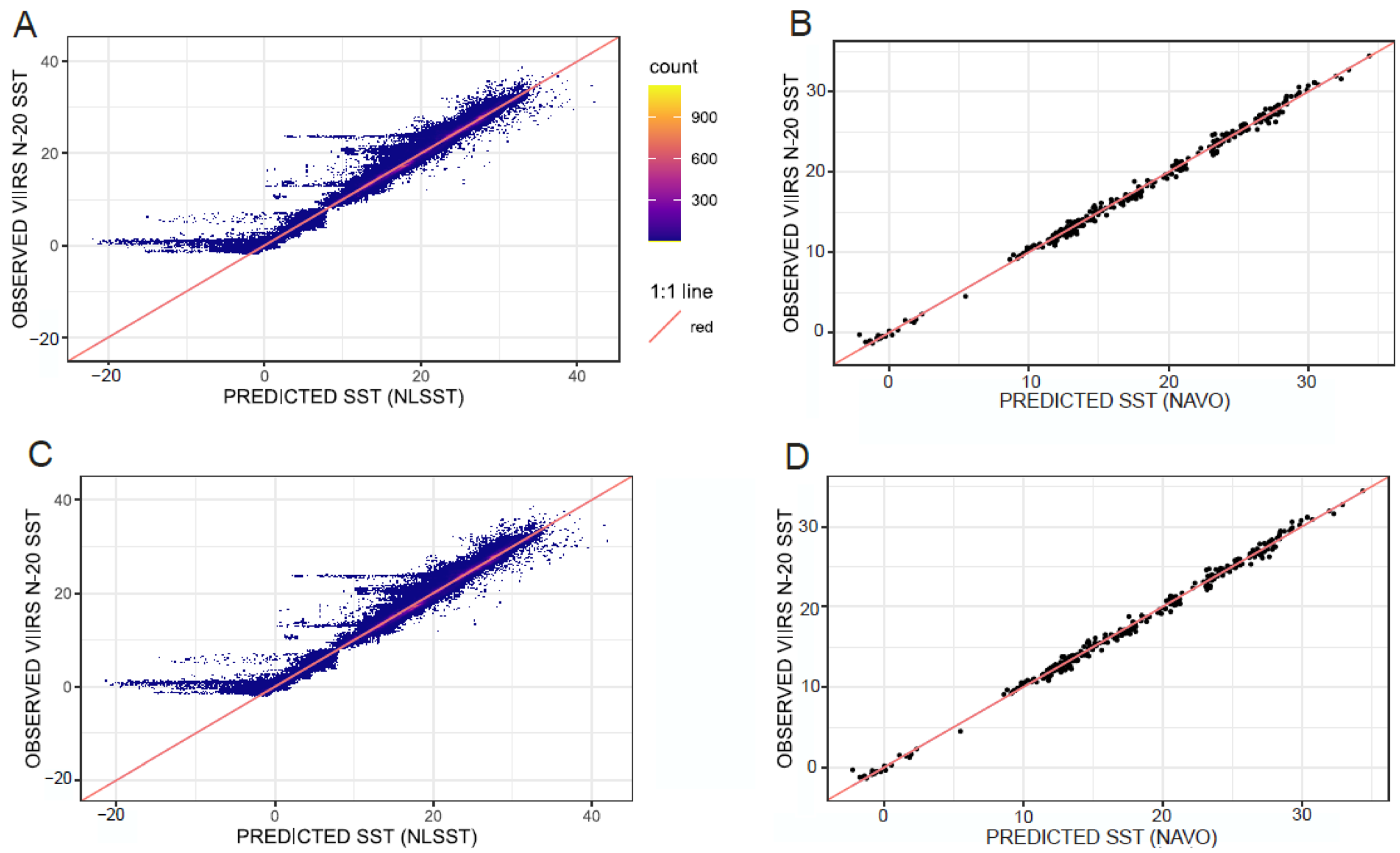
3.2. Spatial Autocorrelation Distances and Algorithm Selection
4. Discussion
4.1. Bias Magnitude and Nature
4.2. Biological and Oceanographic Implications of SST Bias
4.3. Importance of Spatial Autocorrelation in Algorithm Selection
5. Conclusions
Supplementary Materials
Author Contributions
Funding
Institutional Review Board Statement
Informed Consent Statement
Data Availability Statement
Acknowledgments
Conflicts of Interest
References
- Levitus, S.; Antonov, J.I.; Boyer, T.P.; Baranova, O.K.; Garcia, H.E.; Locarnini, R.A.; Mishonov, A.V.; Reagan, J.R.; Seidov, D.; Yarosh, E.S.; et al. World Ocean Heat Content and Thermosteric Sea Level Change (0–2000 m), 1955–2010. Geophys. Res. Lett. 2012, 39, L10603. [Google Scholar] [CrossRef] [Green Version]
- Alexander, L.V.; Allen, S.K.; Bindoff, N.L.; Bréon, F.-M.; Church, J.A.; Cubasch, U.; Emori, S.; Forster, P.; Friedlingstein, P.; Gillett, N.; et al. Climate Change 2013: The Physical Science Basis: Summary for Policymakers, a Report of Working Group I to the Fifth Assessment Report of the IPCC; Stocker, T., Qin, D., Plattner, G.K., Tignor, M., Allen, S.K., Boschung, J., Nauels, A., Xia, Y., Bex, V., Midgley, P.M., Eds.; Cambridge University Press: Cambridge, UK; New York, NY, USA, 2013; p. 1535. Available online: https://www.ipcc.ch/site/assets/uploads/2018/02/WG1AR5_SPM_FINAL.pdf (accessed on 7 December 2021).
- Baringer, M.; Bif, M.B.; Boyer, T.; Bushinsky, S.M.; Carter, B.R.; Cetinić, I.; Chambers, D.P.; Cheng, L.; Chiba, S.; Dai, M.; et al. Global Oceans. Bull. Am. Meteorol. Soc. 2020, 101, S129–S184. [Google Scholar] [CrossRef]
- Johnson, G.C.; Lyman, J.M. Warming Trends Increasingly Dominate Global Ocean. Nat. Clim. Chang. 2020, 10, 757–761. [Google Scholar] [CrossRef]
- Gruber, N.; Clement, D.; Carter, B.R.; Feely, R.A.; van Heuven, S.; Hoppema, M.; Ishii, M.; Key, R.M.; Kozyr, A.; Lauvset, S.K.; et al. The Oceanic Sink for Anthropogenic CO2 from 1994 to 2007. Science 2019, 363, 1193–1199. [Google Scholar] [CrossRef] [PubMed] [Green Version]
- Dangendorf, S.; Marcos, M.; Wöppelmann, G.; Conrad, C.P.; Frederikse, T.; Riva, R. Reassessment of 20th Century Global Mean Sea Level Rise. Proc. Natl. Acad. Sci. USA 2017, 114, 5946–5951. [Google Scholar] [CrossRef] [PubMed] [Green Version]
- Kulp, S.A.; Strauss, B.H. New Elevation Data Triple Estimates of Global Vulnerability to Sea-Level Rise and Coastal Flooding. Nat. Commun. 2019, 10, 4844. [Google Scholar] [CrossRef] [PubMed] [Green Version]
- Reguero, B.G.; Losada, I.J.; Méndez, F.J. A Recent Increase in Global Wave Power as a Consequence of Oceanic Warming. Nat. Commun. 2019, 10, 205. [Google Scholar] [CrossRef] [PubMed] [Green Version]
- Legeckis, R.; Gordon, A.L. Satellite Observation of the Brazil and Fakland Currents-1975 to 1976 and 1978. Deep Sea Res. 1982, 3A, 375–401. [Google Scholar] [CrossRef]
- Minnett, P.J.; Kilpatrick, K.A.; Podestá, G.P.; Evans, R.H.; Szczodrak, M.D.; Izaguirre, M.A.; Williams, E.J.; Walsh, S.; Reynolds, R.M.; Bailey, S.W.; et al. Skin Sea-Surface Temperature from VIIRS on Suomi-NPP—NASA Continuity Retrievals. Remote Sens. 2020, 12, 3369. [Google Scholar] [CrossRef]
- Emery, W.J.; Castro, S.; Wick, G.A.; Schluessel, P. Estimating sea surface temperature from infrared satellite and in situ temperature data. Bull. Am. Meteorol. Soc. 2001, 82, 2773–2786. [Google Scholar] [CrossRef] [Green Version]
- Schloesser, F.; Cornillon, P.; Donohue, K. Evaluation of Termosalinograph and VIIRS Data for the Characterization of Near Surface Temperature Fields. J. Atmos. Ocean. Tecnol. 2016, 33, 1843–1858. [Google Scholar] [CrossRef] [Green Version]
- Li, X.; Pichel, W.; Clemente-Colón, P.; Krasnopolsky, V.; Sapper, J. Validation of Coastal Sea and Lake Surface Temperature Measurements Derived from NOAA/AVHRR Data. Int. J. Remote Sens. 2001, 22, 1285–1303. [Google Scholar] [CrossRef]
- Zhang, H.-M. Bias Characteristics in the AVHRR Sea Surface Temperature. Geophys. Res. Lett. 2004, 31, L01307. [Google Scholar] [CrossRef]
- Lima, F.P.; Wethey, D.S. Three Decades of High-Resolution Coastal Sea Surface Temperatures Reveal More than Warming. Nat. Commun. 2012, 3, 704. [Google Scholar] [CrossRef] [PubMed] [Green Version]
- Bakun, A.; Black, B.A.; Bograd, S.J.; García-Reyes, M.; Miller, A.J.; Rykaczewski, R.R.; Sydeman, W.J. Anticipated Effects of Climate Change on Coastal Upwelling Ecosystems. Curr. Clim. Chang. Rep. 2015, 1, 85–93. [Google Scholar] [CrossRef] [Green Version]
- Seabra, R.; Varela, R.; Santos, A.M.; Gómez-Gesteira, M.; Meneghesso, C.; Wethey, D.S.; Lima, F.P. Reduced nearshore warming associated with eastern boundary upwelling systems. Front. Mar. Sci. 2019, 6, 104. [Google Scholar] [CrossRef] [Green Version]
- Canales, T.M.; Lima, M.; Wiff, R.; Contreras-Reyes, J.E.; Cifuentes, U.; Montero, J. Endogenous, Climate, and Fishing Influences on the Population Dynamics of Small Pelagic Fish in the Southern Humboldt Current Ecosystem. Front. Mar. Sci. 2020, 7, 82. [Google Scholar] [CrossRef]
- Bakun, A. Global Climate Change and Intensification of Coastal Upwelling. Science 1990, 247, 198–201. [Google Scholar] [CrossRef] [Green Version]
- Cordeiro Pires, A.; Nolasco, R.; Rocha, A.; Ramos, A.M.; Dubert, J. Climate Change in the Iberian Upwelling System: A Numerical Study Using GCM Downscaling. Clim. Dyn. 2016, 47, 451–464. [Google Scholar] [CrossRef]
- Sousa, M.C.; Ribeiro, A.; Des, M.; Gomez-Gesteira, M.; deCastro, M.; Dias, J.M. NW Iberian Peninsula Coastal Upwelling Future Weakening: Competition between Wind Intensification and Surface Heating. Sci. Total Environ. 2020, 703, 134808. [Google Scholar] [CrossRef]
- García-Reyes, M.; Largier, J. Observations of Increased Wind-Driven Coastal Upwelling off Central California. J. Geophys. Res. 2010, 115, C04011. [Google Scholar] [CrossRef] [Green Version]
- Weidberg, N.; Ospina-Alvarez, A.; Bonicelli, J.; Barahona, M.; Aiken, C.M.; Broitman, B.R.; Navarrete, S.A. Spatial Shifts in Productivity of the Coastal Ocean over the Past Two Decades Induced by Migration of the Pacific Anticyclone and Bakun’s Effect in the Humboldt Upwelling Ecosystem. Glob. Planet. Chang. 2020, 193, 103259. [Google Scholar] [CrossRef]
- Hulley, G.C.; Hook, S.J. Level 2 Land Surface Temperature and Emissivity Algorithm Theoretical Basis Document (ATBD). NASA JPL Rep. 2015. Available online: https://ecostress.jpl.nasa.gov/downloads/atbd/ECOSTRESS_L2_ATBD_LSTE_2018-03-08.pdf (accessed on 7 December 2021).
- Hulley, G.C.; Göttsche, F.M.; Rivera, G.; Hook, S.J.; Freepartner, R.J.; Martin, M.A.; Cawse-Nicholson, K.; Johnson, W.R. Validation and Quality Assessment of the ECOSTRESS Level-2 Land Surface Temperature and Emissivity Product. IEEE Trans. Geosci. Remote Sens. 2021, 1–23. [Google Scholar] [CrossRef]
- Hook, S.J.; Cawse-Nicholson, K.; Barsi, J.; Radocinski, R.; Hulley, G.C.; Johnson, W.R.; Rivera, G.; Markham, B. In-Flight Validation of the ECOSTRESS, Landsats 7 and 8 Thermal Infrared Spectral Channels Using the Lake Tahoe CA/NV and Salton Sea CA Automated Validation Sites. IEEE Trans. Geosci. Remote Sens. 2020, 58, 1294–1302. [Google Scholar] [CrossRef]
- Shi, J.; Hu, C. Evaluation of ECOSTRESS Thermal Data over South Florida Estuaries. Sensors 2021, 21, 4341. [Google Scholar] [CrossRef]
- Xiong, X.; Angal, A.; Chang, T.; Chiang, K.; Lei, N.; Li, Y.; Sun, J.; Twedt, K.; Wu, A. MODIS and VIIRS Calibration and Characterization in Support of Producing Long-Term High-Quality Data Products. Remote Sens. 2020, 12, 3167. [Google Scholar] [CrossRef]
- Wang, W.; Cao, C. Monitoring the NOAA Operational VIIRS RSB and DNB Calibration Stability Using Monthly and Semi-Monthly Deep Convective Clouds Time Series. Remote Sens. 2016, 8, 32. [Google Scholar] [CrossRef] [Green Version]
- Cao, C.; Xiong, J.; Blonski, S.; Liu, Q.; Uprety, S.; Shao, X.; Bai, Y.; Weng, F. Suomi NPP VIIRS Sensor Data Record Verification, Validation, and Long-Term Performance Monitoring. J. Geophys. Res. Atmos. 2013, 118, 11664–11678. [Google Scholar] [CrossRef]
- Cao, C.; Wang, W.; Blonski, S.; Zhang, B. Radiometric traceability diagnosis and bias correction for the suomi npp viirs long-wave infrared channels during blackbody unsteady states. J. Geophys. Res. Atmos. 2017, 122, 5285–5297. [Google Scholar] [CrossRef]
- Govekar, P.; Mittaz, J.; Griffin, C.; Beggs, H. Himawari-8 and Multi Sensor Sea Surface Temperature Products and Their Application. In Proceedings of the GXXII Virtual Meeting, Virtual, 7–11 June 2021. [Google Scholar]
- Good, S.; Fiedler, E.; Mao, C.; Martin, M.J.; Maycock, A.; Reid, R.; Roberts-Jones, J.; Searle, T.; Waters, J.; While, J.; et al. The Current Configuration of the OSTIA System for Operational Production of Foundation Sea Surface Temperature and Ice Concentration Analyses. Remote Sens. 2020, 12, 720. [Google Scholar] [CrossRef] [Green Version]
- Hook, S.; Smyth, M.; Logan, T.; Johnson, W. ECOSTRESS Cloud Mask Daily L2 Global 70m V001 [Data set]. NASA EOSDIS Land Processes DAAC. 2019. Available online: https://doi.org/10.5067/ECOSTRESS/ECO2CLD.001 (accessed on 7 December 2021).
- Hook, S.; Hulley, G. ECOSTRESS Land Surface Temperature and Emissivity Daily L2 Global 70 m V001 [Data set]. NASA EOSDIS Land Processes DAAC. 2019. Available online: https://doi.org/10.5067/ECOSTRESS/ECO2LSTE.001 (accessed on 7 December 2021).
- Hook, S.; Smyth, M.; Logan, T.; Johnson, W. ECOSTRESS at-Sensor Calibrated Radiance Daily L1B Global 70 m V001 [Data set]. NASA EOSDIS Land Processes DAAC. 2019. Available online: https://doi.org/10.5067/ECOSTRESS/ECO1BRAD.001 (accessed on 7 December 2021).
- Hook, S.; Smyth, M.; Logan, T.; Johnson, W. ECOSTRESS Geolocation Daily L1B Global 70 m V001 [Data set]. NASA EOSDIS Land Processes DAAC. 2019. Available online: https://doi.org/10.5067/ECOSTRESS/ECO1BGEO.001 (accessed on 7 December 2021).
- NOAA. NOAA Office of Satellite and Product Operations (OSPO). Sea Surface Temperature Retrievals Produced by NOAA/NESDIS/OSPO Office from VIIRS Sensor. Ver. 2.61. PO.DAAC, CA, USA. 2019. Available online: https://doi.org/10.5067/GHV20-2PO61 (accessed on 24 September 2021).
- Petrenko, B.; Ignatov, A.; Kihai, Y.; Stroup, J.; Dash, P. Evaluation and Selection of SST Regression Algorithms for JPSS VIIRS. J. Geophys. Res. Atmos. 2014, 119, 4580–4599. [Google Scholar] [CrossRef]
- Canada Meteorological Center. CMC 0.1 Deg Global Sea Surface Temperature Analysis. Ver. 3.0. PO.DAAC, CA, USA. 2016. Available online: https://doi.org/10.5067/GHCMC-4FM03 (accessed on 24 September 2021).
- Saha, K.; Ignatov, A.; Liang, X.M.; Dash, P. Selecting a first-guess sea surface temperature field as input to forward radiative transfer models. J. Geophys. Res. Ocean. 2012, 117, C12001. [Google Scholar] [CrossRef]
- Krehbiel, C. ECOSTRESS Swath to Grid Conversion Script. 2021. Available online: https://git.earthdata.nasa.gov/projects/LPDUR/repos/ecostress_swath2grid/browse (accessed on 24 September 2021).
- Baddeley, A. Package Spatsat 1.31-1 in R. Available online: https://cran.r-project.org/package=spatstat (accessed on 7 December 2021).
- Legendre, P. Spatial Autocorrelation: Trouble or Paradigm? Ecology 1993, 74, 1659–1673. [Google Scholar] [CrossRef]
- Venables, W.N.; Ripley, B.D. Modern Applied Statistics with S, 4th ed.; Springer: Cham, Switzerland, 2002. [Google Scholar]
- Ding, R.; Li, J. Influences of ENSO Teleconnection on the Persistence of Sea Surface Temperature in the Tropical Indian Ocean. J. Clim. 2012, 25, 8177–8195. [Google Scholar] [CrossRef] [Green Version]
- Bulgin, C.E.; Merchant, C.J.; Ferreira, D. Tendencies, Variability and Persistence of Sea Surface Temperature Anomalies. Sci. Rep. 2020, 10, 7986. [Google Scholar] [CrossRef] [PubMed]
- McBride, W.; Arnone, R.; Cayula, J.-F. Improvements of Satellite SST Retrievals at Full Swath. Proc. SPIE 2013, 8724, 87240R. [Google Scholar] [CrossRef]
- Donlon, C.J.; Minnett, P.J.; Gentemann, C.; Nightingale, T.J.; Barton, I.J.; Ward, B.; Murray, M.J. Toward Improved Validation of Satellite Sea Surface Skin Temperature Measurements for Climate Research. J. Clim. 2002, 15, 353–369. [Google Scholar] [CrossRef] [Green Version]
- Merchant, C.J.; Harris, A.R.; Murray, M.J.; Závody, A.M. Toward the Elimination of Bias in Satellite Retrievals of Sea Surface Temperature: 1. Theory, Modeling and Interalgorithm Comparison. J. Geophys. Res. Ocean. 1999, 104, 23565–23578. [Google Scholar] [CrossRef]
- Merchant, C.J.; Harris, A.R. Toward the Elimination of Bias in Satellite Retrievals of Sea Surface Temperature: 2. Comparison with in Situ Measurements. J. Geophys. Res. Ocean. 1999, 104, 23579–23590. [Google Scholar] [CrossRef] [Green Version]
- Gillespie, A.R.; Matsunaga, T.; Rokugawa, S.; Hook, J. Temperature and Emissivity Separation from Advanced Spaceborne Thermal Emission and Reflection Radiometer (ASTER) Images. IEEE Trans. Geosci. Remote Sens. 1998, 36, 1113–1125. [Google Scholar] [CrossRef]
- Saunders, R.W.; Blackmore, T.A.; Candy, B.; Francis, P.N.; Hewison, T.J. Monitoring Satellite Radiance Biases Using NWP Models. IEEE Trans. Geosci. Remote Sens. 2013, 51, 1124–1138. [Google Scholar] [CrossRef]
- Matricardi, M. Technical Note: An Assessment of the Accuracy of the RTTOV Fast Radiative Transfer Model Using IASI Data. Atmos. Chem. Phys. 2009, 9, 6899–6913. [Google Scholar] [CrossRef] [Green Version]
- Jones, S.J.; Mieszkowska, N.; Wethey, D.S. Linking thermal tolerances and biogeography: Mytilus edulis (L.) at its southern limit on the east coast of the United States. Biol. Bull. 2009, 217, 73–85. [Google Scholar] [CrossRef]
- Jones, S.J.; Lima, F.P.; Wethey, D.S. Rising Environmental Temperatures and Biogeography: Poleward Range Contraction of the Blue Mussel, Mytilus Edulis L., in the Western Atlantic: Mytilus Edulis Poleward Range Contraction. J. Biogeogr. 2010, 37, 2243–2259. [Google Scholar] [CrossRef]
- Macho, G.; Woodin, S.A.; Wethey, D.S.; Vázquez, E. Impacts of Sublethal and Lethal High Temperatures on Clams Exploited in European Fisheries. J. Shellfish. Res. 2016, 35, 405–419. [Google Scholar] [CrossRef]
- Crickenberger, S.; Wethey, D.S. Annual Temperature Variation as a Time Machine to Understand the Effects of Long-Term Climate Change on a Poleward Range Shift. Glob. Chang. Biol. 2019, 23, 3804–3819. [Google Scholar] [CrossRef] [PubMed]
- O’Connor, M.I.; Bruno, J.F.; Gaines, S.D.; Halpern, B.S.; Lester, S.E.; Kinlan, B.P.; Weiss, J.M. Temperature Control of Larval Dispersal and the Implications for Marine Ecology, Evolution, and Conservation. Proc. Natl. Acad. Sci. USA 2007, 104, 1266–1271. [Google Scholar] [CrossRef] [PubMed] [Green Version]
- White, J.; Botsford, L.; Hastings, A.; Largier, J. Population Persistence in Marine Reserve Networks: Incorporating Spatial Heterogeneities in Larval Dispersal. Mar. Ecol. Prog. Ser. 2010, 398, 49–67. [Google Scholar] [CrossRef]
- Demarcq, H.; Faure, V. Coastal Upwelling and Associated Retention Indices Derived from Satellite SST. Application to Octopus vulgaris Recruitment. Oceanol. Acta 2000, 23, 391–408. [Google Scholar] [CrossRef]
- Pfaff, M.; Branch, G.; Wieters, E.; Branch, R.; Broitman, B. Upwelling Intensity and Wave Exposure Determine Recruitment of Intertidal Mussels and Barnacles in the Southern Benguela Upwelling Region. Mar. Ecol. Prog. Ser. 2011, 425, 141–152. [Google Scholar] [CrossRef] [Green Version]
- Lagos, N.; Navarrete, S.; Véliz, F.; Masuero, A.; Castilla, J. Meso-Scale Spatial Variation in Settlement and Recruitment of Intertidal Barnacles along the Coast of Central Chile. Mar. Ecol. Prog. Ser. 2005, 290, 165–178. [Google Scholar] [CrossRef] [Green Version]
- Kleisner, K.; Walter, J.; Diamond, S.; Die, D. Modeling the Spatial Autocorrelation of Pelagic Fish Abundance. Mar. Ecol. Prog. Ser. 2010, 411, 203–213. [Google Scholar] [CrossRef] [Green Version]
- Jossart, J.; Theuerkauf, S.J.; Wickliffe, L.C.; Morris, J.A., Jr. Applications of Spatial Autocorrelation Analyses for Marine Aquaculture Siting. Front. Mar. Sci. 2020, 6, 806. [Google Scholar] [CrossRef]
- Borzelli, G.; Ligi, R. Autocorrelation Scales of the SST Distribution and Water Masses Stratification in the Channel of Sicily. J. Atmos. Ocean Tech. 1999, 16, 776–781. [Google Scholar] [CrossRef]
- Weidberg, N.; Woodin, S.A.; Wethey, D.S. Ultra-High Resolution SST from NASA ECOSTRESS Resolves Fine Structure of Upwelling Zones. In Proceedings of the GXXII Virtual Meeting, Virtual, 7–11 June 2021. [Google Scholar]


| Algorithm | Variables | Published Coefficient Values (Ranges When Available) | All Dataset | Corrected ACF | Corrected BT | Corrected ACF BT |
|---|---|---|---|---|---|---|
| NAVO | Intercept | −269.4435 to −268.1847 | 2.9864 | 3.1315 | 2.972 | 3.3266 |
| BT11 | 0.9863 to 0.9910 | 0.9909 | 0.9710 | 0.9732 | 0.9575 | |
| ΔT | 0.3772 to 0.4586 | −0.4285 | −0.6557 | −0.4623 | −0.5379 | |
| ΔTFG | 0.722 to 0.765 | 0.0296 | 0.0461 | 0.03051 | 0.0404 | |
| ΔTSΘ | −0.2485 to −0.2201 | −0.2256 | 1.1759 | 0.186 | 0.9034 | |
| NRL | Intercept | −205 to −5 | 21.9000 | 2.4551 | 1.8797 | 2.4337 |
| BT11 | 0.021 to 0.752 | 0.9300 | 1.0186 | 0.9348 | 1.0186 | |
| ΔT | 0.018 to 1.9 | 0.1700 | 0.1973 | 0.1627 | 0.2080 | |
| ΔTSΘ | 0.005 to 0.853 | −0.1800 | 1.0539 | 0.1811 | 0.9045 | |
| FG | 0.259 to 0.911 | 0.0800 | 0.0009 | 0.0891 | 0.0006 | |
| MC | Intercept | 1.75 | 2.4980 | 2.4578 | 2.1660 | 2.4355 |
| BT11 | 1.009 | 1.0290 | 1.0195 | 1.0210 | 1.0193 | |
| ΔT | 2.475 | 0.1780 | 0.1974 | 0.1585 | 0.2081 | |
| ΔTSΘ | 1.282 | −0.3100 | 1.0536 | 0.1206 | 0.9044 | |
| NLSST | Intercept | 0.985192 | 2.8289 | 3.1843 | 2.6930 | 3.3984 |
| BT11 | 0.019775 | 0.9741 | 0.9622 | 0.9546 | 0.9475 | |
| BT11SΘ | 0.456758 | 0.3054 | 0.1569 | 0.3344 | 0.1564 | |
| ΔT | 0.067732 | −0.1726 | −0.5877 | −0.2173 | −0.5039 | |
| ΔTFG | 0.705117 | 0.0306 | 0.0466 | 0.0314 | 0.0416 | |
| ΔTSΘ | −4.714369 | −5.1816 | −0.3961 | −4.6510 | −0.2481 | |
| ZA | 5.623045 | 0.5628 | −0.1656 | 0.9899 | −0.1626 | |
| VIIRS | Intercept | 63.6091 to 7.7597 | −87.0400 | 6.4098 | −87.5900 | 5.7413 |
| BT11 | 21.7769 to 3.2434 | 1.0080 | 0.9953 | 1.0000 | 0.9870 | |
| ΔTFG | 0.5460 to 0.4679 | 0.0112 | 0.0191 | 0.0117 | 0.0187 | |
| SΘ | 0.7086 to 0.4124 | 89.5400 | −3.6364 | 89.8300 | −2.9009 | |
| ZA | 0.6568 to 0.3256 | 1.9620 | −1.7518 | 1.9770 | −1.7160 | |
| ZA2 | 0.0003 to −5.17 × 10⁻⁵ | −51.8700 | 6.1414 | −52.0500 | 5.6632 |
| ALL DATASET | CORRECTED_ACF | CORRECTED_BT | CORRECTED_ACF_BT | |||||||||
|---|---|---|---|---|---|---|---|---|---|---|---|---|
| BIC | R2 | RSE | BIC | R2 | RSE | BIC | R2 | RSE | BIC | R2 | RSE | |
| NAVO | 4,619,031 | 0.9903 | 0.6684 | 524.679 | 0.996 | 0.4528 | 4,601,196 | 0.9904 | 0.6658 | 531.0998 | 0.9959 | 0.4565 |
| NRL | 4,615,638 | 0.9904 | 0.6679 | 584.327 | 0.9954 | 0.4884 | 4,615,226 | 0.9904 | 0.6678 | 582.7101 | 0.9954 | 0.4874 |
| MC | 4,694,935 | 0.99 | 0.6796 | 578.353 | 0.9954 | 0.4878 | 4,695,826 | 0.99 | 0.6798 | 576.734 | 0.9954 | 0.4868 |
| NLSST | 4,509,200 | 0.9908 | 0.6524 | 532.667 | 0.996 | 0.4517 | 4,503,904 | 0.9908 | 0.6517 | 539.7204 | 0.996 | 0.4558 |
| VIIRS | 4,618,481 | 0.9902 | 0.6741 | 548.429 | 0.9958 | 0.4638 | 4,608,488 | 0.9904 | 0.6668 | 549.8548 | 0.9958 | 0.4646 |
| ALL DATASET | Df | Sum of Sq | F Value | BIC |
|---|---|---|---|---|
| Whole model (Model 1) | 155,937.8 | |||
| ΔT | 12,273,036 | 12 | 29.989 | 155,993.8 |
| ZA | 12,273,036 | 1464 | 3512.8 | 156,068.8 |
| ZA2 | 12,273,036 | 2609 | 6259.3 | 156,154.8 |
| SΘ | 12,273,036 | 2938 | 7049.8 | 156,180.8 |
| ΔTFG | 12,273,036 | 17,728 | 41454 | 156,778.8 |
| BT11SΘ | 12,273,036 | 8910 | 21377 | 156,802.8 |
| FG | 12,273,036 | 14,496 | 7049.8 | 157,565.8 |
| ΔTSΘ | 12,273,036 | 34,816 | 83532 | 159,294.8 |
| BT11 | 12,273,036 | 3,483,731 | 8,358,400 | 273,827.8 |
| ACF CORRECTED | ||||
| Whole model (Model 2) | 526.3848 | |||
| FG | 1388 | 1.34 | 6.7039 | 527.1348 |
| BT11SΘ | 1388 | 1.63 | 8.1236 | 528.5548 |
| ΔT | 1388 | 6.67 | 33.2962 | 552.8248 |
| ΔTFG | 1388 | 14.46 | 72.1608 | 587.5948 |
| BT11 | 1388 | 640.85 | 3198.5076 | 1396.6148 |
| BT CORRECTED | ||||
| Whole model (Model 1) | 4,461,493 | |||
| ΔT | 12,273,036 | 12 | 29.989 | 4,461,517 |
| ZA | 12,273,036 | 1464 | 3512.8 | 4,464,997 |
| ZA2 | 12,273,036 | 2609 | 6259.3 | 4,467,738 |
| SΘ | 12,273,036 | 3198 | 7672.1 | 4,469,146 |
| FG | 12,273,036 | 7648 | 18,350 | 4,479,763 |
| BT11SΘ | 12,273,036 | 8910 | 21,377 | 4482,764 |
| ΔTFG | 12,273,036 | 17,278 | 41,454 | 4,502,568 |
| ΔTSΘ | 12,273,036 | 34,816 | 83,532 | 4,543,521 |
| BT11 | 12,273,036 | 3,483,731 | 8,358,400 | 7,968,110 |
| ACF_BT CORRECTED | ||||
| Whole model (Model 2) | 77.74 | 526.3848 | ||
| BT11SΘ | 1388 | 1.63 | 8.1218 | 528.5548 |
| FG | 1388 | 2.76 | 13.7922 | 534.1548 |
| ΔT | 1388 | 6.68 | 33.3154 | 552.8448 |
| ΔTFG | 1388 | 14.46 | 72.1838 | 587.6148 |
| BT11 | 1388 | 640.55 | 3197.008 | 1396.4548 |
Publisher’s Note: MDPI stays neutral with regard to jurisdictional claims in published maps and institutional affiliations. |
© 2021 by the authors. Licensee MDPI, Basel, Switzerland. This article is an open access article distributed under the terms and conditions of the Creative Commons Attribution (CC BY) license (https://creativecommons.org/licenses/by/4.0/).
Share and Cite
Weidberg, N.; Wethey, D.S.; Woodin, S.A. Global Intercomparison of Hyper-Resolution ECOSTRESS Coastal Sea Surface Temperature Measurements from the Space Station with VIIRS-N20. Remote Sens. 2021, 13, 5021. https://doi.org/10.3390/rs13245021
Weidberg N, Wethey DS, Woodin SA. Global Intercomparison of Hyper-Resolution ECOSTRESS Coastal Sea Surface Temperature Measurements from the Space Station with VIIRS-N20. Remote Sensing. 2021; 13(24):5021. https://doi.org/10.3390/rs13245021
Chicago/Turabian StyleWeidberg, Nicolas, David S. Wethey, and Sarah A. Woodin. 2021. "Global Intercomparison of Hyper-Resolution ECOSTRESS Coastal Sea Surface Temperature Measurements from the Space Station with VIIRS-N20" Remote Sensing 13, no. 24: 5021. https://doi.org/10.3390/rs13245021
APA StyleWeidberg, N., Wethey, D. S., & Woodin, S. A. (2021). Global Intercomparison of Hyper-Resolution ECOSTRESS Coastal Sea Surface Temperature Measurements from the Space Station with VIIRS-N20. Remote Sensing, 13(24), 5021. https://doi.org/10.3390/rs13245021