Enhancing Coherence Images for Coherent Change Detection: An Example on Vehicle Tracks in Airborne SAR Images ^†

Abstract

In Synthetic Aperture Radar (SAR) interferometry, one of the most widely used measures for the quality of the interferometric phase is coherence. However, in favorable conditions coherence can also be used to detect subtle changes on the ground, which are not visible in the amplitude images. For such applications, i.e., coherent change detection, it is important to have a good contrast between the unchanged (high-coherence) parts of the scene and the changed (low-coherence) parts. In this paper, an algorithm is introduced that aims at enhancing this contrast. The enhancement is achieved by a combination of careful filtering of the amplitude images and the interferometric phase image. The algorithm is applied to an airborne interferometric SAR image pair recorded by the SmartRadar experimental sensor of Hensoldt Sensors GmbH. The data were recorded during a measurement campaign over the Bann B installations of POLYGONE Range in southern Rhineland-Palatinate (Germany), with a time gap of approximately four hours between the overflights. In-between the overflights, several vehicles were moved on the site and the goal of this work is to enhance the coherence image such that the tracks of these vehicles can be detected as completely as possible in an automated way. Several coherence estimation schemes found in the literature are explored for the enhancement, as well as several commonly used speckle filters. The results of these filtering steps are evaluated visually and quantitatively, showing that the mean gray-level difference between the low-coherence tracks and their high-coherence surroundings could be enhanced by at least 28%. Line extraction is then applied to the best enhancement. The results show that the tracks can be detected much more completely using the coherence contrast enhancement scheme proposed in this paper.

1. Introduction

One of the most striking differences of Synthetic Aperture Radar (SAR) sensors when compared to optical sensors is the coherent image formation process, and the ability to measure both amplitude and phase of the return signal. Especially the recorded phase, if used in an interferometric image pair, carries a wealth of information about the scene. This information has been exploited in many ways, be it Persistent Scatterers [1], the creation of worldwide digital elevation models [2] or small baseline interferometry [3]. All of these approaches to exploit the interferometric phase rely on the data to be stable, i.e., coherent. Coherence plays an important role in image co-registration, see e.g., [4] for a detailed description of how coherence can be used for co-registration, or as a measure for the accuracy of the height information extracted from an interferometric image pair [5]. However, coherence in itself is of interest, since it can be used to detect subtle changes on the ground that would not be noticeable in the amplitude images. Applications of this kind of change detection (Coherent Change Detection, CCD) are manifold and cover such diverse situations as the detection of landslides [6,7], disaster monitoring in urban areas [8,9], the monitoring of the stability of sand dunes [10] or the detection of human-induced damage to the world-famous Nasca lines [11]. If the resolution of the sensor is high enough, CCD can be used for security and surveillance tasks also, for example the tracks of vehicles can be found in coherence images [12,13], provided that the ground surrounding the tracks is of high coherence, thus having a good contrast to the low-coherence tracks.

Most CCD algorithms eventually rely on thresholding the coherence image to separate the low-coherence changed areas from their high-coherence surroundings. For this to work well, the contrast between the low-coherence and the high-coherence parts should be as high as possible. In the literature, several approaches have been reported to enhance this contrast. These include different schemes to estimate the coherence from the original images, such as the algorithm [14] applied in this paper, dedicated estimators of coherent changes [15], and the employment of a different coherence formalism to better suit the needs of CCD [16].

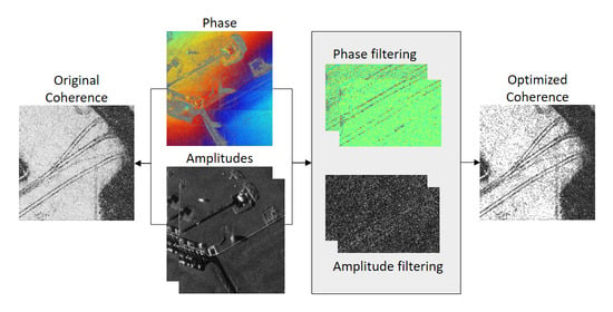
In this paper, a novel algorithm is introduced that aims at enhancing the contrast between high-coherence unchanged areas of the scene and the low-coherence target areas. The algorithm consists of three parts, which are amplitude speckle filtering, removal of the topographic phase and selective noise filtering of the interferometric phase only in high-coherence areas. The novelty of this paper is the careful filtering of the phases and the combination of the different filtering steps, which only when applied together yield the maximum enhancement of the coherence in the high-coherence parts, while leaving the low-coherence parts largely unchanged.

This paper is structured as follows: After the introduction in Section 1, the different schemes to calculate coherence are discussed in Section 2. Section 3 introduces the dataset used for the analysis and the evaluation of the algorithm. Section 4 and Section 5 form the technical heart of this paper, with Section 4 introducing the proposed algorithm, and Section 5 containing the evaluation of the approach on the data set introduced in Section 3. In Section 6, the findings are discussed, and Section 7 contains the conclusion. This paper is an extended version of our paper published at EUSAR 2021 [17].

2. Coherence Calculation

In the literature, several approaches to coherence calculation exist, which all have their own merits and shortcomings. Roughly, these can be categorized into window-based approaches, which estimate coherence in a sliding window of fixed size, and into non-local approaches. Although the window-based approaches are easy to implement and to calculate, the coherence image suffers from artifacts that stem from the rather limited amount of samples used for the calculation. Usually, also a loss of resolution and a blurring of finer structures especially at the edges can be observed. On contrast, non-local approaches come with a higher computational burden, but are able to conserve finer structures in the final output. In a preliminary study to this work [18], the coherence estimator described in [19] was considered. Since this estimator calculates the coherence only using amplitude information, it will not benefit from the contrast enhancement scheme described in Section 4 and thus was not further investigated. Furthermore, in [18], also Non-Local InSAR [20] was used. This estimator, however, takes very long to compute, so it was seen unfit for inclusion in the algorithm below. Instead, a different non-window-based approach (Estimator D below) was added. Thus, four coherence estimators were investigated, which will be introduced briefly in this section.

2.1. Classical Approach, Coherence Estimator A

The classical approach to coherence estimation is given by the following formula:

$$\begin{array}{c}\hfill \gamma \left(x\right):=\frac{{\sum }_{i=1}^N{z}_1\left(i\right)·z_2^{*}\left(i\right)}{\sqrt{\left({\sum }_{i=1}^N{\left|z_1\left(i\right)\right|}^2\right)·\left({\sum }_{i=1}^N{\left|z_2\left(i\right)\right|}^2\right)}},\end{array}$$

(1)

where the calculation is performed in a square sliding window of odd size with N pixels, centered at pixel x. $z_1$ and $z_2$ denote the complex signals of the first and second image, and ${}^{*}$ is complex conjugation. Usually, only the absolute value $\left|\gamma \right|$ is used.

2.2. Coherence Estimator B

One of the problems with Estimator A is, that it is biased if there is topographic phase contained in the interferometric phase. This may lead to wrong estimations of the coherence. This problem is overcome to some extent by the estimator described in [14]. In this paper, first two auxiliary images $w_1$ and $w_2$ are calculated as follows:

$$\begin{array}{ccc}\hfill w_1(m,n)& :=& z_1(m,n)·z_1^{*}(m+1,n)\hfill \end{array}$$

(2)

$$\begin{array}{ccc}\hfill w_2(m,n)& :=& z_2(m,n)·z_2^{*}(m+1,n),\hfill \end{array}$$

(3)

which are estimates of the phase derivative in direction m for the two complex images $z_1$ and $z_2$. Coherence is then calculated in a sliding window using

$$\begin{array}{c}\hfill \gamma \left(x\right):=\frac{{\sum }_{i=1}^N{w}_1\left(i\right)·w_2^{*}\left(i\right)}{\sqrt{\left({\sum }_{i=1}^N{\left|w_1\left(i\right)\right|}^2\right)·\left({\sum }_{i=1}^N{\left|w_2\left(i\right)\right|}^2\right)}},\end{array}$$

(4)

which is the classical formula, except that it is used on the phase derivatives. These calculations can then also be carried out in direction n with analogous formulas. Indeed, in this work, the average of the coherence estimations for directions m and n is used.

2.3. Coherence Estimator C

This estimator was published in [21] and is somewhat simpler and more computationally efficient than the two estimators described in the last two paragraphs. It is also used in a sliding window of fixed size N and is given by the following formula:

$$\begin{array}{c}\hfill \gamma \left(x\right):=\frac{1}{N}·\sum _{i=1}^N\frac{z_1\left(i\right)·z_2^{*}\left(i\right)}{\left|z_1\left(i\right)·z_2^{*}\left(i\right)\right|}.\end{array}$$

(5)

2.4. Coherence Estimator D

Estimator D is an example for a non-window-based estimation scheme. It is based on a multi-stage wavelet transform of the whole interferometric phase image, using only the phase information. This means that the amplitude is completely ignored in this approach, while all of the window-based approaches examined in this paper use both the amplitude and phase information. The algorithm uses two stages of wavelet decomposition and then a final stage of wavelet tree decomposition. In each of these stages, the wavelet coefficients containing a significant amount of signal are identified and enhanced, and at the same time the noisy coefficients are suppressed. The detection of wavelet coefficients containing signal is performed by using the following formula:

$$\begin{array}{c}\hfill {\Gamma }_{sig}=\frac{I_w-2^{2·j^{\prime }}·{\sigma }_v^2}{I_w},\end{array}$$

(6)

where $I_w$ is the intensity of the wavelet coefficients at the highest stage $j^{\prime }=3$, i.e., after the wavelet tree decomposition, and ${\sigma }_v^2$ is the noise power. In [22], a threshold of −1 is suggested to detect those coefficients containing significant signal parts, and all of the wavelet coefficients above the threshold are multiplied by 2. Then, inverse wavelet packet transform is applied. In the remaining two stages, all coefficients detected in one of the previous stages as containing signal are again multiplied by 2. Newly detected signal coefficients at the current stage by Formula (6) are then also multiplied by 2 and added to those coefficients coming from the lower stages. After undoing all of the wavelet transforms, each pixel contains information about the noise-free signal $N_c$, which is linked to the coherence via

$$\begin{array}{c}\hfill N_c=\frac{\pi }{4}\left|\gamma \right|{·}_2{F}_1\left(\frac{1}{2},\frac{1}{2};2;{\left|\gamma \right|}^2\right),\end{array}$$

(7)

where ${}_2{F}_1(a,b;c;z)$ is the Gauss hypergeometric function. From $N_c$, the coherence $\left|\gamma \right|$ can then be inverted using this formula and a look-up table. For details of this algorithm see [22].

2.5. Value Range of the Coherence Estimators

Since the main goal of this paper is to enhance the gray-level difference between the low-coherence changed parts of the scene and the high-coherence surroundings, the value range of these estimators is important. From the formulas of Estimators A–C, it can be easily deduced that the maximum possible value range is the interval [0,1]. For coherence Estimator D, values greater than one can occur, however, following [22], these values are then normalized to [0,1]. A value of one can be obtained if, and only if, all of the contributions are in phase. For Estimators A and B, additionally, a value of one can only be obtained if, and only if, the corresponding amplitudes, respectively, their derivatives (for Estimator B), of the two images within the calculation window are linearly dependent. Considering that in SAR images amplitudes usually are non-zero, coherence can only be zero if the phases of the pixels within the window are such, that the complex numbers cancel out, which is a very special situation. Since coherence is calculated from a finite number of samples, the mean coherence even for completely decorrelated areas is not zero. The minimal mean coherence depends very much on the size of the window for the window-based approaches, and also on the processing of the SAR image itself. For completely uncorrelated speckle, using a $7\times 7$ calculation window, the minimal mean value is about 0.1. This changes quite drastically if, as is the case for the dataset introduced in Section 3, the images are oversampled during the SAR processing. In this case, the speckle is not uncorrelated any more. For the SmartRadar data used in this paper, the oversampling by a factor of 1.4 leads to a theoretical minimal mean coherence of about 0.2. These values were generated by simulating completely decorrelated speckle, then oversampling the image and calculating the mean coherence over a $128\times 128$ pixel image. For stability, this simulation was carried out 100 times and the mean of the coherence means was taken. Thus, even in perfect conditions, the maximal gray-level difference that can be achieved is only about 0.8. This should be kept in mind when interpreting the results presented in Section 5.

3. Dataset

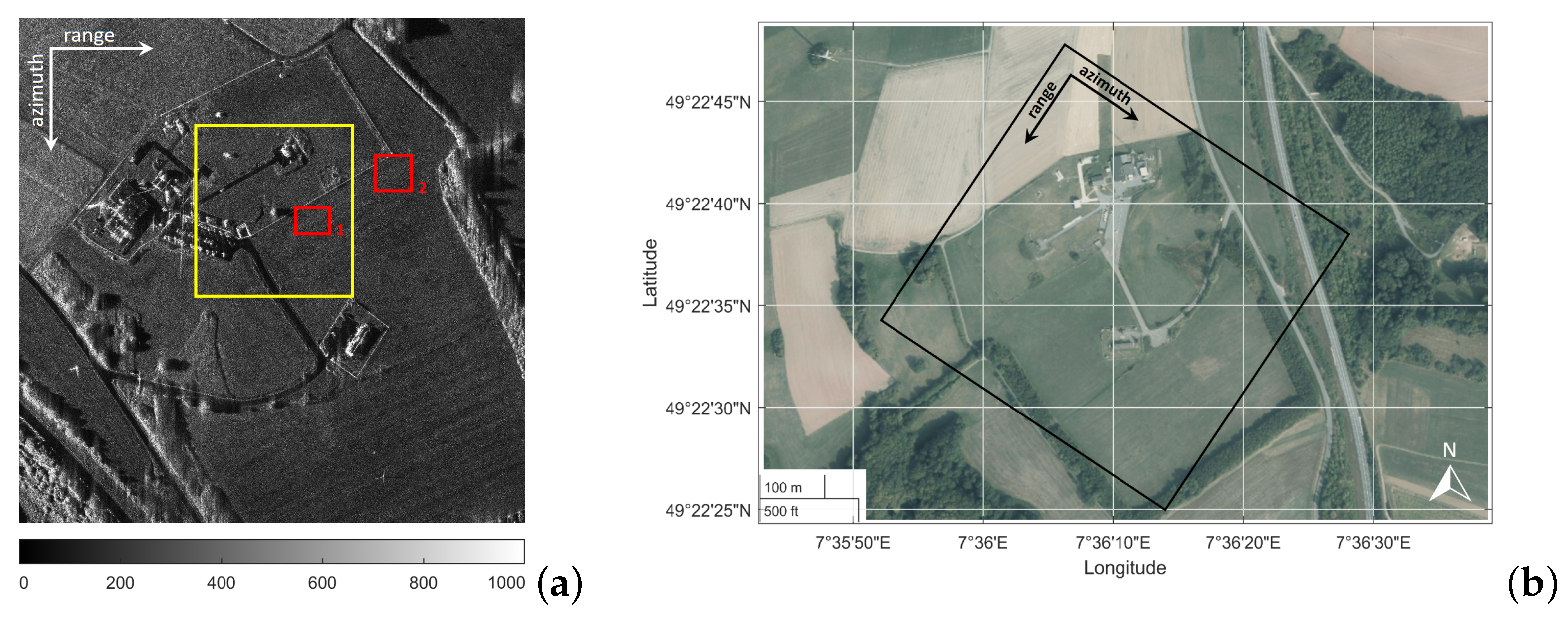
The dataset used in this work was acquired during a measurement campaign at the Bann B installations of POLYGONE Range in western Rhineland-Palatinate, Germany, in 2015. It contains an interferometric image pair that was recorded during two overflights by the airborne SmartRadar sensor operated by Hensoldt Sensors GmbH, mounted on a Learjet. SmartRadar is an X-band sensor with resolution in the decimeter range. The acquisition geometry of the POLYGONE data used in this work can be found in

Table 1. Properties of the POLYGONE acquisitions.

Band	X-band
Resolution	Decimeter range
Slant range distance to first bin	approx. 10,260 m
Flight height above ground	approx. 4270 m
Depression angle first bin	approx. 25${}^{\circ }$
Time between acquisitions	approx. 4 h
Scene center coordinate	49.377036 N, 7.602708 E
(Lat/Lon decimal, WGS84)
Baseline	approx. 32.8 m

.

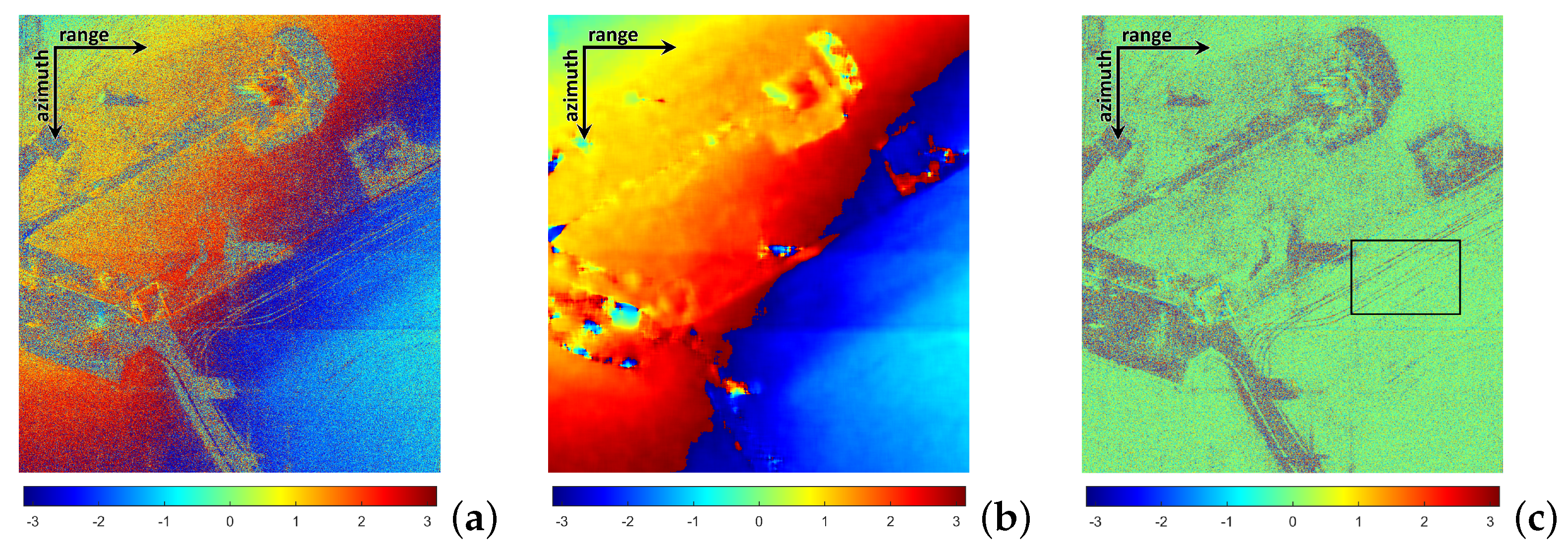
During the data takes, the Learjet operated in autopilot mode, giving very stable and accurate flight paths. Figure 1a shows one of the images recorded during the measurement campaign, while in Figure 1b the area is shown in an optical image. The two areas of interest marked with red boxes will be used in the following sections for the evaluation of the results, while the area marked with the yellow box will be used to show the effect of the removal of the topographic phase.

Note that the SAR image has not been geo-coded nor projected to ground geometry. All of the calculations in the following are performed on the single-look complex images. Furthermore, all of the cut-outs and images derived from the SAR images, unless stated otherwise, have the same azimuth and range direction as the image shown in Figure 1a.

The scene mainly consists of forests and grassland, some roads and the buildings of the Bann B installations of POLYGONE Range. The grassland around the buildings was mowed just one day before the measurement campaign and the mowed, rather tall, grass was left lying on the ground, giving very good coherence in these parts of the image. 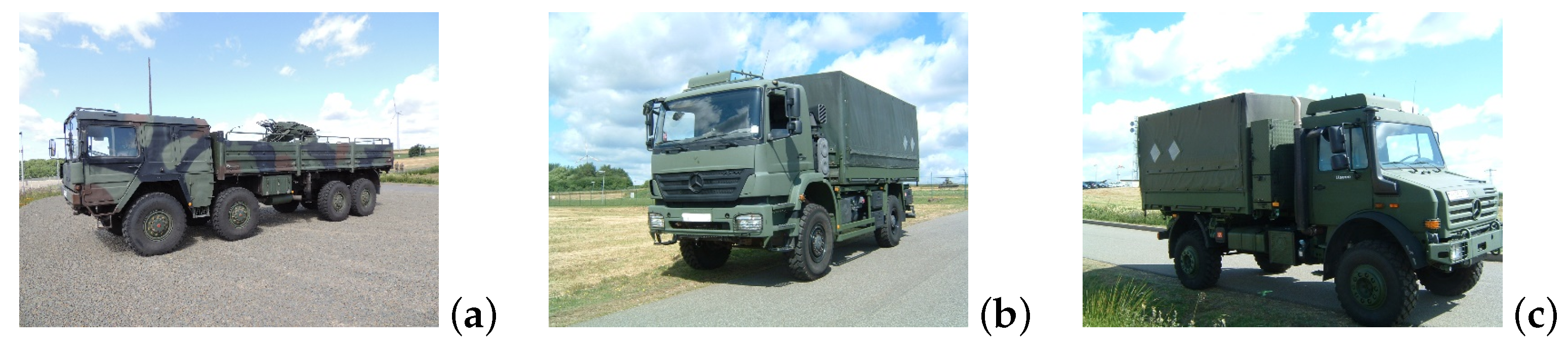The scene was kept as stationary as possible during the SAR image recordings, however, in-between the overflights the three vehicles shown in Figure 2 were driven across the grassland. They moved mainly in straight lines, but at both ends of the tracks, also situations that are more complicated are present, such as curved paths and some intersection of the tracks. We aim at extracting these tracks from the coherence image. To give an idea of the axle and wheel widths of these vehicles, the approximate numbers are given in the following: The MAN 10 to truck has an axle width of 2.2 m and a wheel width of 0.4 m. The axle width of the Mercedes-Benz Axor is about 1.8 m with a wheel width of 0.37 m. The Unimog U5000 has an axle width of 1.92 m and the width of the wheels is about 0.4 m.

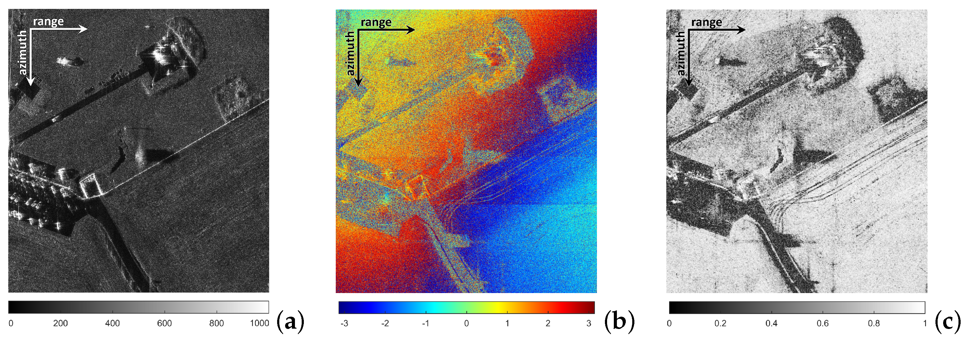
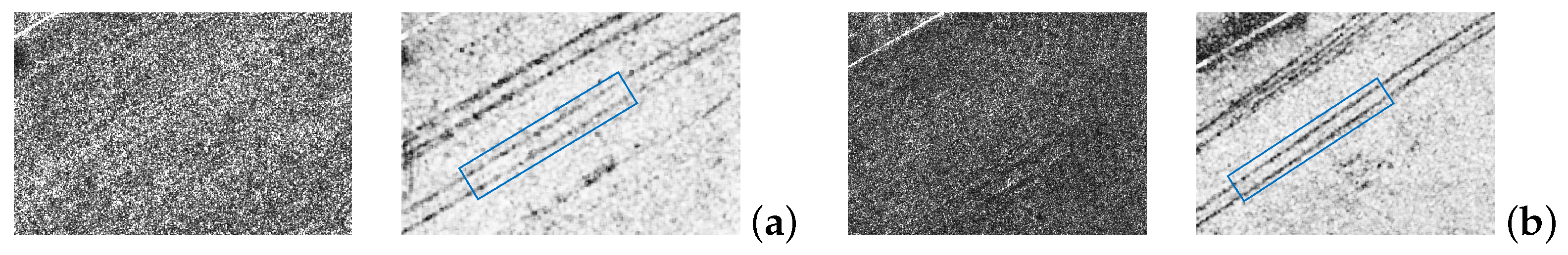
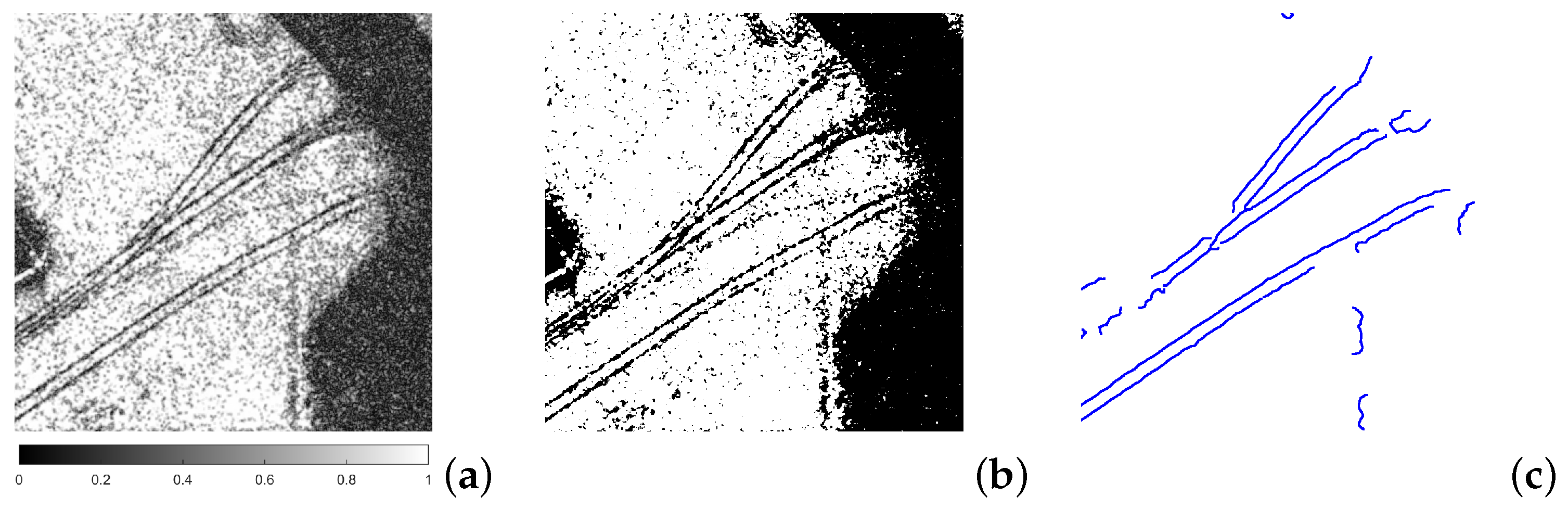
Figure 3 shows a detail of the scene containing a part of the vehicle tracks. In (a) the original amplitude image of the second overflight is shown. Figure 3b contains the interferometric phase, and (c) is the coherence estimate using the classical Estimator A in a $7\times 7$ window. For the choice of this window size, see the discussion in Section 4.1.

Figure 3a shows that the vehicle tracks are not visible in the amplitude image of the second overflight, while they can clearly be seen in both the phase image (b) and the coherence image (c).

4. Coherence Contrast Enhancement

As mentioned in the last section, the goal is to detect the tracks of the vehicles that moved across the grassland at POLYGONE, i.e., a CCD task. Usually, CCD is performed by applying some threshold to the coherence image and then filtering the results. For this to work well, the high-coherence parts of the scene should have good contrast or gray-level difference to the low-coherence (changed) areas.

The ideas for the contrast enhancement come from closely examining Formula (1), the classical formula for coherence estimation. As discussed in Section 2.5, this formula becomes maximal, if the amplitudes of the corresponding pixels within the window are linearly dependent, and are in phase, i.e., the phase difference is zero. 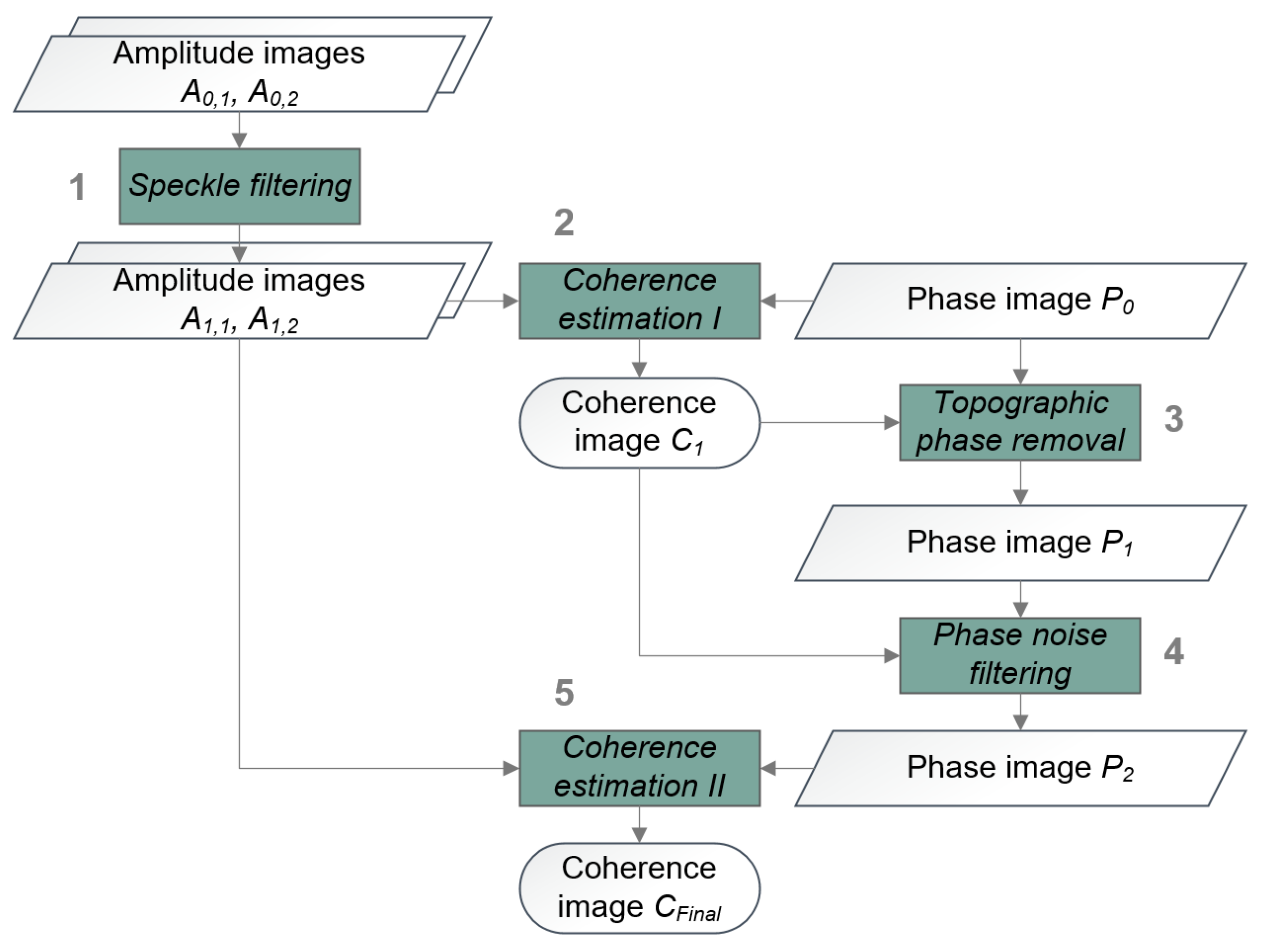So, in order to get as close as possible to such a situation, the following steps are proposed, which are also shown as a flowchart in Figure 4.

1.

Speckle filtering of the amplitudes $A_{0,1}$ and $A_{0,2}$ for the whole image; this leads to the filtered amplitudes $A_{1,1}$ and $A_{1,2}$ being close to constant in small windows;

2.

Calculation of a first coherence estimate $C_1$. There are two possible choices for this step: Using one coherence estimator for the whole algorithm (i.e., the one used in Step 5 below), or using one fixed estimator for this first step, which means that in Step 5 all estimators have the same input. It was decided to conduct two experiments: Experiment 1 uses the filtered amplitudes of Step 1, the classical Estimator A for Step 2 and the estimator of choice for Step 5, while Experiment 2 uses the same coherence estimator for Step 1 and Step 5;

3.

Removal of the topographic phase from the original phase image $P_0$, resulting in the intermediate phase image $P_1$; this leads to the phases being more similar in the high-coherence parts while not changing much in the low-coherence parts; this step uses the coherence estimate of Step 2;

4.

Noise filtering of $P_1$, only in the high-coherence parts, resulting in the phase image $P_2$; this supports the coherence becoming maximal in the high-coherence parts while remaining unchanged in the low-coherence parts. This step also uses the coherence estimate of Step 2;

5.

Re-calculation of the coherence using the coherence estimator of choice, the filtered amplitudes $A_{1,1}$ and $A_{1,2}$ and the filtered phase $P_2$, resulting in the final coherence estimate $C_{Final}$.

Note that Step 1 and Step 3 act on the whole image, thus also altering the values in the low-coherence parts. Indeed, the amplitude filtering in some cases might raise coherence in the low-coherence parts slightly. However, since the interferometric phase in these parts remains random, this effect will not be very pronounced, while in the high-coherence parts, the combined effect of speckle filtering and phase smoothing yields a much higher coherence. As for the topographic phase, if the topography is not very pronounced, in the small windows used for the calculation of the coherence, this amounts to an almost constant factor that is subtracted from all phases within the window, thus only altering the coherence calculation very slightly.

The filtering steps and the methods chosen for the evaluation of the algorithm will be discussed in more detail in the following. We also tried a re-calculation of the coherence after Step 3. However, the differences in the final coherence estimate were minor, while calculation time increased, so this step was dropped in the final algorithm.

4.1. Choice of Window Size

For the window-based approaches of coherence calculation, the size of the calculation window has to be chosen. In this paper, all window-based approaches, except for the removal of the topographic phase, use a $7\times 7$ calculation window. In a previous study [18], the effect of the window size on the coherence estimation was discussed in depth and it was concluded that using a $7\times 7$ estimation window provided the best compromise between stability of statistics and detectability of the rather fine structure of the vehicle tracks. To be consistent with this choice of window size, also the window-based speckle filters, introduced in the next section, were applied with this window size. The non-local SAR speckle filter requires two windows, the comparison window and the search window. For this algorithm, again, the comparison window was set to $7\times 7$ pixels, while the search window was set to $21\times 21$ pixels.

4.2. Speckle Filtering

In the literature, many speckle filters exist, see e.g., [23,24] for overviews of the classical and some more advanced speckle filters, and [25,26] for more recent developments involving convolutional neural networks. Several of these were applied to the original amplitude images $A_{0,1}$ and $A_{0,2}$ to evaluate their impact on the enhancement of the contrast between the high-coherence and the low-coherence parts of the scene. Since the vehicle tracks are not visible in the amplitude images (see Figure 3), the amplitude speckle filtering was applied to the whole image. The investigated speckle filters were

• Lee-Filter ([27]);
• Gamma-MAP ([28]);
• Non-local SAR, non-iterative version ([29]);
• Average filtering.

4.3. Topographic Phase Removal

The first step of phase filtering is the removal of the topographic phase. Figure 3b contains the original interferometric phase $P_0$ for the scene. The figure shows that there is some topography present in the scene, however, this topography is not very pronounced. This is also the assumption for the phase filtering process. The topographic phase is estimated by averaging the interferometric phase in a large ($51\times 51$ pixel) window. Since the phase in the low-coherence parts of the scene contains mainly noise, the phase values are multiplied by the coherence estimate $C_1$ of Step 1, so that the low-coherence pixels contribute less to the average. The effects of this filtering step are shown in Section 5.

4.4. Phase Noise Filtering

The most crucial step in the filtering of the interferometric phases is the suppression of the phase noise. This has to be done very carefully, since the goal is not to smoothen the phases in the low-coherence parts of the scene. The phase smoothing applies a small ($7\times 7$ pixels again) sliding averaging window to the scene. However, only those pixels are filtered, in whose vicinity, i.e., within the filter window area, only a maximum of 11 pixels are below 0.7 in the coherence estimate $C_1$. Since the sliding window is rather small, the vehicle tracks will not be affected by the filtering, while their surroundings will be smoothed. Results of this filtering step on the dataset are shown in Section 5.

4.5. Quantitative Evaluation of Coherence Enhancement

For the evaluation of the improvement of contrast between the high-coherence and low-coherence areas of the scene, two representative parts of the vehicle tracks were chosen. These are marked with red boxes in Figure 1. The main difference between the two areas of interest is that the track in Area 1 is less pronounced than the track in Area 2, meaning it has worse contrast with the coherent surroundings. Figure 5a,b show details of the scene around the areas of interest in the original amplitude image of the second overflight (left), while the corresponding images on the right show the same areas in the coherence image obtained with the original amplitude and phase data and Estimator A. In the coherence images, the actual portion of the tracks used for the qualitative evaluation in Section 5 is marked with a blue rectangle.

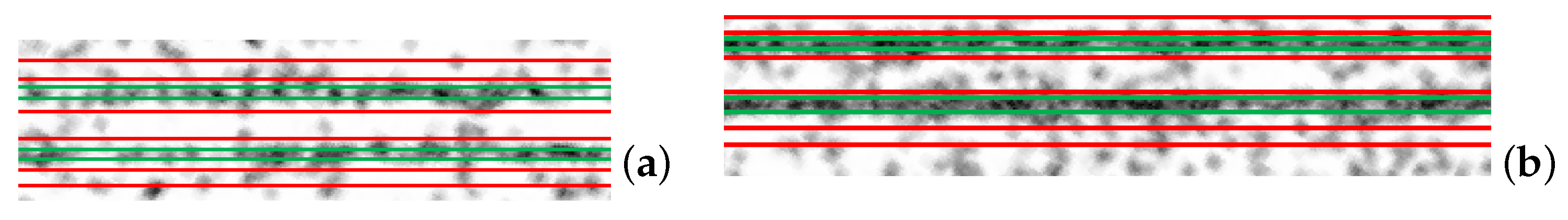
Within these areas, the tracks and their surroundings were manually delineated. To facilitate this, the cutout image parts were rotated so that the tracks were approximately horizontal. The delineation of the areas can be seen in Figure 6. Note the gap between the areas marked as tracks (between the green lines) and those marked as surroundings (between the red lines). These were left on purpose to evaluate the maximal gray-level difference/contrast between the low- and high-coherence areas.

For the evaluation, the average contrast between the areas marked as track (green) and the areas marked as surroundings (red) was calculated. Although contrast is a widely used measure, the raw difference between the gray-levels is considered also very important, especially if a threshold is to be applied to the coherence image. Thus, the average gray-level difference was also calculated.

The contrast $\rho$ is defined as

$$\rho =\frac{{\mu }_C-{\mu }_{IC}}{{\mu }_C+{\mu }_{IC}},$$

(8)

where ${\mu }_C$ and ${\mu }_{IC}$ are the mean gray-values in the high-coherence parts (surroundings) and the low-coherence parts (tracks), respectively.

4.6. Evaluation of the Algorithm with Respect to Detectability of the Tracks

Eventually it is of interest whether the coherence optimization affects the change detection capabilities with regard to the vehicle tracks in the image area. To assess the performance, a track detection was performed on the original coherence, calculated with the original amplitudes and phases, and the optimized coherence $C_{Final}$ using a standard approach, involving an auto-thresholding of the coherence image to obtain a binary image and a subsequent line detection operation. Regarding the auto-thresholding, several standard methods were considered, such as the global entropy method [30] and Otsu’s method [31]. However, results show that not all methods are suitable for the task at hand; in fact, best results were achieved using the mean of coherence values as the threshold. As a standard line detection method, a Steger line operation [32] was then performed on the binarized image (see Section 5.6).

5. Results

In this section, the methods discussed in Section 4 are applied to the Bann B scene and the effects of the filtering are evaluated both visually and quantitatively. Furthermore, the success of the algorithm is demonstrated by extracting the tracks both from the original and from the optimized coherence image, showing that the latter are much more complete than the tracks extracted from the original coherence image.

5.1. Removal of the Topographic Phase

The method to calculate the topographic phase was introduced in Section 4.3. The original interferometric phase is shown in Figure 3b and again in Figure 7a for comparison. The resulting topographic phase, exemplary calculated with the help of the coherence image $C_1$ obtained with Estimator A, can be seen in Figure 7b, and the remaining phase $P_1$ after removal of the topography is shown in Figure 7c. The black rectangle in Figure 7c marks the location of Area 1. This area is used in Figure 8 to demonstrate the effects of the phase noise filtering.

Re-calculation of the coherence after removal of the topographic phase has shown that the impact on the coherence is very small. This was to be expected, since the topography is locally smooth in the area and since the coherence estimation windows are small. The wavelet-based approach (Estimator D), which acts on the whole image at once, basically is a noise filter for the phases. Since the topographic phase is deterministic, this filter also is not affected significantly by the topographic phase.

5.2. Phase Noise Filtering

This is the most crucial step in the algorithm, and the method was introduced in Section 4.4. It is applied to the topography-removed phase shown in Figure 7c. The exemplary coherence estimate used for this step is again the first coherence estimate $C_1$ calculated by Estimator A.

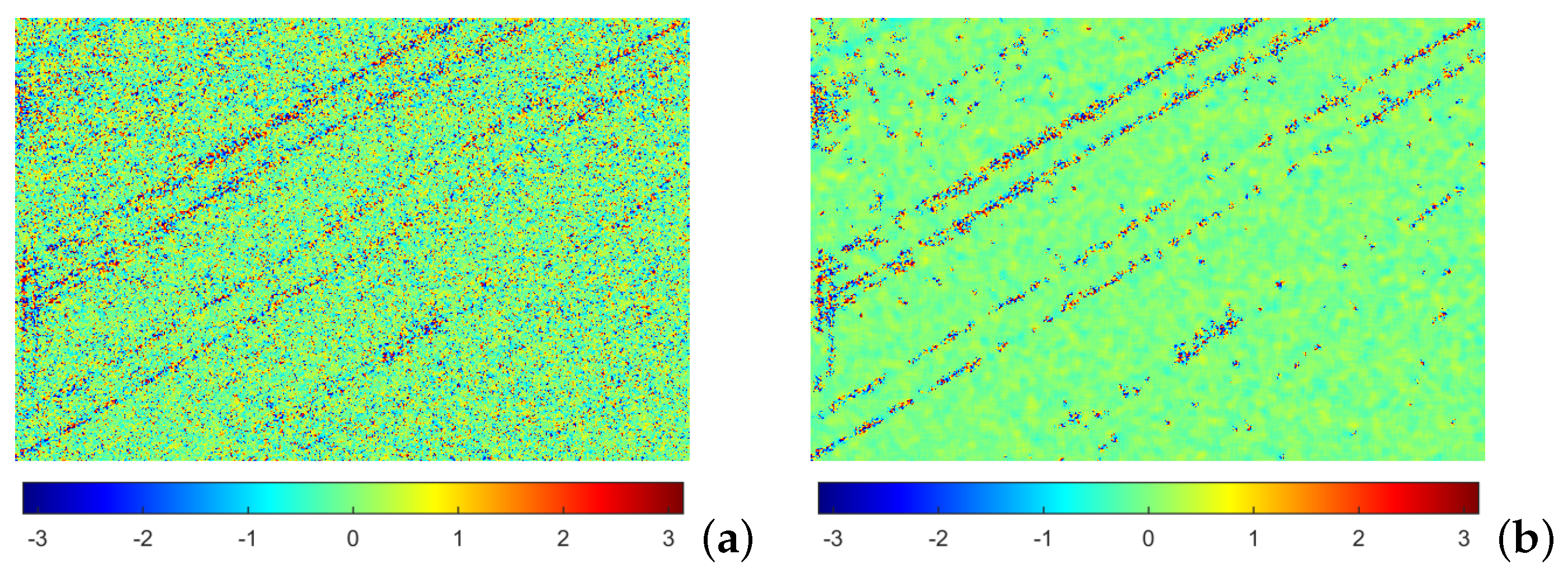
Figure 8a shows a zoom into the part of Figure 7c marked with the black rectangle, which is also Area 1. In Figure 8b, the phase noise in the high-coherence areas is very much suppressed, as was intended, while the low-coherence areas have remained unchanged.

The next two sections contain the quantitative evaluation of the algorithm for the Experiments 1 and 2 described in Section 4, in Areas 1 and 2.

5.3. Quantitative Evaluation, Experiment 1

For Experiment 1, the coherence estimation $C_1$ of Step 2 of the algorithm described in Section 4 was calculated using the classical Estimator A.

Table 2. Average contrast and difference of coherence, Experiment 1, Area 1. L = Lee-Filter [27], GM = GammaMap [28], NL = Non-Local SAR filter, non-iterative version [29], Avg = Multi-look in sliding $7\times 7$ averaging window, TR = Topographic phase removed, NF = Noise-filtered. Best results are highlighted in gray.

Amp.	Phase	A		B		C		D
		Contr.	Diff.	Contr.	Diff.	Contr.	Diff.	Contr.	Diff.
Or.	Or.	0.126	0.195
L	TR + NF	0.132	0.226	0.117	0.198	0.122	0.214	0.126	0.221
GM	TR + NF	0.164	0.271	0.151	0.249	0.163	0.269	0.142	0.240
NL	TR + NF	0.182	0.284	0.176	0.270	0.182	0.284	0.146	0.240
Avg	TR + NF	0.181	0.287	0.176	0.276	0.179	0.286	0.146	0.241

shows the results of Area 1 for the different coherence estimators and the different amplitude filters. Note that even though Estimator D uses only the phase information for the calculation of $C_{Final}$, the different amplitude filters change the coherence image $C_1$ (using Estimator A) slightly. Thus, the filtering steps using $C_1$ also change, which is why the contrast and difference of gray-level for Estimator D are not constant, depending on the amplitude filtering. For comparison with the results of the algorithm, in the first row, the contrast and gray-level difference using Estimator A and the original amplitudes and phases are also shown.

Table 3. Average contrast and difference of coherence, Experiment 1, Area 2. Notation see Table 2.

Amp.	Phase	A		B		C		D
		Contr.	Diff.	Contr.	Diff.	Contr.	Diff.	Contr.	Diff.
Or.	Or.	0.280	0.366
L	TR + NF	0.330	0.469	0.228	0.340	0.317	0.465	0.259	0.399
GM	TR + NF	0.356	0.480	0.257	0.366	0.353	0.479	0.270	0.397
NL	TR + NF	0.358	0.459	0.258	0.342	0.358	0.459	0.270	0.387
Avg	TR + NF	0.361	0.470	0.270	0.364	0.359	0.470	0.271	0.390

contains the corresponding results for Area 2.

As can be seen from the tables, for both areas the average contrast and the average gray-level difference between the unchanged and changed parts of the scene are strongly enhanced.

5.4. Quantitative Evaluation, Experiment 2

For the second experiment, $C_1$ is calculated using the same coherence estimator as for $C_{Final}$. The resulting contrasts and gray-level differences are shown in

Table 4. Average contrast and difference of coherence, Experiment 2, Area 1. Notation see Table 2.

Amp.	Phase	A		B		C		D
		Contr.	Diff.	Contr.	Diff.	Contr.	Diff.	Contr.	Diff.
Or.	Or.	0.126	0.195	0.112	0.171	0.097	0.163	0.123	0.186
L	TR + NF	0.132	0.226	0.109	0.185	0.109	0.194	0.134	0.228
GM	TR + NF	0.164	0.271	0.150	0.235	0.160	0.266	0.134	0.228
NL	TR + NF	0.182	0.284	0.154	0.212	0.181	0.284	0.134	0.228
Avg	TR+NF	0.181	0.287	0.164	0.238	0.177	0.284	0.134	0.228

for Area 1 and in

Table 5. Average contrast and difference of coherence, Experiment 2, Area 2. Notation see Table 2.

Amp.	Phase	A		B		C		D
		Contr.	Diff.	Contr.	Diff.	Contr.	Diff.	Contr.	Diff.
Or.	Or.	0.280	0.366	0.200	0.268	0.237	0.344	0.250	0.326
L	TR + NF	0.330	0.469	0.218	0.324	0.310	0.461	0.258	0.381
GM	TR + NF	0.356	0.480	0.220	0.296	0.352	0.480	0.258	0.381
NL	TR + NF	0.358	0.459	0.195	0.234	0.358	0.459	0.258	0.381
Avg	TR + NF	0.361	0.470	0.212	0.261	0.360	0.471	0.258	0.381

for Area 2. For this experiment, in order to compare the effects of the filtering steps to the original coherences, the coherence for the respective estimator using the original amplitudes and phases are given in the first row of the tables.

5.5. Visual Comparison of Coherence Enhancement

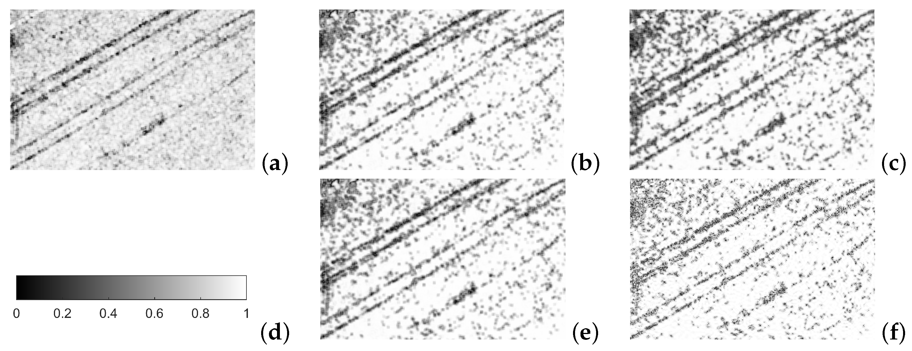
Figure 9 shows the original coherence estimated with Estimator A and the results of Experiment 1 for the different estimators for visual comparison. For this visualization, Area 1 was chosen because it yields the bigger relative improvement in gray-level difference. However, the results for Area 2 are similar. Comparing with the coherence estimated from the original data shown in (a) it can be seen that for all estimators, the examined vehicle track becomes much more pronounced. Note that for direct visual comparison, all images shown in Figure 9 and Figure 10 are scaled between 0 and 1.

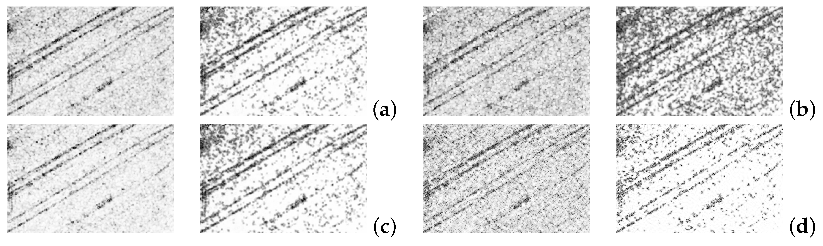
Figure 10 shows the best results for Experiment 2 and Area 1. Since in this experiment the coherence images $C_1$ and $C_{Final}$ are calculated with the same estimator, for each of these the original coherence image, calculated with the original data, is shown (left) along with the best result of the filtering (right).

On average, considering both study areas, the combination of amplitude average filtering (Avg) and the classical coherence estimator A performs best, both when the average contrast and when the average gray-level difference are considered. As for the wavelet-based approach, being the only investigated non-window-based approach, the original paper [22] already mentions that the estimator is biased in low-coherence areas, where it tends to over-estimate coherence, which in this case leads to less contrast.

5.6. Comparison of Track Detection Performance

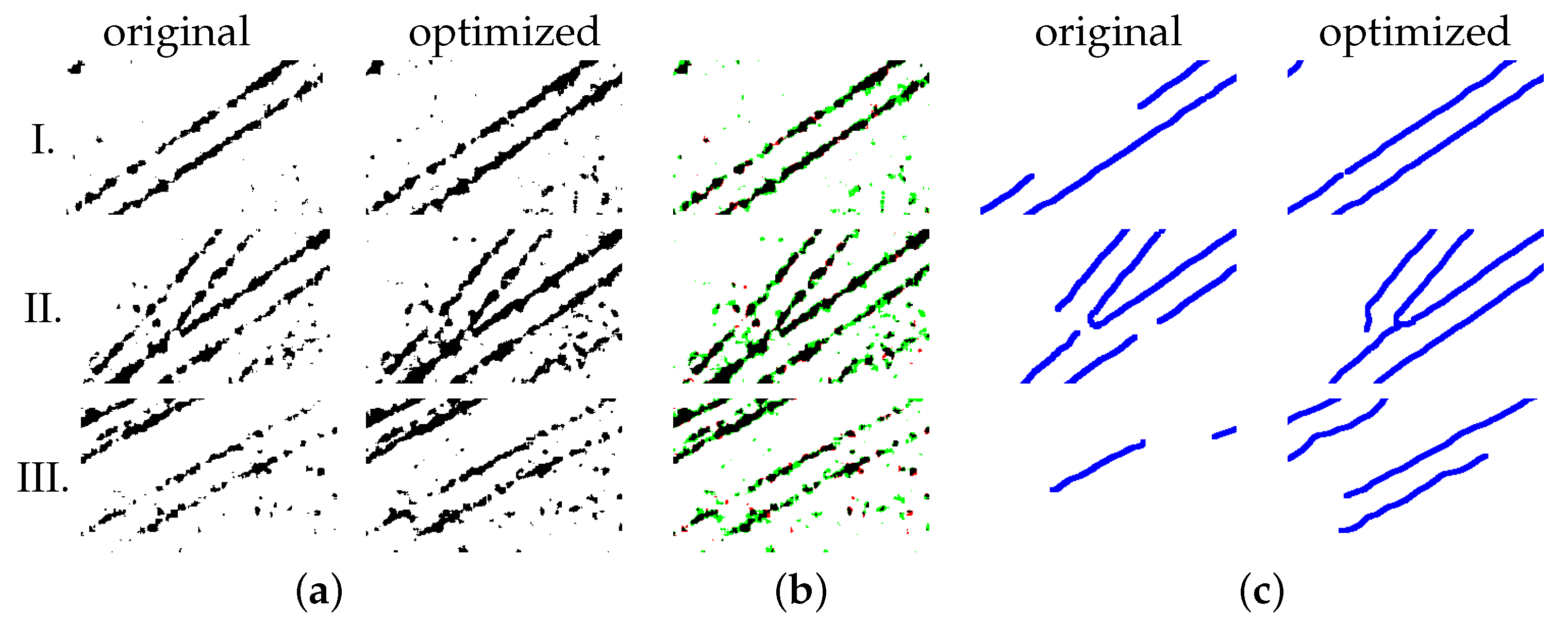
In this section, the success of the coherence contrast enhancement is demonstrated by extracting the tracks both from the original coherence, calculated with original amplitudes and phases, as original image, and from the optimized coherence $C_{Final}$. Since the numerical results, on average over both test areas, showed that average amplitude filtering and the use of Estimator A provided the best enhancement of the coherence, this setup was used for the calculation of $C_{Final}$, and the corresponding original image was also calculated using Estimator A. For better comparison, the test scene was enlarged.

Figure 11 and Figure 12 show the line detection results for the vehicle tracks regarding the original coherence image and the optimized coherence image $C_{Final}$, respectively. It can be observed that the line detection indeed performed better on $C_{Final}$ than on the original image, showing in distinctly fewer discontinuities of the lines. Figure 13 depicts three cutouts of the scene (I.–III.) in more detail, showing the difference on pixel level. The disparity of the binary images is visualized in (b), with green indicating pixel additions, and red indicating pixel omissions. The strengthening of the line structure is perceptible and accordingly the resulting line extractions show distinct improvement.

6. Discussion

Interferometric pairs of SAR images acquired at different times, besides classical amplitude change detection, offer the opportunity to perform CCD, if the time frame between the acquisitions is not too long, or the imaged area, in general, is very stable. While amplitude change detection relies on the change in backscattering coefficients, CCD mainly relies on the properties of the interferometric phase. With this technique, changes can be detected which are not visible or detectable in the amplitude images. Most CCD algorithms rely on a threshold to separate the low-coherence changed areas from the high-coherence unchanged surroundings. For this to work well, the contrast, or gray-level difference between these parts of the image should be as high as possible.

The algorithm introduced in this paper aims at increasing this contrast, by enhancing the coherence in the high-coherence parts of the image and leaving the low-coherence parts largely unchanged. This is achieved by amplitude speckle filtering and a careful noise filtering of the interferometric phase only in areas of high coherence. For speckle filtering, a simple average in a sliding window gave the best results. This might be particular to the situation at hand, where the tracks to be detected are completely located in a rather homogeneous grassland area. However, average filtering is expected to be a good choice in any situation where no subtle structures such as dihedral or trihedral corner reflectors or other textural information need to be preserved. Indeed, one of the quality indices for speckle filters is the mean preservation index (see [24]). In [24], many classical and some advanced speckle filters are investigated, and it is found that at least the classical filters preserve the mean very well, which in turn means that in homogeneous areas they more or less act as an averaging filter.

The choice of window size is to some extent special to the resolution of the data to be processed, and to the size of the structures that should be preserved. However, this parameter can be easily adapted to different situations. For the task at hand, in a preceding study [18] we found that applying a $7\times 7$ window gave the best results for our dataset and the structure of the tracks that are to be detected. The choice of window size then also influences the choice of number of low-coherence points allowed within high-coherence areas to perform phase noise filtering in these areas. This parameter controls which parts of the scene are filtered. The choice of this parameter very much depends on the size and shape of the changes to be detected. For the task of vehicle track detection demonstrated in this paper, the shape of the changed areas is expected to be rather elongated, and to occupy a rather large area of the calculation window. Thus, the value was experimentally set to 11 pixels, which is about 22% of the pixels in the window.

Even though the choices described above are particular to the task at hand and the resolution and temporal baseline of the dataset, we believe that the general algorithm is applicable to a wide range of CCD applications, since it only relies on basic properties of the coherence estimate, which are common to all interferometric image pairs.

The quantitative results obtained with the help of two different areas of the tracks show, that the gray-level difference between the tracks and the coherent surroundings on average could be enhanced by 47% for the weaker track (Area 1) and by 28% for the more pronounced track (Area 2), which already had a good contrast to its surroundings. For Area 2, an average gray-level difference of 0.48 could be reached, which is a very good result, considering that even in perfect conditions, the maximal reachable gray-level difference for the images used in this paper is around 0.8, as demonstrated in Section 2.5.

The assessment of the gray-level enhancement for the detection of the tracks also shows that in comparison with the coherence calculated on the original amplitudes and phases, the lines could be detected much more completely, which demonstrates the success of the presented algorithm for this task.

7. Conclusions

In this paper, an algorithm to enhance the contrast between low-coherence changed parts of a scene and the high-coherence unchanged parts was introduced. This algorithm consists of amplitude speckle filtering, removal of the topographic phase and phase noise filtering, which is only performed in the high-coherence areas. Furthermore, several common speckle filters and several coherence estimators were examined for their suitability for the task of detecting the tracks of several military trucks on a meadow in airborne data with a resolution in the decimeter range. It was concluded that amplitude average filtering in combination with the classical formula for coherence estimation in a $7\times 7$ window gave the best enhancement of contrast for the tracks and their surroundings. Application of an automatic threshold, followed by Steger line extraction showed that the vehicle tracks can be extracted from the optimized coherence much more completely than from the original coherence estimate, showing the success of the method.

Even though the findings are particular to the situation at hand, we believe that the general algorithm will be valuable for other coherent change detection tasks, also using data of different resolutions. Future work could include selective speckle filtering only in the high-coherence areas, which might further enhance the contrast between the changed and unchanged parts of the scene, and the application of the algorithm to data of different resolutions and different tasks to study its performance in these cases. Furthermore, the results of the line extraction will be further processed to suppress false alarms and to fill still existing gaps in the tracks so that ultimately, the tracks will be extracted as completely as possible, to successfully fulfill the coherent change detection task we are aiming at.

References

- Ferretti, A.; Prati, C.; Rocca, F. Permanent scatterers in SAR interferometry. IEEE Trans. Geosc. Remote Sens. 2001, 39, 8–20. [Google Scholar] [CrossRef]
- Zink, M.; Moreira, A.; Bachmann, M.; Rizzoli, P.; Fritz, T.; Hajnsek, I.; Krieger, G.; Wessel, B. The global TanDEM-X DEM—A unique data set. In Proceedings of the 2017 IEEE International Geoscience and Remote Sensing Symposium (IGARSS), Fort Worth, TX, USA, 23–28 July 2017; pp. 906–909. [Google Scholar]
- Lanari, R.; Casu, F.; Manzo, M.; Zeni, G.; Berardino, P.; Manunta, M.; Pepe, A. An Overview of the Small BAseline Subset Algorithm: A DInSAR Technique for Surface Deformation Analysis. In Deformation and Gravity Change: Indicators of Isostasy, Tectonics, Volcanism, and Climate Change; Wolf, D., Fernández, J., Eds.; Birkhäuser: Basel, Switzerland, 2007; pp. 637–661. [Google Scholar]
- Gang, Y. SAR image rapid co-registration based on RD model and coherence interpolation. In Proceedings of the 2011 IEEE International Conference on Spatial Data Mining and Geographical Knowledge Services, Fuzhou, China, 29 June–1 July 2011; pp. 370–372. [Google Scholar]
- Gruber, A.; Wessel, B.; Martone, M.; Roth, A. The TanDEM-X DEM Mosaicking: Fusion of Multiple Acquisitions Using InSAR Quality Parameters. IEEE J. Sel. Top. Appl. Earth Obs. Remote Sens. 2016, 9, 1047–1057. [Google Scholar] [CrossRef]
- Tzouvaras, M.; Danezis, C.; Hadjimitsis, D.G. Small Scale Landslide Detection Using Sentinel-1 Interferometric SAR Coherence. Remote Sens. 2020, 12, 1560. [Google Scholar] [CrossRef]
- Jung, J.; Yun, S.-H. Evaluation of Coherent and Incoherent Landslide Detection Methods Based on Synthetic Aperture Radar for Rapid Response: A Case Study for the 2018 Hokkaido Landslides. Remote Sens. 2020, 12, 265. [Google Scholar] [CrossRef] [Green Version]
- Washaya, P.; Balz, T.; Mohamadi, B. Coherence Change-Detection with Sentinel-1 for Natural and Anthropogenic Disaster Monitoring in Urban Areas. Remote Sens. 2018, 10, 1026. [Google Scholar] [CrossRef] [Green Version]
- Stephenson, O.L.; Kohne, T.; Zhan, E.; Cahill, B.E.; Yun, S.-H.; Ross, Z.E.; Simons, M. Deep Learning-Based Damage Mapping With InSAR Coherence Time Series. IEEE Trans. Geosc. Remote Sens. 2021, 1–17. [Google Scholar] [CrossRef]
- Havivi, S.; Amir, D.; Schvartzman, I.; August, Y.; Maman, S.; Rotman, S.R.; Blumberg, D.G. Mapping dune dynamics by InSAR coherence. Earth Surf. Process. Landforms 2018, 43, 1229–1240. [Google Scholar] [CrossRef]
- Cigna, F.; Tapete, D. Tracking Human-Induced Landscape Disturbance at the Nasca Lines UNESCO World Heritage Site in Peru with COSMO-SkyMed InSAR. Remote Sens. 2018, 10, 572. [Google Scholar] [CrossRef] [Green Version]
- Malinas, R.; Quach, T.; Koch, M.W. Vehicle track detection in CCD imagery via conditional random field. In Proceedings of the 49th Asilomar Conference on Signals, Systems and Computers, Pacific Grove, CA, USA, 8–11 November 2015; pp. 1571–1575. [Google Scholar]
- Wang, Z.; Wang, Y.; Wang, B.; Hu, X.; Song, C.; Xiang, M. Human Activity Detection Based on Multipass Airborne InSAR Coherence Matrix. IEEE Geosc. Remote Sens. Lett. 2021, 1–5. [Google Scholar] [CrossRef]
- Sosnovsky, A.; Kobernichenko, V. Algorithm of Interferometric Coherence Estimation for Synthetic Aperture Radar Image Pair. In Proceedings of the 4th International Conference on Analysis of Images, Social Networks and Texts (AIST), Yekaterinburg, Russia, 9–11 April 2015. [Google Scholar]
- Wahl, D.E.; Yocky, D.A.; Jakowatz, C.V.; Simonson, K.M. A New Maximum-Likelihood Change Estimator for Two-Pass SAR Coherent Change Detection. IEEE Trans. Geosc. Remote Sens. 2016, 54, 2460–2469. [Google Scholar] [CrossRef]
- Sabry, R. Improving SAR-Based Coherent Change Detection Products by Using an Alternate Coherency Formalism. IEEE Geosci. Remote Sens. Lett. 2021, 18, 1054–1058. [Google Scholar] [CrossRef]
- Hammer, H.; Lorenz, F.; Cadario, E.; Kuny, S.; Thiele, A. Enhancement of Coherence Images for Coherent Change Detection. In Proceedings of the European Conference on Synthetic Aperture Radar (EUSAR 2021), Virtual, 29 March–1 April 2021; pp. 881–886. [Google Scholar]
- Hammer, H.; Thiele, A.; Lorenz, F.; Cadario, E.; Kuny, S.; Schulz, K. A Comparative Study of Coherence Estimators for Interferometric SAR Image Co-Registration and Coherent Change Detection. In Proceedings of the SPIE, Image and Signal Processing for Remote Sensing XXV, Strasbourg, France, 9–11 September 2019; Volume 11155, pp. 1115511-1–1115511-12. [Google Scholar]
- Gatelli, G.; Monti-Guarnieri, A.; Prati, C. Coherence Estimation of Interferometric SAR Images. In Proceedings of the 1996 8th European Signal Processing Conference (EUSIPCO 1996), Trieste, Italy, 10–13 September 1996. [Google Scholar]
- Deledalle, C.-A.; Denis, F.; Tupin, F. NL-InSAR: Non-Local Interferogram Estimation. IEEE Trans. Geosc. Remote Sens. 2011, 49, 1441–1452. [Google Scholar] [CrossRef]
- Mu, D.; Lai, C.; Lin, Y. Modifying of the Coherence Estimator for Interferometric SAR. In Proceedings of the 1st Asian and Pacific Conference on Synthetic Aperture Radar (APSAR2007), Huangshan, China, 5–9 November 2007; pp. 2661–2672. [Google Scholar]
- Lopez-Martínez, C. Multidimensional Speckle Noise, Modeling and Filtering Related to SAR Data. Ph.D. Thesis, Universitat Politècnica de Catalunya, Barcelona, Spain, 2 June 2003. [Google Scholar]
- Banerjee, S.; Sinha Chaudhuri, S. A Review on various Speckle Filters used for despeckling SAR images. In Proceedings of the Second International Conference on Computing Methodologies and Communication (ICCMC), Erode, India, 15–16 February 2018; pp. 68–73. [Google Scholar]
- Misra, A.; Ajmera, D. Analysis of Adaptive and Advanced Speckle Filters on SAR Data. IOSR J. Comput. Eng. 2017, 19, 48–54. [Google Scholar] [CrossRef]
- Cozzolino, D.; Verdoliva, L.; Scarpa, G.; Poggi, G. Nonlocal CNN SAR Image Despeckling. Remote Sens. 2020, 12, 1006. [Google Scholar] [CrossRef] [Green Version]
- Zhang, Q.; Yuan, Q.; Li, J.; Yang, Z.; Ma, X.; Shen, H.; Zhang, L. Learning a Dilated Residual Network for SAR Image Despeckling. Remote Sens. 2018, 10, 196. [Google Scholar] [CrossRef] [Green Version]
- Lee, J.-S. Digital Image Enhancement and Noise Filtering by Use of Local Statistics. IEEE Trans. Pattern Anal. Mach. Intell. 1980, PAMI-2, 165–168. [Google Scholar] [CrossRef] [PubMed] [Green Version]
- Lopes, A.; Nezry, E.; Touzi, R.; Laur, H. Structure Detection and Statistical Adaptive Speckle Filtering in SAR Images. Intern. J. Remote Sens. 1993, 14, 1735–1758. [Google Scholar] [CrossRef]
- Deledalle, C.-A.; Denis, L.; Tupin, F.; Reigber, A.; Jäger, M. NL-SAR: A Unified Non-Local Framework for Resolution-Preserving (Pol)(In)SAR Denoising. IEEE Trans. Geosc. Remote Sens. 2015, 53, 2021–2038. [Google Scholar] [CrossRef] [Green Version]
- Kapur, J.N.; Sahoo, P.K.; Wong, A.K.C. A New Method for Gray-Level Picture Thresholding Using the Entropy of the Histogram. Comput. Vis. Graph. Image Process. 1985, 29, 273–285. [Google Scholar] [CrossRef]
- Otsu, N. A threshold selection method from gray-level histograms. IEEE Trans. Syst. Man Cyber. 1979, 9, 62–66. [Google Scholar] [CrossRef] [Green Version]
- Steger, C. An unbiased detector of curvilinear structures. IEEE Trans. Pattern Anal. Mach. Intell. 1998, 20, 113–125. [Google Scholar] [CrossRef] [Green Version]
Figure 1.
(a) SmartRadar image of the POLYGONE scene, areas of interest marked with red boxes; the yellow box marks the area used in the following sections; (b) Optical image of the area, the area contained in the SAR image is marked with a black box. Optical image DOP40 ©GeoBasis-DE/LVermGeoRP 2021.
Figure 2.
Vehicles moved across the grassland. (a) MAN 10 to truck; (b) Mercedes-Benz Axor truck; (c) Unimog U5000 truck.
Figure 3.
Detail of POLYGONE scene. (a) Original amplitude image of second overflight; (b) Interferometric phase; (c) Coherence.
Figure 4.
Flowchart showing the five steps of the proposed optimization process.
Figure 5.
Areas of interest. (
a) Area 1; (
b) Area 2; Left: Original amplitude image; Right: Coherence estimate with original data and Estimator A. The amplitude images have the same scaling as
Figure 3a, and the coherence images have the same scaling as
Figure 3c.
Figure 6.
Vehicle tracks used for quantitative evaluation. (a) Area 1; (b) Area 2. Track areas are between green lines, surroundings between red lines. For the extraction the tracks were rotated, so that the image orientation for these two images is not conformal with the rest of the images.
Figure 7.
Removal of the topographic phase. (a) Original phase image ; (b) Estimated topographic phase; (c) Residual phase after topography removal. The black rectangle in (c) marks Area 1.
Figure 8.
Effect of phase filtering. (a) Topography-removed phase ; (b) Topography-removed and noise filtered phase .
Figure 9.
Results of Experiment 1, Area 1. (a) Coherence estimate of Estimator A with original amplitudes and phases; Best results with respect to gray-level difference using Estimator A for and (b) Estimator A; (c) Estimator B; (e) Estimator C; (f) Estimator D for ; (d) Common scaling for all images in the figure.
Figure 10.
Results of Experiment 2, Area 1. Original coherence with original amplitudes and phases (
left),
(
right) for (
a) Estimator A; (
b) Estimator B; (
c) Estimator C; (
d) Estimator D. The scaling is the same as in
Figure 11.
Results of track detection on the original image. (a) Coherence image; (b) Binary image after auto-thresholding; (c) Extracted Steger lines.
Figure 12.
Results of track detection on . (a) Coherence image; (b) Binary image after auto-thresholding; (c) Extracted Steger lines.
Figure 13.
Impact of coherence optimization on auto-thresholding and line detection for three details (I.–III.) of the scene. (a) Binary image for original and optimized coherence; (b) Difference of the binary images (green: additions, red: omissions); (c) Line extractions for original and optimized coherence.