A Robust Hybrid Deep Learning Model for Spatiotemporal Image Fusion

Abstract

Dense time-series remote sensing data with detailed spatial information are highly desired for the monitoring of dynamic earth systems. Due to the sensor tradeoff, most remote sensing systems cannot provide images with both high spatial and temporal resolutions. Spatiotemporal image fusion models provide a feasible solution to generate such a type of satellite imagery, yet existing fusion methods are limited in predicting rapid and/or transient phenological changes. Additionally, a systematic approach to assessing and understanding how varying levels of temporal phenological changes affect fusion results is lacking in spatiotemporal fusion research. The objective of this study is to develop an innovative hybrid deep learning model that can effectively and robustly fuse the satellite imagery of various spatial and temporal resolutions. The proposed model integrates two types of network models: super-resolution convolutional neural network (SRCNN) and long short-term memory (LSTM). SRCNN can enhance the coarse images by restoring degraded spatial details, while LSTM can learn and extract the temporal changing patterns from the time-series images. To systematically assess the effects of varying levels of phenological changes, we identify image phenological transition dates and design three temporal phenological change scenarios representing rapid, moderate, and minimal phenological changes. The hybrid deep learning model, alongside three benchmark fusion models, is assessed in different scenarios of phenological changes. Results indicate the hybrid deep learning model yields significantly better results when rapid or moderate phenological changes are present. It holds great potential in generating high-quality time-series datasets of both high spatial and temporal resolutions, which can further benefit terrestrial system dynamic studies. The innovative approach to understanding phenological changes’ effect will help us better comprehend the strengths and weaknesses of current and future fusion models.

1. Introduction

Monitoring rapid temporal changes at high spatial resolutions has been increasingly demanded in remote sensing studies for a better understanding of dynamic systems (e.g., terrestrial ecosystems and urban systems) [1]. Specifically, for agricultural applications, capturing rapid phenological changes at the field level is highly desired, as it provides valuable information of the crops grown in individual farm fields [2]. Such phenological information can contribute to improving crop mapping, crop yield estimation, crop progress, and condition monitoring [2,3,4,5,6,7]. Time-series field-level crop information is needed for more precise and timely agricultural monitoring and agronomic managements [8]. Similar demands for time-series information at high spatial resolutions also exist in studies of natural disturbances and urban systems [9,10]. Despite the continuingly increasing amount of satellites in recent years, most satellites still cannot provide imagery with both high spatial and temporal resolutions due to the sensor tradeoff. To fully take advantage of the current collection of remote sensing datasets, fusing the satellite imagery of different spatial and temporal resolutions becomes indispensably necessary. Spatiotemporal image fusion provides a feasible solution to synthesize multi-source remote sensing images and to generate the fused imagery with both high spatial and temporal resolutions.

Spatiotemporal image fusion has been studied and utilized for blending multi-source satellite remote sensing images, typically with image pairs consisting of high-spatial-low-temporal-resolution images (a.k.a. fine images, such as Landsat) and high-temporal-low-spatial-resolution images (a.k.a. coarse images, such as MODIS) that are acquired on the same dates [11]. It attempts to predict the fine image of the desired date using the coarse image on the prediction date and one or two image pairs of surrounding dates. Currently existing spatiotemporal fusion methods can be classified into the following categories: weight function-based, unmixing-based, Bayesian-based, learning-based, and integrated methods [1]. To date, weight function-based methods have been the most widely used spatiotemporal fusion methods. Weight function-based methods predict reflectance of fine pixels by information from neighboring coarse pixels integrated by a weight function. Pixels with lower spectral difference, temporal difference, and spatial distance are normally assigned with larger weights [1,12]. Unmixing-based methods use the linear spectral unmixing framework to predict the reflectance of fine pixels. Unmixing-based methods usually define the endmembers based on the fine images, and unmix the coarse image with defined endmembers in a moving window to predict corresponding fine image spectral reflectances [13]. Further improvements include modifying moving window sizes, preventing drastically different reflectances of endmembers, and refining the process of defining endmembers [5,14,15]. Bayesian-based methods consider the fusion process as the maximum a posterior probability (MAP) estimation of the to-be-predicted image. The predicted image is obtained through maximizing the conditional probability given the existing fine and coarse images [16,17,18,19]. Learning-based methods utilize machine learning, and, more recently, deep learning techniques to model the spatiotemporal relationships between the existing coarse and fine images for spectral estimation of the to-be-predicted fine image [20,21,22]. Integrated methods hybridize two or more of the aforementioned approaches to leverage the strengths of different spatiotemporal fusion methods and to provide more accurate fusion results [23]. While the abovementioned methods have been successfully employed to fuse images with different spatial and temporal resolutions, they may have limited capabilities in predicting rapid temporal phenological changes among the imagery [10,12,24,25]. The methods’ performance may degrade when the temporal phenological changes are rapid and non-linear as most of them assume linear temporal changes among the imagery.

Deep learning is regarded as a breakthrough and has been successfully applied in many fields including remote sensing [26,27,28]. Deep learning can exploit multiple levels of feature representations from the data with minimal prior knowledge required [29]. It embodies a multitude of advanced modeling architectures to learn knowledge from large amounts of complex data. Commonly used deep learning modeling architectures include convolutional neural network (CNN), autoencoder (AE), recurrent neural network (RNN), and generative adversarial networks (GAN) [27]. So far, the most widely used model in remote sensing is CNN [26,27]. With its convolution operation, CNN can automatically extract spatial and textural feature representations from images, which are particularly beneficial in image classification and object detection [30,31]. The convolution operation of CNN is also invariant to translations of spatial features and is computationally efficient. AE can discover efficient representations and structures of the data and has been used in remote sensing for feature learning. RNN is utilized for modeling the temporal pattern or dependence of sequential data. In remote sensing, RNN has been used to learn the temporal features in time-series data for disturbance detection, crop classification, etc. Long short-term memory (LSTM) is a variation of RNN and can more effectively learn temporal patterns over a long time period [32,33,34].

Recent advances in deep learning provide new opportunities to model the complex temporal dynamic changes among the imagery, as well as capture the spatial relationships in spatiotemporal image fusion. For instance, the model of spatiotemporal fusion using deep convolutional neural networks (STFDCNN) demonstrates the potential of multi-layer CNN in image fusion, particularly in image spatial super-resolution to recover the degraded details from the coarse images [22]. A two-stream CNN fusion model, named StfNet, is proposed to better leverage the textural information in the two neighboring fine images for the spatiotemporal fusion, instead of solely restoring the texture from the coarse images. The two-stream architecture also enables the consideration of the temporal information between the fine images [35]. The spatiotemporal fusion method using a GAN (STFGAN) utilizes a GAN model with a residual-block architecture to effectively model the relationship between fine and coarse images, especially for capturing more textural details [36]. By learning the spatial or temporal feature representations, those deep learning modeling architectures hold large potentials to advance the spatiotemporal image fusion. However, most of those deep learning-based models are not designed for characterizing rapid or non-linear phenological changes. The temporal dependence between the prediction date and the acquisition dates of available images is not explicitly modeled by current models. Thus, a more appropriate deep learning modeling structure is to be explored to retrieve both the spatial relationship between the coarse and fine images, as well as the temporal changing pattern from the images acquired on different dates.

Apart from a more appropriate modeling design for spatiotemporal fusion, it is critical to systematically assess the performance of spatiotemporal fusion models, especially how the models are influenced by varying levels of temporal phenological changes of the imagery. As satellite images are subject to cloud contamination and atmospheric interferences, the number of images suitable for spatiotemporal fusion varies across years and locations. The image pairs acquired on different dates may maintain comparable spectral characteristics (e.g., minimum phenological change) or dramatically different ones (e.g., rapid phenological change). The predicted image may also exhibit different levels of changes compared to the image pairs. This diverse range of temporal phenological changes among the dates may subsequently affect the performance of spatiotemporal fusion models. For example, crop species in agricultural systems may undergo drastic phenological changes during relatively short growing periods. The multi-date images for spatiotemporal fusion may possess dramatic changing characteristics. However, it is still not clear how the extent of crop phenological changes documented on multi-date images affects the spatiotemporal fusion results [1]. A comprehensive and systematic scenario design is, thus, desired to evaluate how fusion models perform under various temporal changing circumstances. Such an evaluation can shed light on the strengths and weaknesses of different fusion models and be instructional for the fusion model selection and improvement.

The objective of this study is to develop a novel hybrid deep learning-based spatiotemporal image fusion model that can robustly predict a range of temporal phenological changes in dynamic systems. Specifically, we seek to: (1) devise a hybrid deep learning-based modeling architecture for spatiotemporal image fusion through integrating super-resolution CNN (SRCNN) and LSTM; (2) design various temporal phenological change scenarios among the fusion imagery to systematically evaluate the performance robustness of the image fusion model; and (3) conduct a comprehensive comparison among our hybrid model and three benchmark fusion models. By integrating SRCNN and LSTM, the devised hybrid deep learning model employs an innovative model structure to directly model the temporal dependence and the spatial relationship among images, and to advance the model ability to robustly predict rapid non-linear phenological changes. The MODIS and Landsat images are used as coarse and fine images, respectively.

2. Materials and Methods

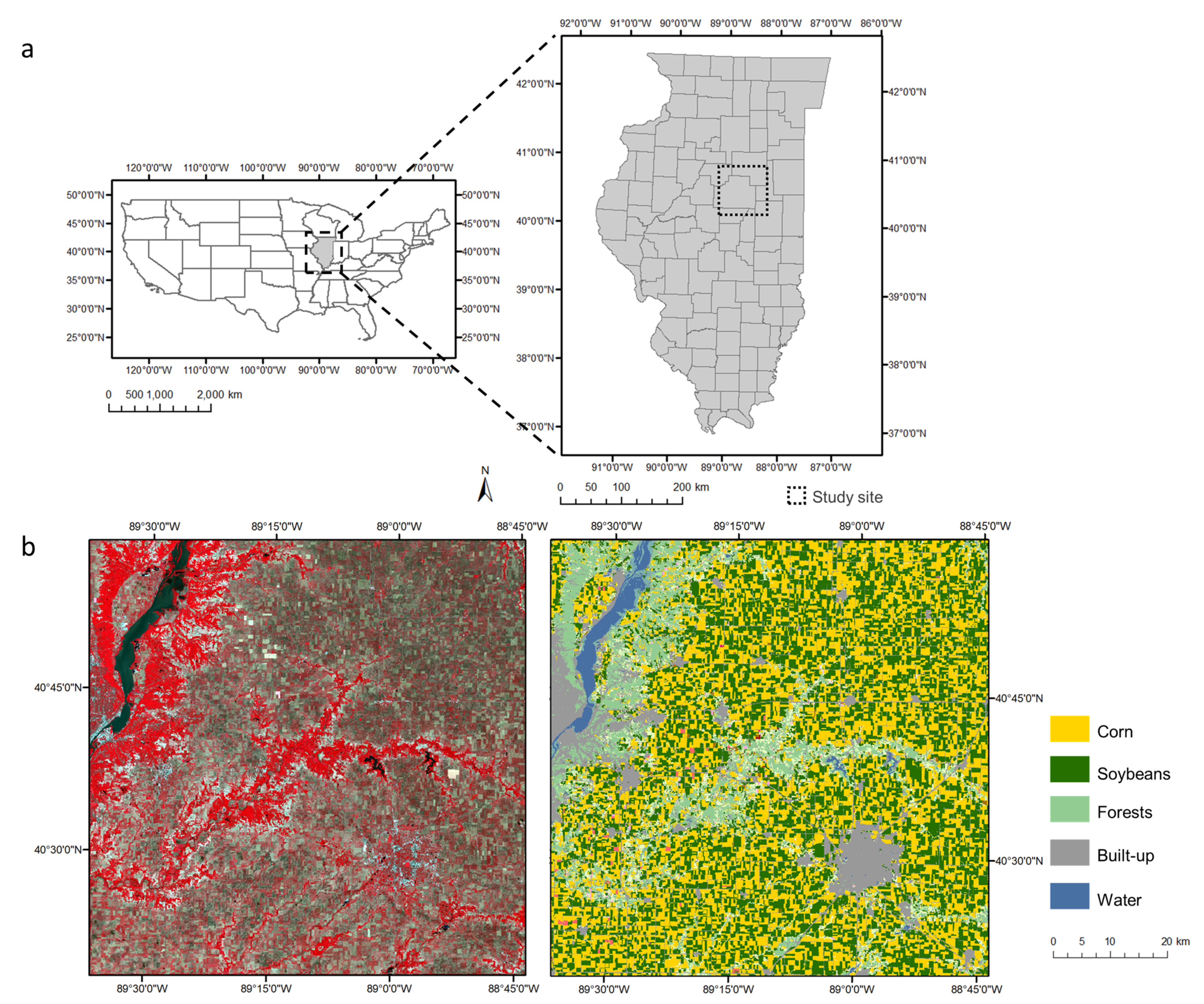
2.1. Study Area

The study site is near Champaign County, located in central Illinois, US (Figure 1). Illinois is an important agricultural producing state in the US. Corn and soybeans are the two main crop types grown in the study site, taking up 37% and 35% of the area, respectively [37]. The study site also contains other land cover classes including forests, built-up areas, and water bodies (Table S1). Central Illinois is selected for our experiments because (1) the crops are the main source of phenological change in the study site and undergo fast phenological changes in growing seasons; and (2) the sizes of crop fields are much smaller than the size of a MODIS pixel (500 m), which makes spatiotemporal fusion desirable to obtain field-level information.

2.2. Satellite Data

In this study, we use MODIS MCD43A4 nadir BRDF-adjusted surface reflectance (NBAR) products (H11V04) as coarse images and Landsat-8 OLI level-2 surface reflectance products (row: 023, path: 032) as fine images. The MODIS MCD43A4 products are temporally dense with daily observations but have a relatively coarse spatial resolution of 500 m. The Landsat data have a finer spatial resolution of 30 m with a 16-day revisit cycle. Six cloud-free Landsat images in 2017 are used in this study. The MODIS images acquired on those dates are collected accordingly to formulate the MODIS-Landsat image pairs. The MODIS and Landsat images are geospatially co-registered before they are used for image fusion [11]. The MODIS images are also resampled to 30-m resolution using bilinear interpolation. The six dates of the MODIS-Landsat image pairs are 11 June, 27 June, 29 July, 15 September, 17 October, and 20 December (day of year [DOY]: 162, 178, 210, 258, 290, and 354). Six shared bands of the MODIS and Landsat data are utilized for spatiotemporal image fusion, namely blue, green, red, near-infrared (NIR), short-wave infrared 1 (SWIR1), and SWIR2 bands.

2.3. Simulation Data

The satellite data, especially the Landsat images, are not always readily available due to the relatively long revisit cycle and cloud cover. To facilitate a more comprehensive understanding of how the fusion models perform at varying image acquisition dates, we generate a simulation dataset of MODIS-Landsat image pairs for the whole year of 2017 using the daily MODIS images and Cropland Data Layer (CDL). The CDL data are produced by the National Agricultural Statistics Service of United States Department of Agriculture (USDA NASS) at a spatial resolution of 30 m [38]. They have been widely utilized as the reference data to understand the geographic distributions of crop species (e.g., corn and soybeans), as well as other major land covers (e.g., built-up, water, and forests). Time-series mean spectral reflectances of the major land covers in the main study site are generated through the whole-year MODIS imagery in combination with the CDL, and those obtained mean spectral reflectance values are assigned to the pixels in the CDL based on their land cover types to generate the simulated MODIS-Landsat image pairs. The specific process of generating the simulation dataset is described in Section S1 of the Supplementary Material and presented in Figure S1.

The simulated images contain six bands: blue, green, red, NIR, SWIR1, and SWIR2. The simulation dataset mimics temporal phenological change patterns in reflectance and the spatial configurations of five major land cover classes: corn, soybeans, forests, built-up areas, and water bodies (Figure S2). While satellite image pairs cannot have consecutive full-year coverage, the simulation dataset provides more flexibility in examining the effects of varying levels of phenological changes on the fusion results.

2.4. Additional Test Sites

Apart from the main study site in central Illinois, three additional study sites across the U.S. are selected to evaluate the generalization ability of the proposed hybrid deep learning model using the real satellite data. The three additional sites are namely the Oklahoma site (located in Northern Oklahoma, including the counties of Grant, Kay, etc.), the Chicago site (including Chicago metropolitan area in Illinois), and the Harvard Forest site in Massachusetts (Figure S3). The three additional test sites are representative of agricultural area with diverse crop types, urban area, and forest area, respectively. The Oklahoma site is an agricultural area where the crops are grown more diversely compared to the main study site, including winter wheat, soybeans, double cropping of winter wheat and soybeans, sorghum, cotton, etc. (Table S2). The diverse collection of crop types gives the Oklahoma site more complex phenological changing patterns as well as a more heterogeneous landscape. The Chicago site mainly consists of built-up areas (Table S3). The urban landscapes in Chicago are heterogeneous with a mixture of various sizes of buildings, roads, parks, and urban vegetation. The phenological temporal changes are predominantly caused by urban vegetation in this area. The Harvard Forest site mainly consists of forests (Table S4), with a relatively homogenous landscape.

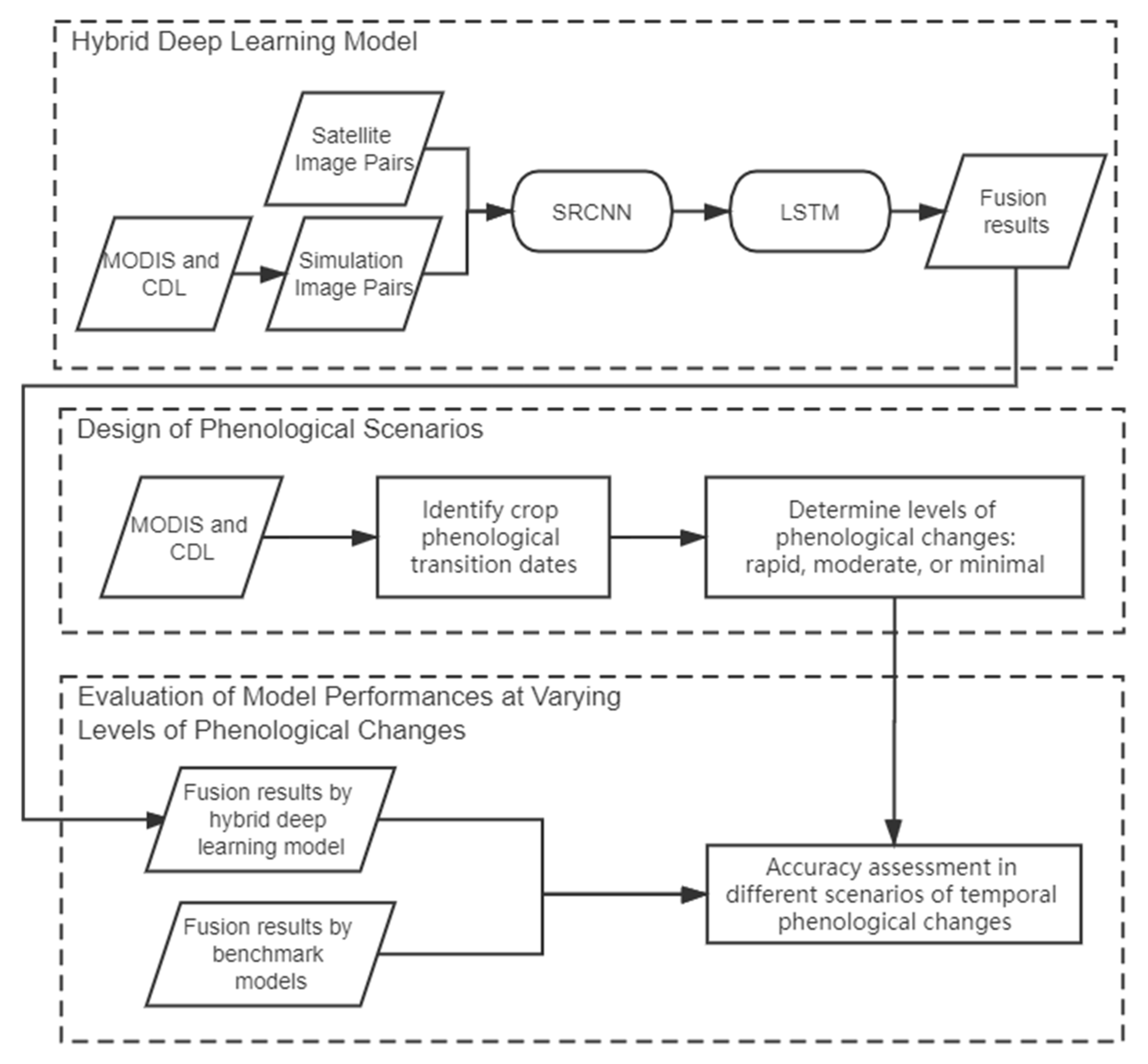
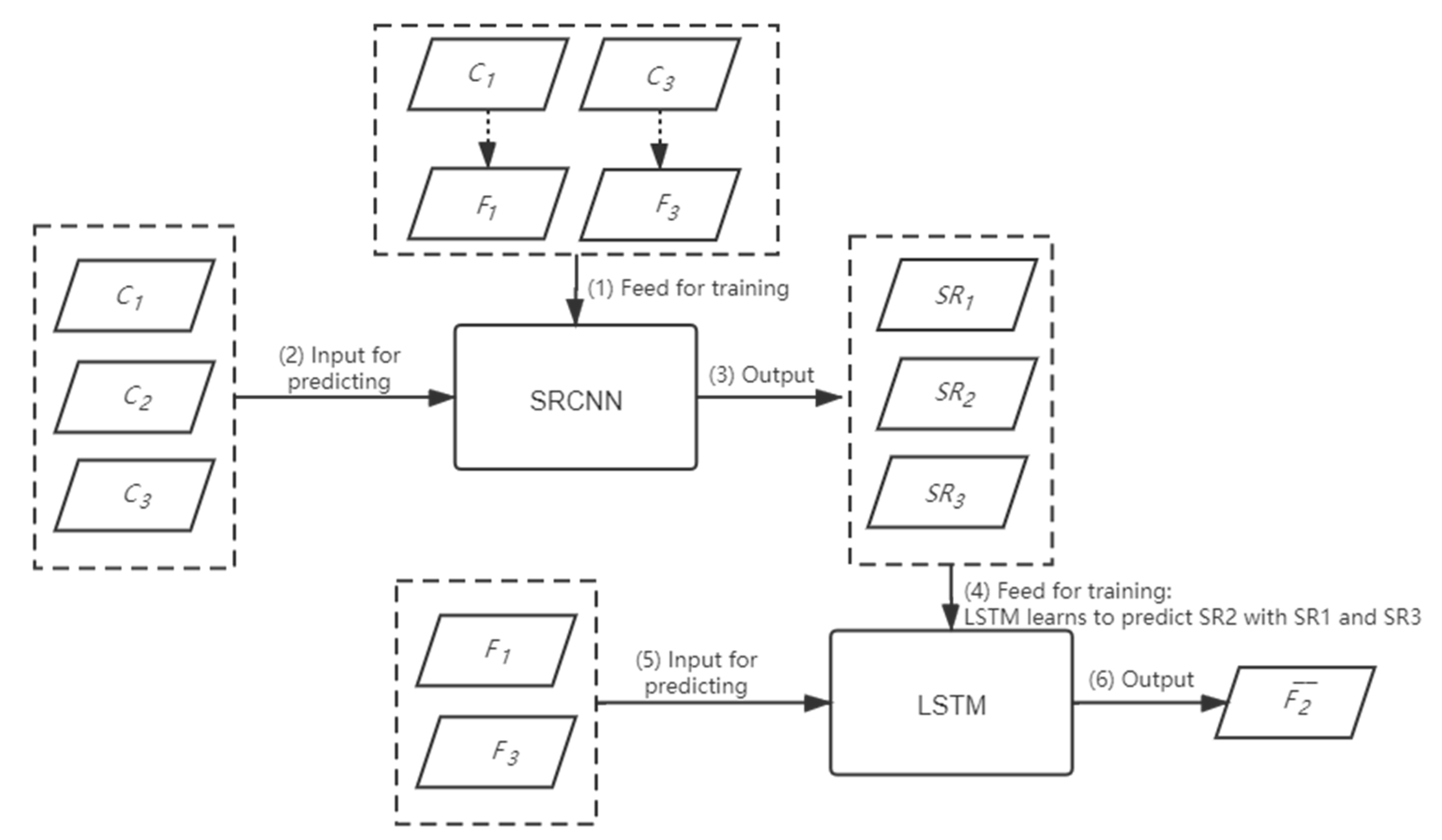
2.5. Hybrid Deep Learning Model

In this study, we develop a novel hybrid deep learning model for spatiotemporal fusion to better predict spatially detailed information and varying phenological changes in dynamic agricultural systems. Figure 2 shows the overall workflow of this study. The hybrid deep learning model integrates SRCNN and LSTM models: the SRCNN model is designed to enhance the spatial details using MODIS-Landsat image pairs, and the LSTM model will learn the phenological changing patterns in the enhanced images. We also design three scenarios representing different levels of temporal phenological changes among the fusion imagery. Those scenarios include rapid, moderate, and minimal phenological changes based on the transition dates in crop phenology. Then, the performance of the hybrid deep learning model is assessed under varying levels of phenological changes. Finally, three benchmark image fusion models, namely spatial and temporal adaptive reflectance fusion model (STARFM), flexible spatiotemporal data fusion (FSDAF), and STFDCNN, are selected to further evaluate the model performance.

The spatiotemporal image fusion involves the retrieval of two types of relationships: the spatial relationship between coarse MODIS and fine Landsat images, and the temporal relationship among the images acquired on different dates. Accurate retrievals of both spatial and temporal relationships are desired for favorable fusion modeling designs. In this study, we devise a hybrid deep learning modeling architecture that can accommodate both the relationships. Specifically, the hybrid deep learning model integrates the SRCNN and LSTM models. The SRCNN model is selected because of its ability to restore the degraded spatial information in the coarse images and to register the reflectance of the coarse and fine images using its convolution operations. The comparatively lightweight structure of SRCNN also makes the model suitable for mapping spatial features in satellite imagery while maintaining high computational efficiency [35]. With the registered reflectance and restored spatial information, the LSTM model is then designed to learn the temporal phenological changes among the SRCNN-derived imagery using its unique recurrent network structure.

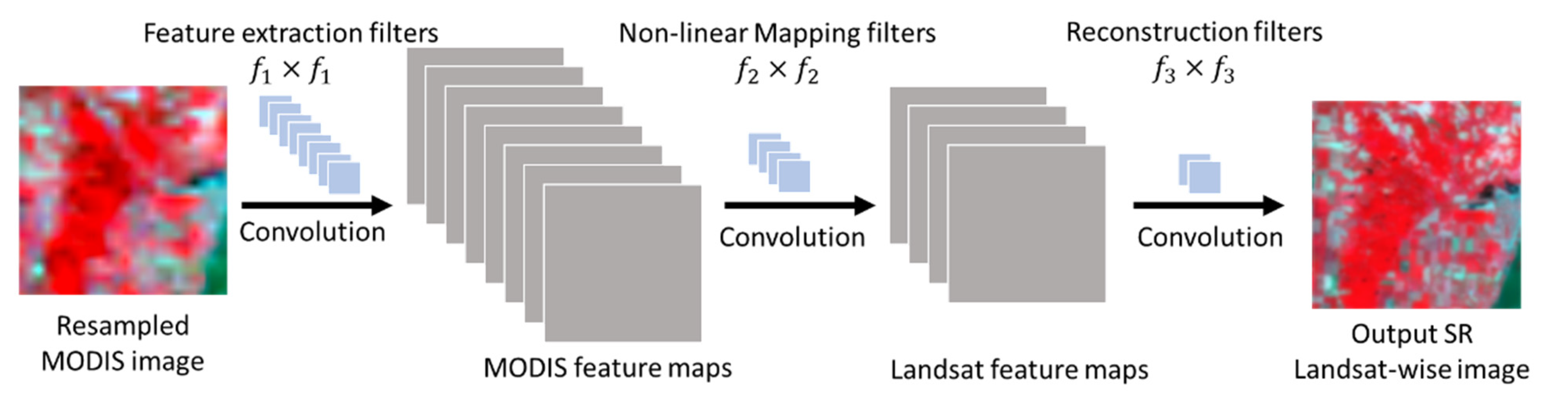
2.5.1. Hybrid Deep Learning Model: SRCNN

The SRCNN of the hybrid deep learning model is designed to learn the spatial relationship between coarse and fine images. SRCNN was initially proposed for image super- resolution [39]. It could extract image features from coarse images automatically and map those features non-linearly to reconstruct corresponding fine images. The SRCNN model contains three components: feature extraction, non-linear mapping, and reconstruction (Figure 3). The feature extraction component is to learn the critical spatial features from coarse MODIS images that have correspondence to fine Landsat images with convolution operations. The non-linear mapping component is to register the coarse MODIS and fine Landsat images, and to map the derived MODIS spatial features to corresponding features in fine Landsat images. The reconstruction component is to restore the degraded details in the coarse MODIS images, and to reconstruct super-resolution (SR) images of the coarse MODIS images at the Landsat scale. The SRCNN is trained with MODIS-Landsat image pairs on the image acquisition dates. Specifically, the coarse MODIS images are resampled to the dimensions of fine Landsat images using bilinear interpolation. Image pairs are then segmented into sub-image pairs to train the SRCNN model.

Through the feature extraction convolutional operation, the first hidden layer of SRCNN can be constructed with the rectified linear unit (ReLU) activation. ReLU is a computationally efficient activation function whose linear behavior will speed up the convergence of the network and alleviate the vanishing gradient problem. The results of the first hidden layer are the MODIS feature maps and are calculated according to the following equation:

$$U_1\left(C\right)=\max \left(0, W_1\ast C+B_1\right)$$

(1)

Here, C is the resampled coarse MODIS image segment. $W_1$ and $B_1$ are the weights and biases of the convolutional filters, respectively. The size of $W_1$ is $c\times f_1\times f_1\times n_1$, where C is the number of bands in the images (i.e., C = 6). The convolutional operation involves $n_1$ filters with the size of $f_1\times f_1$. The first hidden layer output $U_1\left(C\right)$ contains $n_1$ MODIS feature maps. Through optimizing $W_1$ and $B_1$, SRCNN can learn the most important spatial features of MODIS-Landsat relationships from the sub-image pairs.

The second hidden layer is constructed through the non-linear mapping convolutional operation, which maps the MODIS spatial features to the corresponding features in fine Landsat image segments. The sensor-induced reflectance differences can also be accommodated in this process. The results of the second hidden layer are the Landsat feature maps and are calculated according to the following equation:

$$U_2\left(C\right)=\max \left(0, W_2\ast U_1\left(C\right)+B_2\right)$$

(2)

Here, $W_2$ and $B_2$ are the weights and biases of the non-linear mapping convolutional filters, respectively. The size of $W_2$ is $n_1\times f_2\times f_2\times n_2$. This convolutional operation involves $n_2$ filters with the size of $f_2\times f_2$. The second hidden layer output $U_2\left(C\right)$ contains $n_2$ Landsat feature maps, which are generated from MODIS feature maps by optimizing $W_2$ and $B_2$.

The output layer is built through the reconstruction convolutional operation, which reconstructs the Landsat-wise SR image segment from the Landsat feature maps. The reconstruction operation can restore the deteriorated spatial patterns due to the coarsening of spatial resolutions. It recovers the spatial details of the input coarse MODIS image segment, and is calculated with the following equation:

$$U\left(C\right)=W_3\ast U_2\left(C\right)+B_3$$

(3)

Here, $W_3$ and $B_3$ are the weights and biases of the reconstruction convolutional filters, respectively. The size of is $n_2\times f_3\times f_3\times c$. There are $c$ filters with the size of $f_3\times f_3$ to reconstruct the image with c bands. The output $U\left(C\right)$ is the Landsat-wise SR image segment of the corresponding input MODIS image segment. In the training process, we attempt to minimize the difference between the estimated SR and reference fine Landsat image segments (F) using the loss function Loss. Loss is the average of mean square error (MSE) between those two image segments of all the training samples.

$$Loss(\Theta )=\frac{1}{n}{\displaystyle \sum }_{i=1}^n\left||U\left(C_i;\Theta \right)-F_i|\right|$$

(4)

where $n$ is the number of the training samples (segmented sub-images). $\Theta$ is the parameter set $\{W_1,W_2,W_3,B_1,B_2,B_3\}$ to be optimized. The size of a sub-image, the number of filters, and the corresponding size in each convolution layer are set through balancing the network performance and computational cost. With a multitude of parameter tuning in reference to previous studies, the sub-image dimension is set to be 33 × 33, with the hyperparameters $\{f_1,f_2,f_3,n_1,n_2,c\}$ set to be $f_1=9, f_2=5, f_3=5, n_1=64, n_2=32, c=6$ [22]. With the trained SRCNN model, the Landsat-wise SR images on both image acquisition and prediction dates can be reconstructed from the corresponding MODIS images.

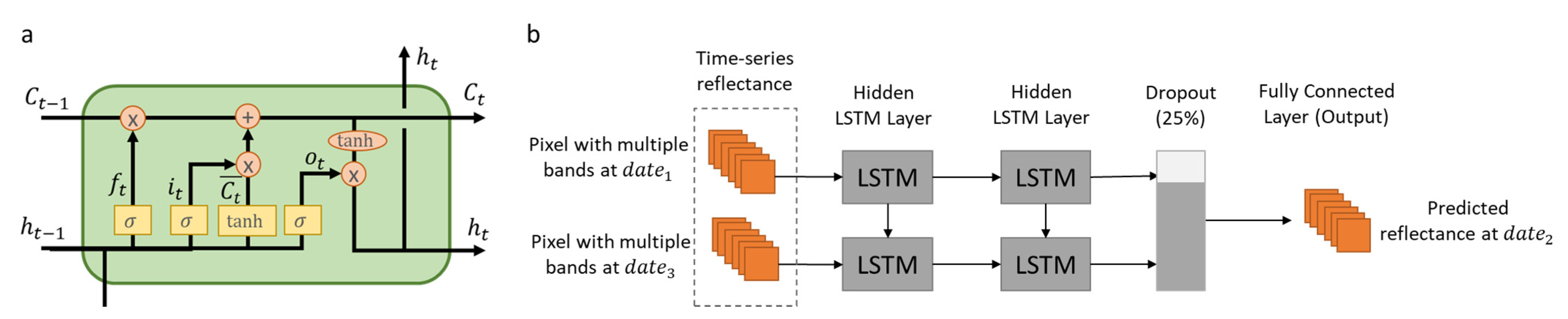
2.5.2. Hybrid Deep Learning Model: LSTM

The LSTM of the hybrid deep learning model is designed to learn the temporal phenological patterns from a sequence of images. LSTM handles the vanishing gradient problem encountered in RNN, and improves the network cell structure with the gating mechanism that enables the information to be stored in memory for longer periods. It regulates the flow of temporally evolving information by selectively preserving the memory and adding new information to model the temporal changing patterns underlying the sequential data. Through the combined use of various gates and memory cells, LSTM can learn the temporal evolving features from a sequence of images for time series prediction. The unique structure of LSTM thus shows great potential to characterize complex temporal phenological changes among the satellite imagery for spatiotemporal image fusion. A typical LSTM cell unit consists of cell state, input gate, forget gate, and output gate to control the propagation of information (Figure 4a). With the regulation of those gates, the memory stored in the cell state will be selectively updated or removed over time [32].

At time step t, the LSTM unit updates the cell state ($C_t$) and hidden state ($h_t$), according to the previous cell state ($C_{t-1}$); the previous hidden state ($h_{t-1}$); the current input ($S{R}_t$); and a combination of forget (f_t), input (i_t), and output ($o_t$) gates. Specifically, the forget gate ($f_t$) controls the amount of the information in the previous cell state to be discarded (Equation (5)), and the input gate (i_t) regulates the level of new information to be added into the memory cell (Equation (6)).

$$f_t=\sigma (W_{fSR}S{R}_t+W_{fh}{h}_{t-1}+b_f)$$

(5)

$$i_t=\sigma (W_{iSR}S{R}_t+W_{ih}{h}_{t-1}+b_i)$$

(6)

Here, $f_t$ is the forget gate with values ranging from 0 to 1. Larger values of the forget gate indicate larger amount of information in the previous memory cell to be retained. $S{R}_t$ is the new pixel-based six-band spectral input from the Landsat-wise SR images at time step t, and $h_{t-1}$ is the previous hidden state. $W_{f\ast }$ and $b_f$ denote the weights and the bias of the forget gate, respectively. Comparably, is the input gate that has values between 0 and 1, with larger values indicating a higher level of new information to flow into the memory cell. $W_{i\ast }$ and $b_i$ are the weights and the bias of the input gate, respectively. $\sigma$ is the sigmoid activation function to scale the gate values between 0 and 1, with 0 representing no flow and 1 being complete flow of information throughout the gates.

With the forget gate ($f_t)$ and the input gate ($i_t$), the cell state ($C_t$) will be updated through weighting the memory of the previous cell state and newly added information (Equation (7)).

$$C_t=f_t·C_{t-1}+i_t·\overline{C_t}$$

(7)

$$\overline{C_t}=tanh\left(W_{cSR}S{R}_t+W_{ch}{h}_{t-1}+b_c\right)$$

(8)

Here, $C_t$ is the updated cell state at time step t, which is the summation of the previous cell state ($C_{t-1}$) pointwise multiplied by the forget gate ($f_t$), and the candidate cell state ($\overline{C_t}$) pointwise multiplied by the input gate ($i_t$). The candidate cell state ($\overline{C_t}$) contains the new information that is considered to be added into the cell memory. The hyperbolic tangent activation function ($tanh$) is employed to scale the values of $\overline{C_t}$ to the range from −1 to 1 for regulating the network. $W_{c\ast }$ and $b_c$ are the weights and the bias of the candidate cell state, respectively. With the regulation of forget and input gates, the updated cell state will forget part of existing memory while adding a new memory.

The output gate ($o_t$) regulates the amount of the updated cell state ($C_t$) in computing the updated hidden state ($h_t)$ at time step t (Equations (9) and (10)).

$$o_t=\sigma (W_{oSR}S{R}_t+W_{oh}{h}_{t-1}+b_o)$$

(9)

$$h_t=o_t·tanh\left(C_t\right)$$

(10)

Here, $o_t$ is the output gate that has values ranging from 0 to 1, with higher values indicating larger amount of the cell state memory ($C_t$) in updating the hidden state (h_t). $W_{o\ast }$ and $b_o$ denote the weights and the bias of the output gate, respectively. The updated cell state ($C_t$) and updated hidden state ($h_t$) will be carried over to the next time step t + 1.

With the cell state and gates design, the LSTM model can regulate the propagation of information over time and retrieve the temporal evolving features characteristic of temporal phenological changes from the multi-date satellite images. Constructed on a per-pixel basis, the model can selectively preserve and discard the spectral reflectance information to learn its changing patterns among the imagery through a combination of forget, input, and output gates. Activation functions (e.g., sigmoid function and hyperbolic tangent function) further enhance the model’s capability to capture complex and non-linear temporal dependencies among the multi-date imagery. In this study, the LSTM model is trained using the SRCNN-derived multi-date Landsat-wise SR images to characterize the temporal dependencies between the spectral reflectance on the prediction date and that on the image pair acquisition dates. The learned knowledge from the multi-date SR images will be applied to the corresponding Landsat images to generate final fusion predictions. Figure 4b shows the structure of the LSTM model in this study. The LSTM model comprises two LSTM layers, each with 100 LSTM cell units to retrieve the temporal features characteristic of spectral reflectance changes. A dropout layer is designed after the two LSTM layers with a dropping rate of 25% to overcome the potential overfitting, and then a fully connected layer is constructed for generating the fused Landsat-wise image on the prediction date. The model parameters (e.g., weights and biases) are optimized using Adam through balancing between the model accuracy and computational cost.

The hybrid deep learning model is tested with both simulation dataset and real MODIS-Landsat image pairs. To make the results comparable with the benchmark models, only two image pairs and one coarse image acquired on the prediction date are employed in this study to construct the hybrid deep learning model. However, more image pairs can be accommodated in the proposed model. Figure 5 shows the workflow of the proposed hybrid deep learning model. Suppose there are coarse images $C_1,C_2, \mathrm{and} C_3$ at dates 1, 2, and 3, respectively. There are also fine images $F_1$ and $F_3$ acquired at date 1 and date 3, respectively. The fusion model will predict the fine image $\overline{F_2}$ at date 2, given the image pairs $C_1~F_1$ and $C_3~F_3$, and the coarse image $C_2$ on the prediction date. First, the SRCNN model is constructed according to the image pairs $C_1~F_1$ and $C_3~F_3$. With the trained SRCNN model, three SR images, $S{R}_1,S{R}_2$, and $S{R}_3$, can be estimated from coarse images $C_1,C_2, \mathrm{and} C_3$, respectively. Then, the LSTM model will be constructed to learn the temporal change information from the sequence of images $S{R}_1$ and $S{R}_3$ to predict $S{R}_2$. The learned LSTM model can then be employed to predict the fine image $\overline{F_2}$ with the sequence of fine images $F_1$ and $F_3$.

2.5.3. Implementation of the Hybrid Deep Learning Model

The hybrid deep learning model is implemented using the Keras library with a Tensorflow backend. The training and testing processes are run on an NVIDIA GK110 “Kepler” K20X GPU accelerator. The optimizer used in the hybrid model is Adam with adaptive learning rates. The initial learning rate is set empirically as 0.001. For SRCNN, sub-images are regularly clipped from the original images; 10,000 sub-images are randomly used for training and 2500 sub-images are reserved for testing. For LSTM, 150,000 pixels are randomly selected from the image for training, while 30,000 random pixels are used for testing. The mini-batch size is set to be 128 to fit in the GPU memory. Other hyperparameters regarding the model structures are described in Section 3.2.1 and Section 3.2.2. The SRCNN and LSTM models are trained for 50 and 150 epochs to converge in the main study site, respectively. In terms of running time, each epoch for the SRCNN and LSTM model costs about 3 and 25 s, respectively (around 60 min for each three-date image combination). Most model parameters could be applied to the different test sites, while the number of training epochs may need to be adjusted to ensure the convergence of models.

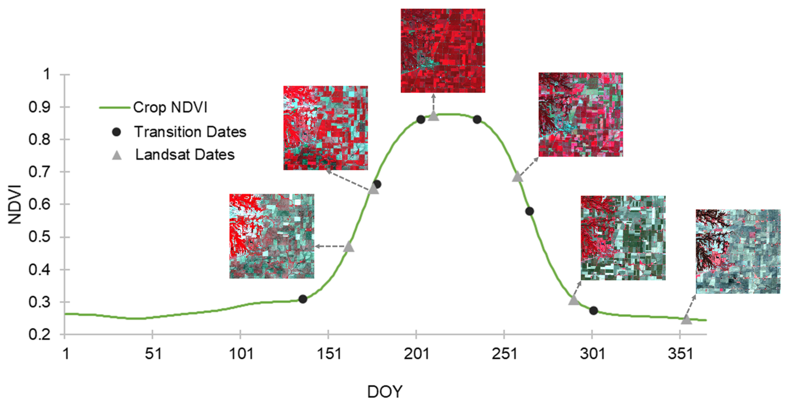
2.6. Design of Phenological Change Scenarios

To evaluate varying levels of phenological changes’ impacts on fusion models, we design the scenarios of rapid/moderate/minimal phenological changes based on the phenology information in the images. As corn and soybeans take up more than 70% of our main study site (Table S1), we use averaged phenology information of all crop (corn and soybeans) pixels throughout the main study site to identify critical phenological transition dates, and then the three scenarios are determined based on the relationships between image acquisition dates and the phenological transition dates. Averaged phenology information is adopted here as we assume that the average phenology of the main land cover types could represent the general temporal phenological trends of the site. Specifically, the critical phenological transition dates are identified by the remote sensing phenological monitoring framework proposed by Diao [7]. The double logistic model is applied on the smoothed daily mean normalized difference vegetation index (NDVI) of the crop pixels derived from MODIS images [40]. The phenological transition dates are the timings corresponding to the local minima or maxima of the first derivative of the NDVI time series, or the extremes of the change rates in the NDVI time series’ curvature [7]. Those transition dates mark the average timings of crops transitioning from one phenological stage to another, and they are utilized to divide the satellite imagery into different phenological stages. With those identified transition dates, we design three phenological change scenarios. Suppose we have two image pairs on dates $t_1$ and $t_3$, respectively, and the coarse image on $t_2$. The three scenarios are (1) rapid phenological changes (i.e., rapid), where the three dates $t_1$, $t_2$, and $t_3$ are at three different phenological stages; (2) moderate phenological changes (i.e., moderate), where $t_1$ and $t_3$ are at two different stages, and $t_2$ shares the same stage with either $t_1$ or $t_3$; and (3) minimal phenological changes (i.e., minimal), where all the three dates $t_1$, $t_2$, and $t_3$ are at the same phenological stage.

By designing the three scenarios, we attempt to examine how the fusion models respond to different levels of phenological changes. As we use two image pairs acquired before and after the prediction dates, we refer two image pairs as “bracketing images”. The “minimal” scenario is to mimic the situation when there is minimal phenological change between the bracketing images. The “moderate” scenario represents the situation when phenological changes are present, yet one bracketing image records these changes to some extents. The “rapid” scenario stands for the situation when the changes are so fast and/or transient and no bracketing images can capture such changes. For both real satellite and simulation data, the results will be presented and discussed by different scenarios to help better understand how the fusion models perform under different circumstances of phenological changes.

2.7. Benchmark Fusion Models

In this study, our proposed hybrid model is compared with three benchmark models: STARFM, FSDAF, and STFDCNN. To ensure the results from different fusion models are comparable, all the models utilize two image pairs and the coarse image on the prediction date to estimate the corresponding fine image on that date.

STARFM is a classic weight function-based spatiotemporal image fusion model [12]. It assumes that the change in surface reflectance between the coarse and fine images is equivalent and that the sensor difference is consistent among the imagery. For each to-be-predicted fine pixel, STARFM searches for spectrally similar pixels within a moving window in the fine images as candidate pixels. Weights are given to candidate pixels based on spectral difference between the coarse and fine images, temporal difference between image acquisition dates, and spatial distance between the predicted pixel and candidate pixels. The prediction is the weighted average of those similar pixels.

FSDAF integrates the weight function-based and unmixing-based approaches to provide more flexible predictions of both gradual and abrupt changes in heterogeneous landscapes [23]. An unmixing approach is first adopted to predict temporal changes in the fine images. Residuals of the temporal prediction are subsequently distributed to the fine pixels using a thin plate spline interpolator. A weight function is then applied to the distributed residuals and temporal changes, based on spectral difference and spatial distance, to obtain the final predictions. The two predicted fine images from the two image pairs are synthesized as suggested in Zhu, Helmer, Gao, Liu, Chen, and Lefsky [23].

STFDCNN utilizes deep CNN models to fuse coarse and fine images [22]. The CNN models restore the spatial details in the coarse images, and the outputs of CNNs are transitional images. A high-pass modulation is adopted to derive the spatiotemporal relationship among the imagery with the integrated use of the original fine images and transitional images, and to predict the fine image of the target date.

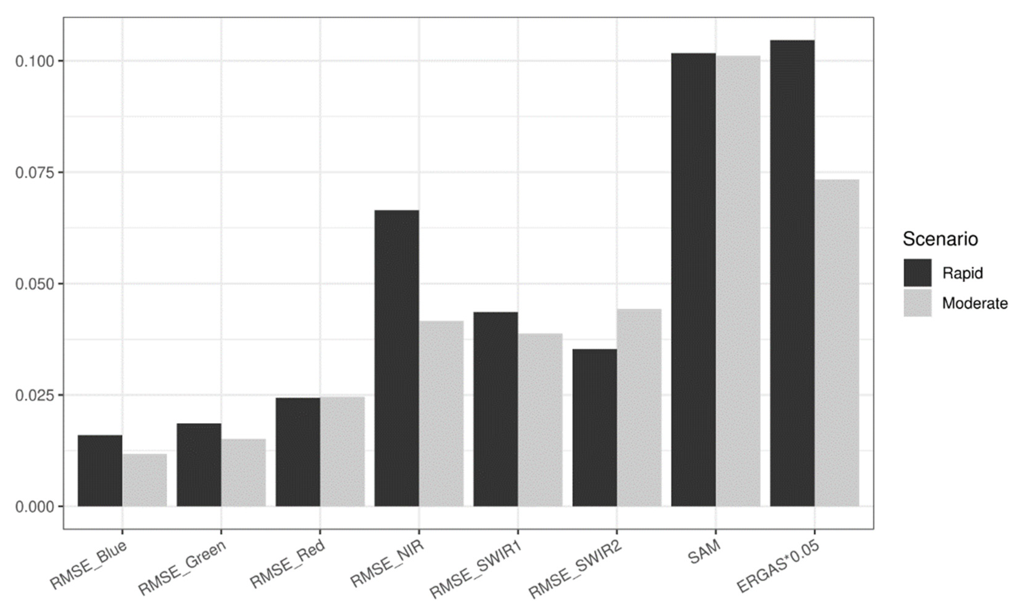
2.8. Accuracy Assessment

To evaluate the fusion results, three quantitative indices are used in this study. The first index is root mean square error (RMSE), which calculates the average reflectance difference between the predicted image and the reference image. RMSE is calculated for every single band with the following equation:

$$\mathrm{RMSE}=\sqrt{\frac{{{\displaystyle \sum }}_{i=1}^R{{\displaystyle \sum }}_{j=1}^C{\left({\widehat{L}}_{ij}-L_{ij}\right)}^2}{R\times C}}$$

(11)

Here R and C denote the numbers of rows and columns of the image. $\widehat{L}$ and $L$ represent the reflectance of a certain band of the predicted image and the reference image, respectively.

The other two indices are spectral angle mapper (SAM) and erreur relative global adimensionnelle de synthese (ERGAS) [41]. Complementary to RMSE, those two indices are cross-band measures and can evaluate the fusion results on a multiple band basis. ERGAS assesses the spectral difference between the predicted and the reference images in terms of normalized RMSE across bands. It can accommodate the inherent differences in the reflectance values among different bands, as well as the magnitude of the resolution difference between the fine and coarse images. The definition is as follows:

$$\mathrm{ERGAS}=100\frac{h}{l}\sqrt{\frac{1}{M}{{\displaystyle \sum }}_{b=1}^M[\mathrm{RMSE}{\left({\widehat{L}}_b\right)}^2/{\mu }_b{}^2]}$$

(12)

Here h and l are the spatial resolutions of fine and coarse images, respectively; $M$ denotes the number of bands. ${\widehat{L}}_b$ stands for the predicted reflectance values for band $b$, and ${\mu }_b$ is the mean value of band $b$ of the image.

SAM is used to measure the spectral distortion of the predicted image upon comparison to the reference image on a multi-band basis. The spectral information of each pixel can be viewed as an N-dimensional spectrum vector. The spectral distortion is measured as the N-dimensional vector angle between the predicted and the reference spectra of the pixel. SAM is the mean of all pixels’ N-dimensional vector angles, with smaller values indicating that the spectral information of the predicted image is closer to that of the reference image. It is defined as:

$$\mathrm{SAM}=\frac{1}{N}{\displaystyle \sum }_{n=1}^{N}arccos\frac{{{\displaystyle \sum }}_{b=1}^M\left({\widehat{L}}_n^b{L}_n^b\right)}{\sqrt{{{\displaystyle \sum }}_{b=1}^M{\left({\widehat{L}}_n^b\right)}^2{{\displaystyle \sum }}_{b=1}^M{\left(L_n^b\right)}^2}}$$

(13)

Here $N$ is the total number of the pixels in the image. ${\widehat{L}}_n^b$ and $L_n^b$ stand for the reflectance for pixel n in band b of the predicted image and the reference image, respectively.

3. Results

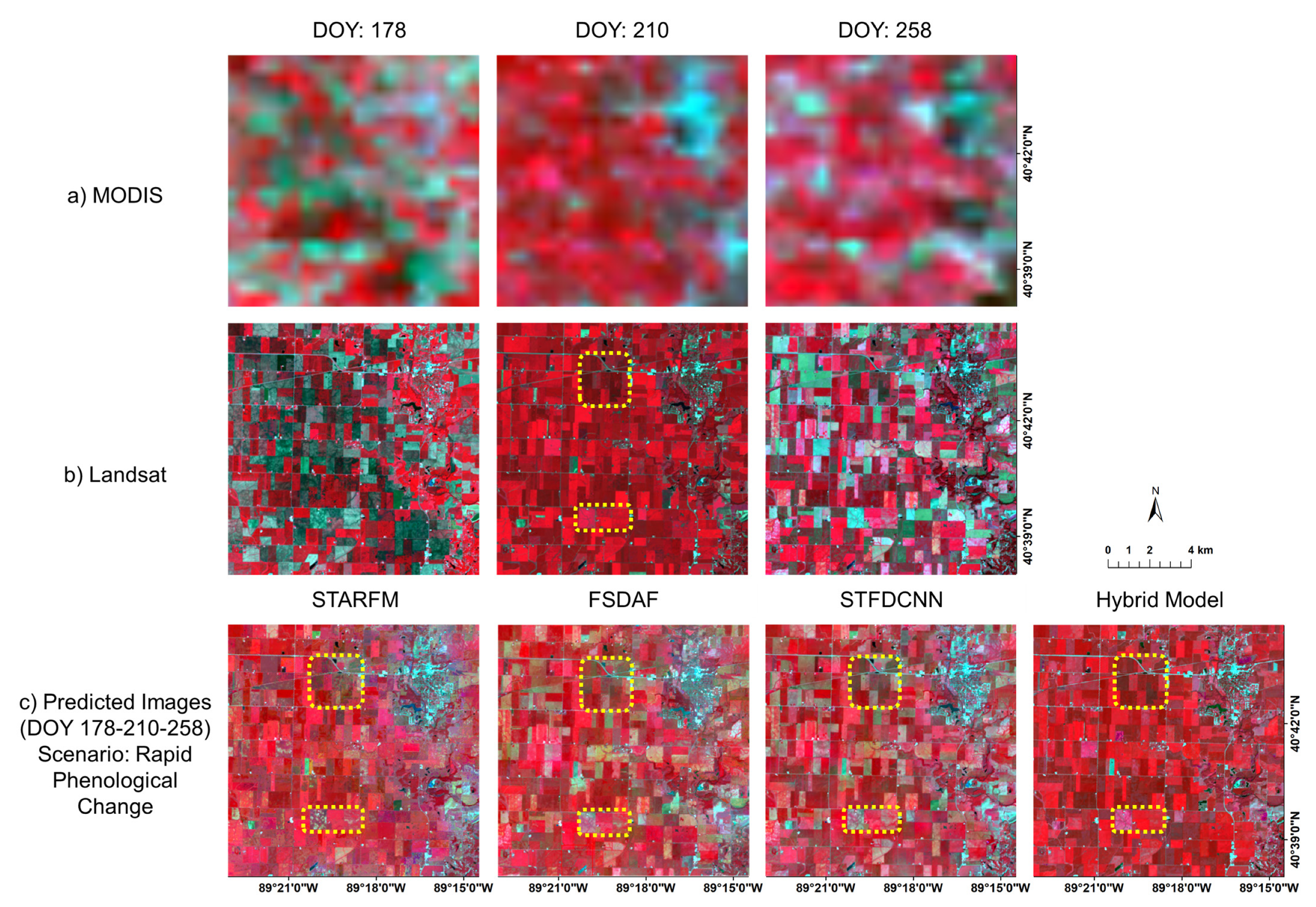
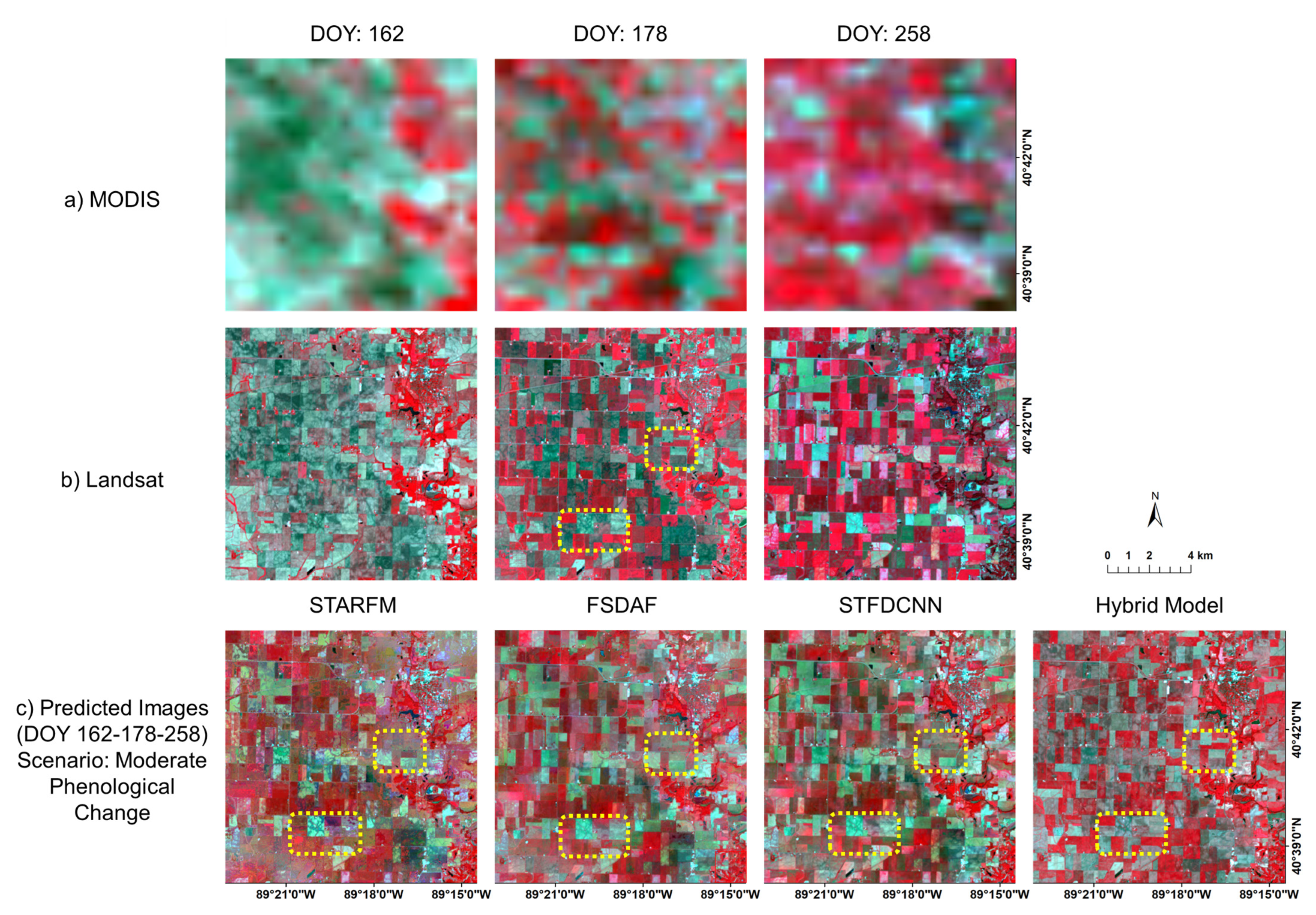
3.1. Scenarios of Phenological Changes

Six phenological transition dates are identified by the phenological monitoring framework [7] based on the average NDVI curve of all the crop pixels generated from MODIS in the main study site. The transition dates are: DOY 136, 179, 203, 235, 265, and 301. Figure 6 shows the transition dates along with the average crop NDVI curve. These six transition dates divide the year into seven stages. Note that the six Landsat images in this study are mostly at different stages, except the first two dates, DOY 162 and 178, falling in the same stage (Figure 6 and Figure S4). This indicates that, in real-world situations, the rapid phenological change scenario is common, especially during the growing season.

A total of 20 three-date image combinations are made from the six Landsat images. The four combinations containing DOY 162 and 178 are considered as the combinations of “moderate phenological changes”. The other 16 combinations are categorized as “rapid phenological changes”. We do not have “minimal phenological changes” combinations for satellite images, as there are no three satellite images at the same phenological stage. For simulation data, we make eight “rapid phenological changes” combinations, five “moderate phenological changes” combinations, and four “minimal phenological changes” combinations. Considering that Landsat has a 16-day revisit cycle, we attempt to avoid picking two dates that are too close to each other when testing with simulation data, as an effort to imitate the real-world situations. The fact that some intervals between the transition dates are quite narrow limits our ability to choose images for the “minimal” scenario. Thus, the numbers of cases for simulation data in different scenarios are not the same.

3.2. Fusion Results of Hybrid Deep Learning Model

3.2.1. Simulation Data

We test the hybrid model on simulation data to evaluate whether it can accurately predict spatiotemporal features and whether it is robust faced with various levels of phenological changes. The hybrid deep learning model demonstrates its robustness by generating satisfactory results in all three phenological change scenarios (Figure S5a–c). The predicted images by the hybrid deep learning model resemble the reference images in terms of both spectral information and spatial details. Figure 7 provides the summarized quantitative measures for the 17 simulated image combinations of the three scenarios. The mean RMSE values for all the scenarios are lower than 0.005 for visible bands and lower than 0.01 for infrared (IR) bands. The mean SAM and ERGAS values for all the scenarios also suggest low errors. To test if the model is robust to various levels of changes, one-way ANOVA tests are conducted on RMSE by band, SAM, and ERGAS. The test results reveal that all the metrics show no significant differences with regard to different levels of phenological changes. Both the visual examples and quantitative measures indicate that the hybrid deep learning model can provide accurate predictions of spatial and temporal features and retain its excellent performance under various levels of temporal phenological changes.

3.2.2. Satellite Data

We also test how the model performs with real satellite images and whether the real satellite results concur with the simulation results. Compared to the simulated data, the real satellite images are much more spatially heterogeneous and embody more complex temporal changes. The hybrid deep learning model again demonstrates its ability to robustly predict the spatial and temporal features in both “rapid” and “moderate” scenarios (Figure S6). Figure 8 shows the summarized quantitative results of the 20 real satellite image combinations of those two scenarios using RMSE, SAM, and ERGAS. Errors are generally low (mean RMSE < 0.025 for visible bands and < 0.07 for IR bands), though they are higher than the simulation results. One-way ANOVA tests suggest that the RMSE values exhibit no significant difference regarding different levels of phenological changes in green (p = 0.076), red (p = 0.077), and SWIR1 (p = 0.343) bands, whereas the RMSE values in blue (p = 0.001), NIR (p = 0.004), and SWIR2 (p = 0.006) bands show significant differences for different scenarios. The ERGAS measures also show significant difference (p = 0.003). The SAM values, on the other hand, present no significant difference (p = 0.948). Admittedly, significant differences are observed in some metrics due to the increased complexity of the real satellite images, yet the hybrid deep learning model still holds its robustness in certain aspects. For instance, the insignificant difference of SAM indicates that the hybrid deep learning model is especially robust in predicting the spectral information and controlling spectral distortion.

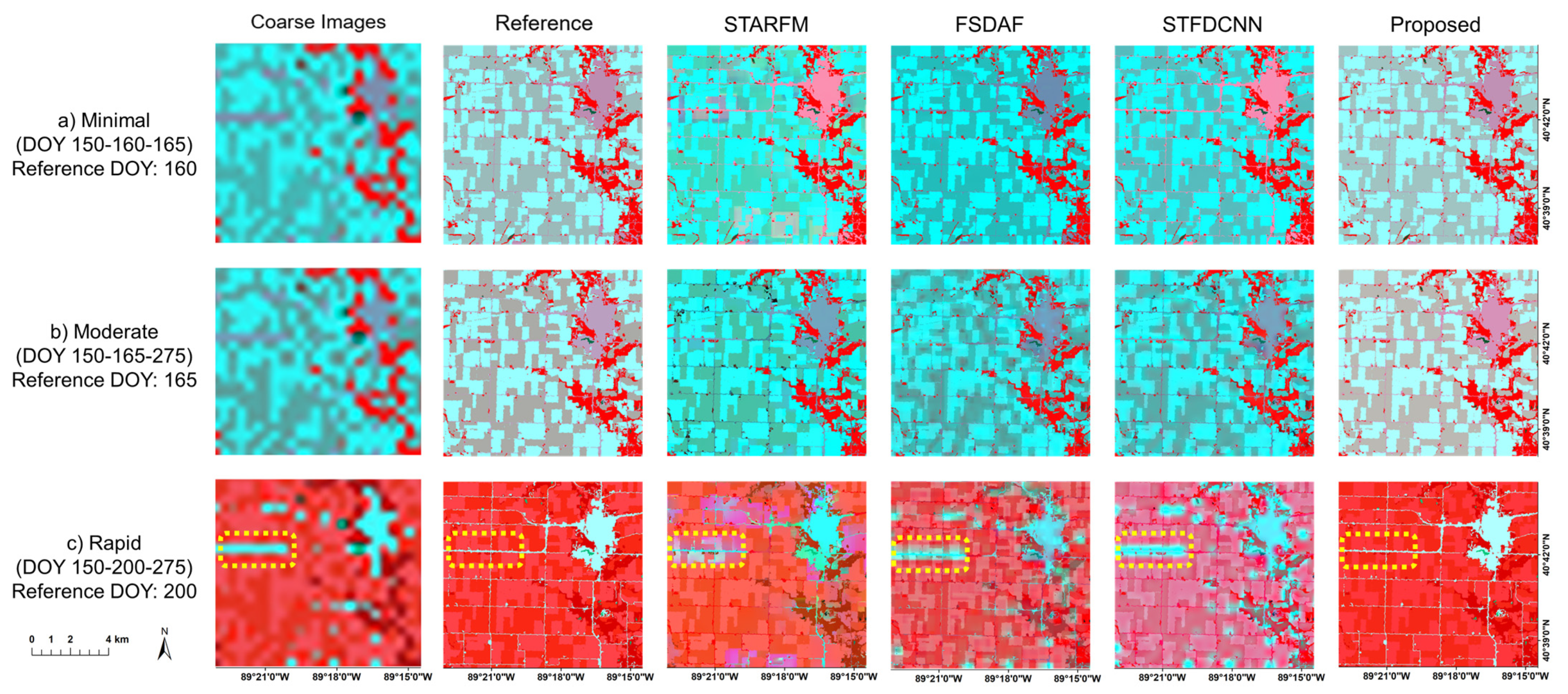
3.3. Comparison with Benchmark Models

To comprehensively assess the fusion models and provide instructional insights for model selection and improvement, we carry out a comparison among our hybrid deep learning model and three benchmark models (STARFM, FSDAF, and STFDCNN), using both simulation and satellite data.

3.3.1. Comparison Results of Simulation Data

Figure 9a–c show visual segment examples of the “minimal”, “moderate”, and “rapid” scenarios using simulation data, respectively. In the “minimal” scenario, spatial details and spectral information are well preserved by all the methods. In the “moderate” scenario, we start to observe blurring effects especially for crop fields in FSDAF and STFDCNN. Model performances are further degraded in the “rapid” scenario—the three benchmarks exhibit distortions in both spatial details and spectral information, while the hybrid deep learning model remains robust. In general, the images fused by our hybrid model are more consistent with the reference images compared to those generated by the benchmark models. It is also noted that the hybrid deep learning model can better handle the large spatial resolution discrepancy between MODIS and Landsat, as the yellow dashed rectangles in Figure 9c illustrate.

As for the quantitative measures of the 17 simulated image combinations, Figure 10a–f show the average RMSE for each band. Figure 10g,h show the average SAM and ERGAS values, respectively, which are also presented in

Table 1. Cross-band accuracy metrics (SAM and ERGAS) for experiments using simulation data. Bold fonts represent more favorable results.

SAM				Simulation Data	ERGAS
STARFM	FSDAF	STFDCNN	Proposed	Scenario	STARFM	FSDAF	STFDCNN	Proposed
0.0446	0.0584	0.0591	0.0243	Rapid	0.9518	0.9273	1.6172	0.3027
0.0302	0.0256	0.0216	0.0221	Moderate	0.4623	0.2940	0.3494	0.2721
0.0105	0.0114	0.0203	0.0230	Minimal	0.1404	0.1405	0.1200	0.2694
0.0323	0.0380	0.0389	0.0234	Overall	0.6169	0.5559	0.8920	0.2859

. The error bars represent the standard errors. All the accuracy metrics are presented by the three phenological change scenarios, and the “overall” accuracy is the average of all the 17 experiments regardless of the scenarios. A general trend that we observe is that the “rapid” scenario gives rise to the highest errors, and the “minimal” scenario has lowest errors, with the “moderate” scenario falling between. For the overall accuracy, the hybrid deep learning model achieves the lowest errors (SAM: 0.0234 and ERGAS: 0.2859), while other three models produce generally larger errors. The error bars indicate that the hybrid model generates the least overall variability. The hybrid model demonstrates a better overall performance of the 17 simulation experiments.

In the “rapid” scenario, the hybrid model yields the lowest errors (ERGAS = 0.3027, SAM = 0.0243) in all metrics. FSDAF (ERGAS = 0.9273, SAM = 0.0584) is the second-best model among the four in terms of ERGAS, while STARFM (ERGAS = 0.9518, SAM = 0.0446) achieves lower SAM compared to FSDAF. Since STFDCNN emphasizes more on the spatial domain, this model design may be less ideal for handling rapid phenological changes (ERGAS = 1.6172, SAM = 0.0591). In the “moderate” scenario, the hybrid deep learning model exhibits the lowest RMSE in green, NIR, and SWIR1 bands and the lowest ERGAS. FSDAF generates the lowest RMSE in the other three bands and the second-lowest ERGAS. As the desired fusion models ranked by different metrics may vary, it may be difficult to pinpoint the unanimously best model in the “moderate” scenario. Yet the hybrid deep learning model and FSDAF (ERGAS: 0.2721 and 0.2940, respectively) should be among the best overall. As the level of phenological changes decreases, we find that STFDCNN performs remarkably better than that in the “rapid” scenario. In the “minimal” scenario, all the four methods achieve low errors. The hybrid deep learning model yields the highest error in the “minimal” scenario. The higher errors are mostly due to deep learning models’ sensitivity to the signal to noise ratio (SNR); when there is minimal phenological change, SNR gets lower. The lower SNR will degrade the deep learning model’s performance [42].

In summary, the hybrid deep learning model yields more favorable results compared to other models in the “rapid” and “moderate” scenarios, while yielding higher errors than other models in the “minimal” scenario. The hybrid model also exhibits the most robust performances when levels of phenological changes vary.

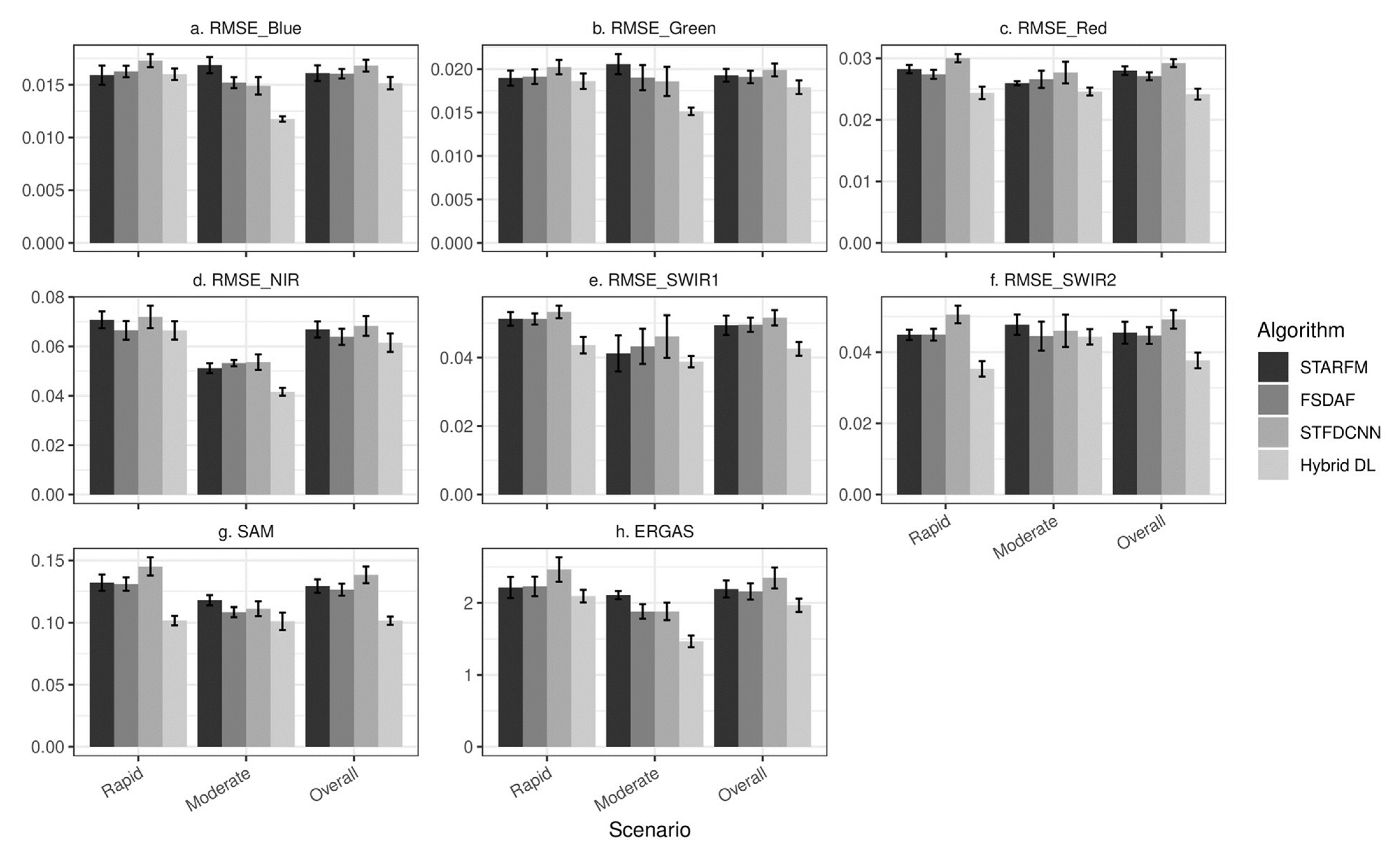
3.3.2. Comparison Results of Satellite Data

Figure 11 and Figure 12 show segment examples of satellite image results. Figure 11 shows the results for the combination of DOY 178-210-258 in false color composite, categorized as “rapid”. Specifically, Figure 11c shows the fusion results of the four models. Note that the reference image is the Landsat image on DOY 210. We find that the hybrid deep learning model successfully captures the temporal phenological changes of the crop fields while retaining spatial details, such as boundaries and roads. STARFM exhibits blurring effects, whereas FSDAF and STFDCNN show biases in spectral information (see yellow rectangular areas in Figure 11c). Figure 12 shows the results for the combination of DOY162-178-258 in the false color composite, which belongs to the “moderate” scenario. The reference image is the Landsat image on DOY 178. The predicted image by the hybrid deep learning model best resembles the reference image. STARFM, similar to the example in “rapid” scenario, suffers from the blurring effects. FSDAF and STFDCNN preserve spatial details well, but are relatively flawed in predicting temporal phenological changes (see yellow rectangular areas in Figure 12c).

With regards to the quantitative measures of the 20 satellite image combinations, Figure 13a–f show the average RMSE for each band. Figure 13g,h show the average SAM and ERGAS, respectively, which are also presented in

Table 2. Cross-band accuracy metrics (SAM and ERGAS) for experiments using satellite data. Bold fonts represent more favorable results.

SAM				Real Data	ERGAS
STARFM	FSDAF	STFDCNN	Proposed	Scenario	STARFM	FSDAF	STFDCNN	Proposed
0.1321	0.1309	0.1451	0.1044	Rapid	2.2124	2.2268	2.4626	2.1306
0.1179	0.1084	0.1111	0.1043	Moderate	2.1063	1.8819	1.8824	1.4834
0.1292	0.1264	0.1383	0.1044	Overall	2.1912	2.1578	2.3466	2.0012

. The error bars stand for standard errors. Similar to the simulation results, the errors are generally higher in the “rapid” scenario than those in the “moderate” scenario. Yet the contrast between these two scenarios is not as drastic as that in the simulation results. The reason could be that the satellite data are more complicated than the simulation data, and the errors could come from the sources other than inaccurate prediction of phenological changes. For example, the more heterogeneous spatial landscape and more complex temporal phenological change patterns will pose greater challenges to the fusion models. Thus, controlling the levels of phenological changes may not have the same magnitude of effects on prediction accuracy in satellite image results as that in simulation results. For the overall accuracy, the hybrid deep learning model achieves the lowest errors (SAM: 0.1044 and ERGAS: 2.0012), followed by FSDAF (SAM: 0.1264 and ERGAS: 2.1578). The hybrid deep learning model remains the overall best-performing model and achieves the lowest standard errors for both the cross-band metrics (SAM and ERGAS) in the 20 combination experiments using satellite images.

In the “rapid” scenario, the hybrid deep learning model achieves the lowest SAM (0.1044), ERGAS (2.1306), and RMSE for almost all the bands except the blue band (STARFM: 0.159 vs. hybrid deep learning: 0.160) (Table 2 and Figure 13). Among the benchmark models, STARFM (SAM = 0.1321, ERGAS = 2.2124) and FSDAF (SAM = 0.1309, ERGAS = 2.2268) are more accurate than STFDCNN in capturing rapid phenological changes, similar to simulation results. In the “moderate” scenario, the hybrid deep learning model maintains its leading position, and presents the lowest errors for all the metrics (SAM = 0.1043, ERGAS = 1.4834). STARFM in the “moderate” scenario generates less favorable results compared to FSDAF and STFDCNN. In general, the accuracy results of real satellite images match the patterns shown in simulation results. As the real satellite images are more complicated than simulation data, this comparative analysis demonstrates the improved capability of the hybrid deep learning model in learning complex spatiotemporal features and predicting complicated temporal phenological changes.

To further compare the overall performance of those four models, pairwise t-tests with Bonferroni-adjusted p-values are conducted (

Table 3. Results of pairwise comparisons using paired t-tests with Bonferroni-adjusted p-values. Comparisons include the proposed model vs. STARFM, FSDAF, and STFDCNN.

Hybrid Model vs.	STARFM	FSDAF	STFDCNN
SAM	p < 0.001	p < 0.001	p < 0.001
ERGAS	p = 0.022	p = 0.011	p < 0.001

). The results indicate that the hybrid model generates significant better fusion results than the three benchmark models, using SAM and ERGAS as assessing metrics.

3.4. Fusion Results in Additional Test Sites

In addition to the main study site, we select three additional study sites (the Oklahoma site, the Chicago site, and the Harvard Forest site) to assess the generalization ability of the hybrid deep learning model.

Table 4. Cross-band accuracy metrics (SAM and ERGAS) for experiments in additional test sites. Bold fonts represent more favorable results.

SAM					ERGAS
STARFM	FSDAF	STFDCNN	Proposed	Site: Oklahoma	STARFM	FSDAF	STFDCNN	Proposed
0.1256	0.1123	0.1143	0.0990	Rapid	1.9885	1.8825	1.9133	1.8506
0.0956	0.0786	0.0784	0.0693	Moderate	1.4872	1.3209	1.3065	1.2558
0.1136	0.0988	0.0999	0.0871	Overall	1.7880	1.6578	1.6706	1.6127
STARFM	FSDAF	STFDCNN	Proposed	Site: Chicago	STARFM	FSDAF	STFDCNN	Proposed
0.1400	0.1276	0.1360	0.1281	Rapid	2.8813	2.8281	2.8452	2.7232
0.1077	0.1140	0.1131	0.1109	Moderate	2.3977	2.3196	3.1150	2.2776
0.1206	0.1194	0.1222	0.1178	Overall	2.5911	2.5230	3.0071	2.4559
STARFM	FSDAF	STFDCNN	Proposed	Site: Harvard Forest	STARFM	FSDAF	STFDCNN	Proposed
0.1228	0.1224	0.1408	0.1305	Rapid/Overall	2.2142	2.2768	2.4100	2.2300

shows the results in the three additional test sites by the hybrid deep learning model and the benchmark models, measured by SAM and ERGAS. Both the Oklahoma and Chicago sites are tested with three “rapid” three-date image combinations and two “moderate” combinations. Due to the limited availability of cloud-free Landsat images in the Harvard Forest test site, only four “rapid” combinations are used for testing. For the Oklahoma site, the hybrid deep learning model achieves the lowest errors for all metrics. For the Chicago site, the hybrid model again produces mostly lowest errors, except for SAM in the “rapid” scenario where FSDAF (0.1276) performs a bit better than the hybrid model (0.1281). In the Harvard Forest site, the hybrid deep learning model also gives satisfactory results, alongside the weight function-based methods. The hybrid model yields comparable ERGAS (2.2300) to that of STARFM (2.2142) and FSDAF (2.2768), while the latter two models yield lower SAM (STARFM: 0.1228, FSDAF: 0.1224) than the hybrid deep learning model (0.1305).

4. Discussion

4.1. Strengths and Limitations of Hybrid Deep Learning Model

The hybrid deep learning model with the integrated SRCNN and LSTM demonstrates outstanding performances in this study. There are a number of strengths associated with this model. (1) It yields results with better accuracy when phenological changes are rapid and not recorded in bracketing Landsat images. The incorporation of LSTM allows the proposed hybrid deep learning model to learn and predict complex sequence patterns of phenological changes. Since the LSTM model makes predictions based on learned changing profiles over time, it is not necessary for the bracketing images to be close to the prediction date. (2) The SRCNN model can restore spatial details by automatically extracting important spatial features in the images and mapping those features in the SR images, which greatly contributes to preserving the spatial information in the output predicted images. (3) The integration of SRCNN and LSTM further facilitates the generation of high quality spatiotemporal fusion results. The SRCNN model restores the degraded spatial details as well as registering spectral information between coarse and fine images. The SR images, thus, provide more spectrally consistent and higher quality data, which enables the subsequent LSTM to learn and retrieve temporal patterns with high spectral quality. With the original fine images as the input during the model prediction stage, the LSTM model can not only leverage the fine-scale spatial and textual information, but also preserve the high spectral quality of the original data to improve the fusion result accuracy. (4) Most of currently existing fusion models fuse images in a band-by-band manner. On the contrary, our hybrid deep learning model can take advantage of multiple bands simultaneously, as deep learning models are capable of learning complicated features. Using multi-band imagery can facilitate the deep learning model to better capture complicated changing profiles of different crop types and other land cover classes, which contributes to more desirable prediction results. Figure 14 shows how RMSE in the NIR band responds to the number of bands used in our proposed fusion model. The accuracy of predicted NIR reflectance increases as more bands are used for the hybrid deep learning model.

With one of our objectives being the evaluation of the robustness of the fusion models to various phenological change scenarios, we attempt to select the study sites mostly undergoing rapid phenological changes yet negligible land cover changes during the study periods. With the attention drawn to the phenological change influence, we intensively evaluate the spectral quality of the fusion results using the metrics RMSE, SAM, and ERGAS, and find that the hybrid model can predict the spectral reflectance of the fine images accurately and robustly. Besides the spectral quality, we further evaluate the spatial quality of the fusion results using the structural similarity index measure (SSIM) (Table S5). SSIM assesses the similarity of the overall spatial structures between the predicted and the ground truth images, and a larger SSIM value suggests higher spatial quality of the fusion results. As shown in Table S5, the hybrid model achieves the highest SSIM in all bands for both the simulation and the real satellite data in the main study site. It also performs well in the three additional test sites, especially for the Oklahoma and Chicago sites. With those integrated accuracy metrics, the hybrid model shows its capability to generate the fusion imagery with both high spectral and spatial qualities, under diverse phenological change scenarios.

The hybrid deep learning model demonstrates its promising ability of generalization through the experiments of the three additional test sites. It maintains its advantage in the Oklahoma site where the heterogeneous crop types lead to more diverse temporal phenological changing patterns. The hybrid model also yields accurate results in the Chicago site with urban landscapes. For the Harvard Forest site, the hybrid deep learning model gives satisfactory results alongside weight function-based models. The tests of the generalization ability also indicate the potential limitations of the hybrid deep learning model. When the landscape is more homogeneous (e.g., the Harvard Forest site), the more consistent information between the neighboring fine pixels and coarse pixels would be likely to benefit the weight function-based models. In that case, the hybrid deep learning model might be less ideal given its relatively comparable performances and higher computational costs.

There are also other limitations with this study. (1) The current model design requires two image pairs. For heavily cloud-contaminated study sites where the image availability is extremely limited, fusion models that allow one-pair prediction (e.g., FSDAF and STARFM) could be more appropriate options. (2) As mentioned above, to assess the effects of varying phenological change levels on model performances, we select the study sites that mostly undergo rapid phenological changes but negligible land cover changes during the study periods. Despite the high accuracy of the hybrid model in those sites, there may exist some uncertainties in the modeling performance when faced with land cover changes. As the hybrid model focuses on the learning of temporal change patterns in surface reflectance, it holds the potential to capture the temporal patterns of land cover changes, as long as such changes are documented in the image pairs. Yet a more rigorous test may be carried out in the future to evaluate how the hybrid model responds to abrupt land cover changes. (3) In this study, the hybrid model employs two image pairs in accordance with the benchmark models, yet we also find that longer temporal sequences of images may provide more accurate prediction results (Figure S7). The LSTM component plays a key role in explicitly modeling the temporal dependence among the images acquired on different dates. It will be promising to design a more comprehensive modeling strategy that allows the model to incorporate longer sequences of images and better leverages the capabilities of LSTM in learning and predicting long-term change patterns. (4) While we select STFDCNN as our benchmark model, we are aware that newly developed deep learning-based models are along the way, and a more comprehensive evaluation is to be conducted in the future.

4.2. An Innovative Approach to Evaluating Model Performance under Temporal Changes

Comprehensive assessment of the fusion model performance has been increasingly important in spatiotemporal satellite image fusion, especially for the assessment of how temporal phenological changes influence the fused results. Conventional accuracy assessment in spatiotemporal fusion is mainly about comparing the fused results and reference satellite images using error metrics, and focuses less on the contextual information. In this study, we propose an innovative approach to identify different scenarios (levels) of temporal phenological changes, and to assess the models’ performances under different circumstances. With all of our experiments, we find that the results from simulation datasets and real-world satellite images are generally consistent: the hybrid deep learning model is the most robust one, particularly in “rapid” and “moderate” scenarios. Among the benchmark models, FSDAF overall outperforms STARFM and STFDCNN, suggesting its ability to accommodate phenological changes. As STFDCNN emphasizes restoring spatial details from coarse resolution images, it might not be ideal for handling rapid temporal changes [22]. When temporal changes decrease (e.g., in the “moderate” scenario), STFDCNN exhibits more strengths compared to STARFM.

The consistency between the results in simulation and satellite data indicates that our simulation approach can generally represent the real-world scenarios. It provides more flexibility for evaluating fusion models’ responses to various magnitudes of temporal phenological changes, and can potentially be applied in different landscapes according to the areas of interest. The simulation dataset preserves well the unique landscape of agricultural fields: the boundaries of fields are clear, and each individual field is homogeneous without the salt-and-pepper effect, yet the simulation dataset could be simplified for more complex landscapes. To make the simulation data more consistent with the reality, randomly assigning reflectance values of pure pixels of each land cover class to corresponding simulated pixels with consideration of agricultural field characteristics will be explored in the future. We also observed that variability in prediction accuracy exists within each scenario of phenological changes. Factors that contribute to such variability (e.g., temporal distance among the images) may be worth further investigation. Despite the limitations, this innovative approach holds its value in helping us better understand the strengths and weaknesses of current and future fusion models. It will be instructional in guiding the selection of the desired fusion models under varying levels of temporal phenological changes.

4.3. Future Satellite Missions and Data Fusion

As sciences and technologies advance, the availability of the remote sensing systems has been and will continuously be increasing. For instance, Sentinel-2 and the future Landsat 9 mission will provide new availability of the fine-resolution imagery. In terms of coarse images with resolutions similar to those of MODIS, Visible Infrared Imaging Radiometer Suite (VIIRS), Sentinel-3, and the recently launched GOES-R will offer complementary dense time-series images. The utilization of multi-source remote sensing data is the trend we will embrace. How to make multiple datasets complementary to one another is a foreseeable question that needs to be answered. With such a diverse collection of current and future satellite missions, the spatiotemporal fusion approach is valuable for the scientific community in fusing publicly available datasets and providing long historical imagery with desired spatial and temporal characteristics. Despite the use of MODIS and Landsat images as examples in this study, the design of the hybrid deep learning model to integrate SRCNN and LSTM provides a generic avenue to retrieve spatial and temporal patterns from extended coarse and fine images with shared spectral band designations (e.g., VIIRS as coarse images and Sentinel-2 as fine images). It has strong potential to fuse images of various spatial and temporal resolutions from diverse satellites and offer us a robust approach to integrating multi-source remote sensing data.

Spatiotemporal fusion models can provide valuable datasets for monitoring dynamic terrestrial systems. Those fused datasets can be of benefit to various research applications, including but not limited to sustainable agricultural development, continuous forest restoration, and intelligent ecosystem conservation. For example, in agricultural applications, accurate predictions of spectral information at finer spatial and temporal resolutions can facilitate more precise field-level farmland monitoring and assessment, including field-level crop type and condition monitoring, crop yield estimation, etc. These applications can provide evidence-based support for improving crop management and enhancing sustainability of agricultural systems. With its improved capability in fusing decade-long publicly available datasets, such as Landsat and MODIS, the hybrid deep learning model holds considerable promise to revolutionize our understanding of long-term evolving terrestrial systems.

5. Conclusions

In this study, we aim to develop a novel hybrid deep learning-based image fusion model that can robustly predict various temporal phenological changes, particularly the rapid phenological change, in dynamic systems. The hybrid deep learning model integrates SRCNN and LSTM network models to generate fused images with both high spatial and temporal resolutions. It leverages SRCNN’s architecture to learn spatial features and LSTM’s structure to model sequential phenological information. To systematically evaluate the impacts of varying levels of phenological changes on fusion results, we design the rapid, moderate, and minimum phenological change scenarios in terms of phenological transition dates and image acquisition dates. A whole-year simulation dataset further enables us to test model performances under various circumstances. Our hybrid deep learning model is evaluated alongside three benchmark models (STARFM, FSDAF, and STFDCNN). With both simulation-based and real satellite image-based evaluations, we find that the proposed hybrid deep learning model demonstrates more robust performances when phenological changes are rapid or moderate. Among the benchmark models, FSDAF overall performs better than the other two benchmark models. Tested in three additional sites, the hybrid model exhibits promising ability of generalization. The hybrid deep learning model shows great potential in providing high-quality time-series datasets with both high spatial and temporal resolutions, which can further benefit terrestrial system dynamic studies.

References

1. Zhu, X.L.; Cai, F.Y.; Tian, J.Q.; Williams, T.K.A. Spatiotemporal Fusion of Multisource Remote Sensing Data: Literature Survey, Taxonomy, Principles, Applications, and Future Directions. Remote Sens. 2018, 10, 527. [Google Scholar] [CrossRef] [Green Version]
2. Gao, F.; Anderson, M.C.; Zhang, X.; Yang, Z.; Alfieri, J.G.; Kustas, W.P.; Mueller, R.; Johnson, D.M.; Prueger, J.H. Toward mapping crop progress at field scales through fusion of Landsat and MODIS imagery. Remote Sens. Environ. 2017, 188, 9–25. [Google Scholar] [CrossRef] [Green Version]
3. Dong, T.; Liu, J.; Qian, B.; Zhao, T.; Jing, Q.; Geng, X.; Wang, J.; Huffman, T.; Shang, J. Estimating winter wheat biomass by assimilating leaf area index derived from fusion of Landsat-8 and MODIS data. Int. J. Appl. Earth Obs. Geoinf. 2016, 49, 63–74. [Google Scholar] [CrossRef]
4. Gao, F.; Anderson, M.C.; Xie, D. Spatial and temporal information fusion for crop condition monitoring. In Proceedings of the 2016 IEEE International Geoscience and Remote Sensing Symposium (IGARSS), Beijing, China, 10–15 July 2016; pp. 3579–3582. [Google Scholar]
5. Amorós-López, J.; Gómez-Chova, L.; Alonso, L.; Guanter, L.; Zurita-Milla, R.; Moreno, J.; Camps-Valls, G. Multitemporal fusion of Landsat/TM and ENVISAT/MERIS for crop monitoring. Int. J. Appl. Earth Obs. Geoinf. 2013, 23, 132–141. [Google Scholar] [CrossRef]
6. Diao, C. Innovative pheno-network model in estimating crop phenological stages with satellite time series. ISPRS J. Photogramm. Remote Sens. 2019, 153, 96–109. [Google Scholar] [CrossRef]
7. Diao, C. Remote sensing phenological monitoring framework to characterize corn and soybean physiological growing stages. Remote Sens. Environ. 2020, 248, 111960. [Google Scholar] [CrossRef]
8. Bégué, A.; Arvor, D.; Bellon, B.; Betbeder, J.; De Abelleyra, D.; Ferraz, R.P.D.; Lebourgeois, V.; Lelong, C.; Simões, M.; Verón, S.R. Remote sensing and cropping practices: A review. Remote Sens. 2018, 10, 99. [Google Scholar] [CrossRef] [Green Version]
9. Hilker, T.; Wulder, M.A.; Coops, N.C.; Linke, J.; McDermid, G.; Masek, J.G.; Gao, F.; White, J.C. A new data fusion model for high spatial-and temporal-resolution mapping of forest disturbance based on Landsat and MODIS. Remote Sens. Environ. 2009, 113, 1613–1627. [Google Scholar] [CrossRef]
10. Chen, B.; Huang, B.; Xu, B. Comparison of Spatiotemporal Fusion Models: A Review. Remote Sens. 2015, 7, 1798–1835. [Google Scholar] [CrossRef] [Green Version]
11. Gao, F.; Hilker, T.; Zhu, X.; Anderson, M.; Masek, J.; Wang, P.; Yang, Y. Fusing Landsat and MODIS Data for Vegetation Monitoring. IEEE Geosci. Remote Sens. Mag. 2015, 3, 47–60. [Google Scholar] [CrossRef]
12. Gao, F.; Masek, J.; Schwaller, M.; Hall, F. On the blending of the Landsat and MODIS surface reflectance: Predicting daily Landsat surface reflectance. IEEE Trans. Geosci. Remote Sens. 2006, 44, 2207–2218. [Google Scholar]
13. Zhukov, B.; Oertel, D.; Lanzl, F.; Reinhackel, G. Unmixing-based multisensor multiresolution image fusion. IEEE Trans. Geosci. Remote Sens. 1999, 37, 1212–1226. [Google Scholar] [CrossRef]
14. Lu, M.; Chen, J.; Tang, H.; Rao, Y.; Yang, P.; Wu, W. Land cover change detection by integrating object-based data blending model of Landsat and MODIS. Remote Sens. Environ. 2016, 184, 374–386. [Google Scholar] [CrossRef]
15. Wu, M.; Huang, W.; Niu, Z.; Wang, C. Generating daily synthetic Landsat imagery by combining Landsat and MODIS data. Sensors 2015, 15, 24002–24025. [Google Scholar] [CrossRef] [Green Version]
16. Huang, B.; Zhang, H.; Song, H.; Wang, J.; Song, C. Unified fusion of remote-sensing imagery: Generating simultaneously high-resolution synthetic spatial–temporal–spectral earth observations. Remote Sens. Lett. 2013, 4, 561–569. [Google Scholar] [CrossRef]
17. You, X.; Meng, J.; Zhang, M.; Dong, T. Remote sensing based detection of crop phenology for agricultural zones in China using a new threshold method. Remote Sens. 2013, 5, 3190–3211. [Google Scholar] [CrossRef] [Green Version]
18. Shen, H.; Meng, X.; Zhang, L. An integrated framework for the spatio–temporal–spectral fusion of remote sensing images. IEEE Trans. Geosci. Remote Sens. 2016, 54, 7135–7148. [Google Scholar] [CrossRef]
19. Xue, J.; Leung, Y.; Fung, T. A bayesian data fusion approach to spatio-temporal fusion of remotely sensed images. Remote Sens. 2017, 9, 1310. [Google Scholar] [CrossRef] [Green Version]
20. Ke, Y.; Im, J.; Park, S.; Gong, H. Downscaling of MODIS One kilometer evapotranspiration using Landsat-8 data and machine learning approaches. Remote Sens. 2016, 8, 215. [Google Scholar] [CrossRef] [Green Version]
21. Huang, B.; Song, H. Spatiotemporal reflectance fusion via sparse representation. IEEE Trans. Geosci. Remote Sens. 2012, 50, 3707–3716. [Google Scholar] [CrossRef]
22. Song, H.; Liu, Q.; Wang, G.; Hang, R.; Huang, B. Spatiotemporal Satellite Image Fusion Using Deep Convolutional Neural Networks. IEEE J. Sel. Top. Appl. Earth Obs. Remote Sens. 2018, 11, 821–829. [Google Scholar] [CrossRef]
23. Zhu, X.; Helmer, E.H.; Gao, F.; Liu, D.; Chen, J.; Lefsky, M.A. A flexible spatiotemporal method for fusing satellite images with different resolutions. Remote Sens. Environ. 2016, 172, 165–177. [Google Scholar] [CrossRef]
24. Zhu, X.; Chen, J.; Gao, F.; Chen, X.; Masek, J.G. An enhanced spatial and temporal adaptive reflectance fusion model for complex heterogeneous regions. Remote Sens. Environ. 2010, 114, 2610–2623. [Google Scholar] [CrossRef]
25. Wang, Q.; Atkinson, P.M. Spatio-temporal fusion for daily Sentinel-2 images. Remote Sens. Environ. 2018, 204, 31–42. [Google Scholar] [CrossRef] [Green Version]
26. Zhu, X.X.; Tuia, D.; Mou, L.; Xia, G.-S.; Zhang, L.; Xu, F.; Fraundorfer, F. Deep Learning in Remote Sensing: A Comprehensive Review and List of Resources. IEEE Geosci. Remote Sens. Mag. 2017, 5, 8–36. [Google Scholar] [CrossRef] [Green Version]
27. Ma, L.; Liu, Y.; Zhang, X.; Ye, Y.; Yin, G.; Johnson, B.A. Deep learning in remote sensing applications: A meta-analysis and review. ISPRS J. Photogramm. Remote Sens. 2019, 152, 166–177. [Google Scholar] [CrossRef]
28. Yuan, Q.; Shen, H.; Li, T.; Li, Z.; Li, S.; Jiang, Y.; Xu, H.; Tan, W.; Yang, Q.; Wang, J. Deep learning in environmental remote sensing: Achievements and challenges. Remote Sens. Environ. 2020, 241, 111716. [Google Scholar] [CrossRef]
29. LeCun, Y.; Bengio, Y.; Hinton, G. Deep learning. Nature 2015, 521, 436–444. [Google Scholar] [CrossRef]
30. Wu, H.; Prasad, S. Convolutional Recurrent Neural Networks for Hyperspectral Data Classification. Remote Sens. 2017, 9, 298. [Google Scholar] [CrossRef] [Green Version]
31. Huang, B.; Zhao, B.; Song, Y. Urban land-use mapping using a deep convolutional neural network with high spatial resolution multispectral remote sensing imagery. Remote Sens. Environ. 2018, 214, 73–86. [Google Scholar] [CrossRef]
32. Hochreiter, S.; Schmidhuber, J. Long short-term memory. Neural Comput. 1997, 9, 1735–1780. [Google Scholar] [CrossRef] [PubMed]
33. Teimouri, N.; Dyrmann, M.; Jørgensen, R.N. A Novel Spatio-Temporal FCN-LSTM Network for Recognizing Various Crop Types Using Multi-Temporal Radar Images. Remote Sens. 2019, 11, 990. [Google Scholar] [CrossRef] [Green Version]
34. Kong, Y.-L.; Huang, Q.; Wang, C.; Chen, J.; Chen, J.; He, D. Long Short-Term Memory Neural Networks for Online Disturbance Detection in Satellite Image Time Series. Remote Sens. 2018, 10, 452. [Google Scholar] [CrossRef] [Green Version]
35. Liu, X.; Deng, C.; Chanussot, J.; Hong, D.; Zhao, B. StfNet: A Two-Stream Convolutional Neural Network for Spatiotemporal Image Fusion. IEEE Trans. Geosci. Remote Sens. 2019, 57, 6552–6564. [Google Scholar] [CrossRef]
36. Zhang, H.; Song, Y.; Han, C.; Zhang, L. Remote Sensing Image Spatiotemporal Fusion Using a Generative Adversarial Network. IEEE Trans. Geosci. Remote Sens. 2021, 59, 4273–4286. [Google Scholar] [CrossRef]
37. USDA-NASS. Census of Agriculture; US Department of Agriculture, National Agricultural Statistics Service: Washington, DC, USA, 2017; Volume 1.
38. Boryan, C.; Yang, Z.; Mueller, R.; Craig, M. Monitoring US agriculture: The US department of agriculture, national agricultural statistics service, cropland data layer program. Geocarto Int. 2011, 26, 341–358. [Google Scholar] [CrossRef]
39. Dong, C.; Loy, C.C.; He, K.; Tang, X. Image Super-Resolution Using Deep Convolutional Networks. IEEE Trans. Pattern Anal. Mach. Intell. 2016, 38, 295–307. [Google Scholar] [CrossRef] [PubMed] [Green Version]
40. Zhang, X.; Friedl, M.A.; Schaaf, C.B.; Strahler, A.H.; Hodges, J.C.; Gao, F.; Reed, B.C.; Huete, A. Monitoring vegetation phenology using MODIS. Remote Sens. Environ. 2003, 84, 471–475. [Google Scholar] [CrossRef]
41. Chaithra, C.; Taranath, N.; Darshan, L.; Subbaraya, C. A Survey on Image Fusion Techniques and Performance Metrics. In Proceedings of the 2018 Second International Conference on Electronics, Communication and Aerospace Technology (ICECA), Coimbatore, India, 29–31 March 2018; pp. 995–999. [Google Scholar]
42. Arik, S.O.; Kliegl, M.; Child, R.; Hestness, J.; Gibiansky, A.; Fougner, C.; Prenger, R.; Coates, A. Convolutional recurrent neural networks for small-footprint keyword spotting. arXiv 2017, arXiv:1703.05390. [Google Scholar]
Figure 1. (a) The geographic location of the study site in central Illinois, US; (b) a Landsat image of the entire study site acquired on June. 11, 2017 (left), and the land cover map of the corresponding area generated from the Cropland Data Layer (right).
Remotesensing 13 05005 g001
Figure 2. The workflow of this study.
Remotesensing 13 05005 g002
Figure 3. Structure of SRCNN of the hybrid deep learning model. SRCNN consists of three convolutional operations: feature extraction, non-linear mapping, and reconstruction.
Remotesensing 13 05005 g003
Figure 4. (a) Structure of a LSTM cell. (b) Structure of LSTM of the hybrid deep learning model. The LSTM model consists of two hidden LSTM layers (each layer consists of multiple LSTM cells), a dropout layer, and a fully connected layer. Dates 1 and 3 are the two time steps in the LSTM model.
Remotesensing 13 05005 g004
Figure 5. The flowchart of the proposed hybrid deep learning based fusion model.
Remotesensing 13 05005 g005
Figure 6. Average NDVI curve for all crop pixels within the study area. Black round dots represent the phenological transition dates for crops. Gray triangular marks are the acquisition dates of the 6 MODIS-Landsat image pairs. Segments of the six Landsat images are illustrated in the figure.
Remotesensing 13 05005 g006
Figure 7. Accuracy metrics of the hybrid deep learning model using simulation data. RMSE values are calculated for blue, green, red, NIR, SWIR1, and SWIR2 bands, respectively. Cross-band accuracy metrics include mean SAM values and mean ERGAS values. Results are presented by the three scenarios: “rapid”, “moderate”, and “minimal”.
Remotesensing 13 05005 g007
Figure 8. Accuracy measurements of the hybrid deep learning model using satellite data. RMSE values are calculated for blue, green, red, NIR, SWIR1, and SWIR2 bands, respectively. Cross-band accuracy metrics include mean SAM values and mean ERGAS values. Results are presented by two scenarios: “rapid” and “moderate”, as we do not have “minimal” scenario for satellite data.
Remotesensing 13 05005 g008
Figure 9. Example segments of predicted images generated by different fusion models using simulation data. Row (a): the predicted image on DOY 160 with two bracketing dates on DOY 150 and 165, as an example of “minimal” scenario, Row (b): the predicted image on DOY 165 with two bracketing dates on DOY 150 and 275, as an example of “moderate” scenario. Row (c): the predicted image on DOY 200 with two bracketing dates on DOY 150 and 275, as an example of “rapid” scenario. The coarse images and reference images on these dates are presented in the left two columns. Yellow dashed rectangular areas show the influence of coarse image on the fusion results.
Remotesensing 13 05005 g009
Figure 10. Accuracy measurements of experiments using simulation dataset. STARFM, FSDAF, STFDCNN, and the hybrid deep learning model are included. Results are presented by different scenarios. The column “Overall” shows the average of all experiments no matter what scenarios they belong to. (af) are mean RMSE values for (a) blue band, (b) green band, (c) red band, (d) NIR band, (e) SWIR1 band, and (f) SWIR2 band. Cross-band accuracy metrics are presented in (g) for mean SAM values and (h) for mean ERGAS values. Error bars represent standard errors.
Remotesensing 13 05005 g010
Figure 11. Example segments of predicted images (DOY 210) generated by different fusion models using real satellite data (image pairs on DOY 178 and 258) for “rapid” scenario. Row (a) shows MODIS images on the three dates; row (b) shows Landsat images accordingly. Note the middle one (DOY 210) in row (b) is the reference image. Row (c) shows fusion results by STARFM, FSDAF, STFDCNN, and the proposed model (left to right). Yellow dashed rectangular areas are examples of how predicted results may deviate from the reference image.
Remotesensing 13 05005 g011
Figure 12. Example segments of predicted images (DOY 178) generated by different fusion models using real satellite data (image pairs on DOY 162 and 258) for “moderate” scenario. Row (a) shows MODIS images on the three dates; row (b) shows Landsat images accordingly. Note the middle one (DOY 178) in row (b) is the reference image. Row (c) shows fusion results by STARFM, FSDAF, STFDCNN, and the proposed model (left to right). Yellow dashed rectangular areas are examples of how predicted results may deviate from the reference image.
Remotesensing 13 05005 g012
Figure 13. Accuracy measurements of experiments using real MODIS and Landsat images. STARFM, FSDAF, STFDCNN, and the hybrid deep learning model are included. Results are presented by different scenarios. The column “Overall” shows the average of all experiments no matter what scenarios they belong to. (af) are mean RMSE values for (a) blue band, (b) green band, (c) red band, (d) NIR band, (e) SWIR1 band, and (f) SWIR2 band. Cross-band accuracy metrics are presented in (g) for mean SAM values and (h) for mean ERGAS values. Error bars represent standard errors.
Remotesensing 13 05005 g013
Figure 14. Average RMSE values for NIR band using real satellite data in the main study site. “1 band” means the proposed model only takes NIR band for training and predicting; “2 bands” means the model use red and NIR bands; “3 bands” denote green, red, and NIR bands; “6 bands” are blue, green, red, NIR, SWIR1, and SWIR2 bands.
Remotesensing 13 05005 g014