Abstract
Urban road intersections are one of the key components of road networks. Due to complex and diverse traffic conditions, traffic conflicts occur frequently. Accurate traffic conflict detection allows improvement of the traffic conditions and decreases the probability of traffic accidents. Many time-based conflict indicators have been widely studied, but the sizes of the vehicles are ignored. This is a very important factor for conflict detection at urban intersections. Therefore, in this paper we propose a novel time difference conflict indicator by incorporating vehicle sizes instead of viewing vehicles as particles. Specially, we designed an automatic conflict recognition framework between vehicles at the urban intersections. The vehicle sizes are automatically extracted with the sparse recurrent convolutional neural network, and the vehicle trajectories are obtained with a fast-tracking algorithm based on the intersection-to-union ratio. Given tracking vehicles, we improved the time difference to the conflict metric by incorporating vehicle size information. We have conducted extensive experiments and demonstrated that the proposed framework can effectively recognize vehicle conflict accurately.
1. Introduction
Traffic environments at urban road intersections are complex and diverse due to frequent traffic conflicts between vehicles [1]. The safety of intersections in urban road networks is important because they are key nodes in the urban road network, where all types of traffic participants (e.g., motor vehicles and pedestrians) must meet and disperse. The high volume of traffic and the large number of conflict points at intersections increase the chances of traffic accidents. Vehicle-to-vehicle accidents caused by the inability to avoid traffic conflicts account for most accidents. Therefore, it is vital to detect conflicts between vehicles at intersections to improve traffic conditions and reduce traffic accidents [2].
Traditional safety analysis approaches are mostly based on accident data. Although they are effective, they suffer from a small number of samples due to the random nature of the accidents [3]. Another direction is to exploit the technical theory of traffic conflict to conduct safety studies at intersections [4]. The concept of a traffic conflict was introduced and summarized by the Traffic Conflict Technique (TCT) in the 1960s and 1970s [5]. Many countries have used the TCT instead of traffic accident data for safety analysis because of its reliability, validity, and low cost compared to traditional methods [6].
Many conflict indicators have been designed and they can be mainly grouped into Time to Collision (TTC) and derivatives, Post Encroachment Time (PET), and deceleration [7]. Different conflict indicators are formulated with different collision mechanisms and have their favorable applications. TTC is the time it takes for two vehicles to collide if they remain on the same seed and the same path [8]. PET is the “the time difference between the moment an ‘offending’ vehicle passes out of the area of potential collision and the moment of arrival at the potential collision point by the ‘conflicted’ vehicle possessing the right-of-way” [9]. Deceleration Rate to Avoid a Crash (DRAC) is the decelerating rate that the vehicles must enact to avoid the collision [10]. The Time Difference to Conflict (TDTC) indicator combines the concepts of the TTC indicator and the PET indicator. To some extent, the TDTC overcomes the limitations of the TTC indicator and makes up for the shortcomings of the PET indicator [11]. It has been studied for the conflict between pedestrians and vehicles. However, it has not been studied for conflicts between vehicles. However, due to the complexity of vehicle types and low speeds at intersections, the size of vehicles is a factor that cannot be ignored in conflict studies. Current indicators seldom consider it [12].
In this paper, we expand the existing TDTC metrics for a conflict indicator between vehicles. The effect of vehicle size is considered in the TDTC metric, thus making it more applicable to vehicle conflict indicators at intersections. Moreover, the automatic conflict detection framework work has been proposed, which includes vehicle extraction, trajectory generation, and conflict recognition. The novel deep learning-based object detection algorithm sparse RCNN was applied for vehicle detection with high-resolution UAV traffic images [13]. The trajectory extraction algorithms are designed to achieve automatic and accurate acquisition of vehicle micro data at intersections, which in turn provides effective basic data for improved TDTC metrics and improves the accuracy of conflict recognition. Based on the vehicles’ trajectory and vehicles’ sizes data obtained from the vehicle extraction stage, an automatic and accurate intersection vehicle conflict identification based on improved conflict time difference is proposed to help research in the field of intersection traffic safety evaluation.
2. Related Works
2.1. Deep Learning-Based Vehicle Detection
The advance of deep learning algorithms in computer vision in recent years has resulted in new object detection algorithms, which have also led to new methods for traffic image processing [14]. Bautista et al. investigated the performance of convolutional neural networks (CNN) in identifying and classifying vehicles using low-quality traffic camera data [15]. The results showed a high level of accuracy. Current deep neural network-based object detection algorithms fall into two main categories: one-stage methods and two-stage methods.
One-stage methods directly predict and classify candidate regions on the image. For example, the You Only Look Once (YOLO) model, an object detection algorithm proposed by Redmon et al. [16], differs from previous deep learning detection algorithms in that it starts from the complete image and directly predicts the bounding box and classification probability of the object in the image [17]. In the two-stage methods, some candidate boxes are first generated, and then the contents in the alternative boxes are classified, and the positions of the alternative boxes are corrected. Recurrent convolutional neural network (R-CNN) [18], Fast R-CNN [19], and Faster R-CNN [20] are two-stage methods and have improved the accuracy and robustness of the model. Xu et al. extended the Faster R-CNN framework to detect vehicles from low-altitude images of signal intersections, and their experimental results show that the Faster R-CNN could achieve good vehicle detection performance [21] while being responsive to illumination changes and vehicle rotation. In addition, the detection speed of Faster R-CNN is insensitive to the detection load of the number of vehicles detected in a frame, and thus the detection speed is almost constant per frame.
The latest research in deep learning, Sparse R-CNN [22], is a “sparse” method for object detection in images. Sparse R-CNN is a purely “sparse” object detection model, which abandons the region proposal network to produce dense anchors and avoids the complex post processing. At present, Sparse R-CNN has only been evaluated for detection accuracy on the public dataset COCO, and little research has been conducted on its application in the field of vehicle detection [23,24].
2.2. Object Tracking
After successfully identifying the vehicle objects in each frame of video images, understanding how to effectively track these vehicles and successfully extract vehicle trajectory information is an important prerequisite for accurately identifying vehicle conflicts. Traditional object algorithms, such as Boosting [25], MIL [26], TLD [27], and KCF [28], typically utilize manually designed features or online learning. In recent years, many researchers have proposed deep neural network-based object algorithms, benefiting from the excellent feature extraction effect of deep learning. For example, Yun et al. proposed a new tracker, ADNet [29], which is based on actions learned by deep reinforcement learning for objects. Most CNN-based trackers treat object tracking as a classification problem, but they are susceptible to identifying similar interfering objects. To address this problem, Fan et al. proposed an object algorithm, called SANet [30], that combines recurrent neural networks and CNNs in order to compute object features through CNNs as a way to improve the algorithm. These algorithms use a CNN to compute object features [31], thus improving the robustness of the algorithm. However, it is worth noting that most of the above object algorithms were applied to single object tracking [32], and there has been less research on multi-objective object algorithms that are suitable for scenarios such as intersections with a high density of vehicles [33].
The latest Sparse R-CNN model can break through the limitations of other types of deep object detection networks to a certain extent, but its application in the field of vehicle detection has yet to be supported by experimental data [34]. Moreover, in the area of intersections with multiple vehicle objects, a vehicle object and trajectory extraction algorithm that can combine the results of deep neural network vehicle detection is needed to provide reliable vehicle micro parameters (including vehicle type and size) for vehicle conflict recognition to improve the accuracy of conflict recognition.
2.3. Traffic Conflict Indicators
Research has shown that traffic conflict is a better indicator of road safety than other data because of its strong correlation with traffic accidents [35]. Therefore, vehicle conflict data are important reference factors for intersection road safety evaluation. After using the vehicle detection and object algorithm to obtain the effective vehicle micro parameters of the intersection from UAV data [36], the effectiveness of the traffic conflict indicators used largely affects the accuracy of the final vehicle conflict identification.
In recent years, many new conflict indicators have been proposed by scholars. Among them is TDTC, which has great potential for application in the study of vehicle conflicts at intersections. The conflict time difference combines the characteristics of TTC and PET as in the common area of PET [37], which only considers whether there is a potential conflict point in the current direction of motion of the two participants. The TDTC calculation requires moment-to-moment microscopic data of the two conflicting vehicles so that it is possible to make a valid assessment both before and after the occurrence of the conflict. However, the TDTC indicator is still in the theoretical stage of research, and more data is needed to support it.
Furthermore, TDTC indicators were originally proposed to study conflicts between pedestrians and vehicles at intersections. For example, Wang et al. applied TDTC indicators to intersection machines for non-serious conflict indicators to consider driver choice through behavior [38]. Shunying used TDTC as an experimental conflict discriminator in the study of traffic conflict models for merging sections of highway construction zones [39]. At present, there are fewer applications of TDTC indicators in the study of conflicts between motor vehicles and other motor vehicles at intersections. Therefore, there is a need to extend the TDTC and investigate methods to make it more applicable to inter-vehicle conflict studies. Moreover, since vehicle size is a non-negligible factor in the study of vehicle conflicts at intersections, to improve the accuracy of conflict identification, the influence of conflicting vehicle size must be considered in the conflict indicator metrics [40,41].
3. Deep Learning-Based Vehicle Detection and Trajectory Estimation
3.1. Unmanned Aerial Vehicle-Based Vehicle Detection Using Sparse RCNN
Sparse R-CNN is a new paradigm for object detection, as it does not use the concept of “dense,” such as anchor frames or reference points, but rather starts directly from a set of learnable “sparse” proposals without the post-processing of extreme value suppression, making the whole network exceptionally clean and simple. The main framework of a Sparse R-CNN is shown in Figure 1, where the input consists of an image, a set of suggestion boxes, and suggested features. The backbone network is used to extract the feature map, while each suggestion frame and suggestion feature is fed into its unique corresponding dynamic detection module to generate object features and finally output for classification and localization.
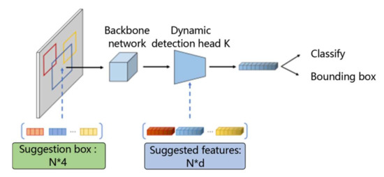
Figure 1.
Schematic diagram of a Sparse R-CNN network.
Sparse R-CNNs apply the set prediction loss to a fixed size set of predictions for classification and bounding box coordinates. The prediction loss is defined as follows:
where is the focus loss between the predicted target classification and the true label classification; and are the loss and generalized Intersection-over-Union (IoU) loss between the normalized center coordinates, height, and width of the predicted frame and the true bounding box; and , , and are the coefficients of the three losses, which are pre-defined hyper-parameters. The final loss of the model is the sum of all matched pairs after normalization based on the number of targets in the training batch.
Sparse R CNN-Based Vehicle Detection at Intersections
Vehicle detection at intersections is essentially an application of object detection algorithms in the traffic domain. Given the excellent performance of Sparse R-CNN on the publicly available datasets, we applied it to vehicle detection at intersections for obtaining the location and classification information of vehicles appearing in UAV images. The basic process is as follows: Firstly, a model is trained using training data so that the deep neural convolutional network can extract and classify the vehicle features in the image. Then, the features of the object vehicle area in the image are extracted by the network model, and these features with location attributes are input to the detection module for judgement. Finally, a bounding box of the vehicle that can be circled is produced, and the vehicle is classified.
After the vehicle detection image is input into Sparse R-CNN, a fixed number of learnable suggestion frames, which are randomly distributed over the image and basically cover the whole image, are initialized by the model, as shown in Figure 2a. Sparse R-CNN gradually refines the location of the target bounding box through the iterative module while removing duplicate bounding box locations. Finally, the model outputs accurate vehicle positioning bounding box and classification information, as shown in Figure 2b.
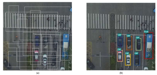
Figure 2.
Schematic diagram of the vehicle prediction frame at different stages in the Sparse R-CNN. (a) Learnable suggestion box. (b) Results.
Based on this training model, the video image sequences are processed to provide accurate vehicle location information data for subsequent vehicle object and trajectory extraction, while vehicle bounding box information can also be output to provide effective vehicle size information for the subsequent conflict indicator considering vehicle size.
3.2. Vehicle Trajectory Extraction Algorithm
The detection algorithm processes the vehicle detection results of each frame in the complete video image sequence. Due to the short time interval between frames (0.03 s) and the slow speed of most vehicles driving at road intersections, there must be a relatively high overlap between the bounding boxes of two adjacent frames for each vehicle. This overlap can be measured using the IoU ratio.
As shown in Figure 3, the IoU ratio is the ratio of the area of the intersection of two regions to the area of the concatenation of two regions and is calculated as shown in Equation (2).
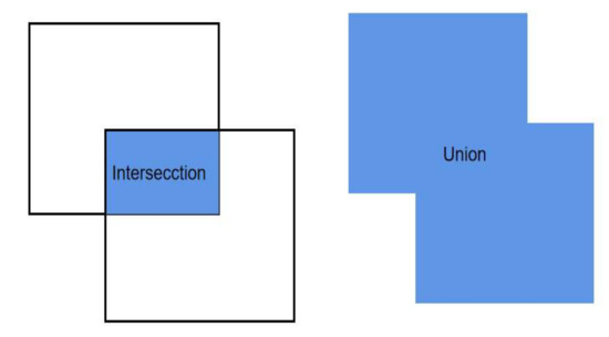
Figure 3.
Schematic diagram of the intersection and merging of two regions.
A trajectory extraction method is used to create a tracker for each object (vehicle in a specific area of the video). The position of the vehicle predicted by each tracker in the next frame and the result of the vehicle detection algorithm in the next frame are calculated separately. When the intersection ratio is greater than a set threshold, the bounding box generated by the detection algorithm can be assigned to the trajectory represented by the corresponding tracker. After the vehicle detection result is processed by the trajectory extraction algorithm, the trajectory information of each vehicle travelling at the road intersection during that time period can be obtained. The specific algorithm steps are given below and Figure 4 demonstrates the process of the vehicle trajectory extraction:
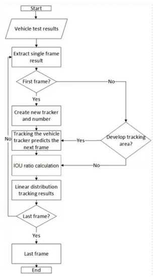
Figure 4.
Vehicle trajectory extraction algorithm.
- Read the video image sequence and the corresponding vehicle detection results.
- Extract the detection results of a single frame.
- If the frame is the first frame, initialize the tracker, that is, create and number the trackers for all the vehicles detected in the first frame of the video; if the frame is not the first frame, then only create and number the trackers for the vehicles located in the most tracked area (inlet or exit of the road intersection in all four directions).
- Update the tracker for each vehicle and make a bounding box prediction for the next frame.
- Obtain the detection results for the next frame and calculate the intersection ratio of each tracker's predicted bounding box to all the bounding boxes in the detection results separately and keep the results that meet the set threshold.
- Assign a corresponding detection result to each of the existing trackers using a linear assignment algorithm, that is, assign the result of the vehicle detection algorithm to the corresponding vehicle number.
- Return to Step 2 and cyclically execute the algorithm until the video sequence is processed.
4. Vehicle Conflict Indicator Metric Based on Improved Conflict Time Difference
Time difference to conflict includes four steps: vehicle speed and direction estimation, conflict distance computation, calculation of the TDTC indicator value, and threshold judgement.
4.1. The TDTC Calculation Method Applied to Vehicles at Intersections
When a UAV video is processed, the trajectory data of each vehicle can be obtained, that is, information about the position of each vehicle in each frame, which is generally represented by the coordinates of the vehicle in the image coordinate system. The position of a vehicle at a moment in time can be expressed as follows:
4.1.1. Time Difference to Conflict Considering Vehicle Size
Due to the large number of vehicle types at intersections, it is difficult to obtain the actual size of the vehicle based on the specific vehicle type. Therefore, the bounding box information (W,H) is used to approximate the size of each vehicle. W denotes the width of the bounding box of the vehicle and H denotes the length of the bounding box of the vehicle.
The TDTC was improved by considering the vehicle size factors mainly for two scenarios: rear-end conflict and crossover conflicts and lane change conflicts.
As shown in Figure 5, for a rear-end conflict considering the vehicle size factor, the expected conflict point is the contact point between the front vehicle and the rear vehicle at the time of collision. Combined with the geometric relationship in the image, it can be concluded that, for a rear-end conflict, a certain moment, set to is the front vehicle, and is the rear vehicle. Then, the two vehicles have zero between them, and the conflict is discriminated in the same way as the TTC indicator.
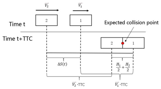
Figure 5.
Tailgating conflict considering vehicle size.
In Equations (4) and (5), is the distance of from the intersection at moment t; is the distance of from the intersection at moment t; is the velocity of at moment t; is the velocity of at moment t; and and are the lengths of the bounding boxes of vehicles and , respectively.
For crossover conflicts and lane change conflicts, if the vehicle is treated as a mass point, then the calculated TDTC actually represents the time difference between the respective center of the two vehicles moving at their current speed to the potential conflict point. If the size of the vehicle is considered, then the current potential conflict position of the conflicting vehicle cannot be considered to be a point but rather a potential conflict area approximating a circle. As shown in Figure 6, the dashed line in the diagram indicates the potential conflict state. For vehicle 1, the potential conflict area is the distance from vehicle 1’s position at that moment to the boundary of the potential conflict area if vehicle 2 is located at the intersection of the two vehicles' driving directions, and the potential conflict distance is the distance from vehicle 2’s position at the t moment to the boundary of the potential conflict area. The potential conflict distance is the distance from the position of vehicle 2 to the boundary of the potential conflict area at the moment.
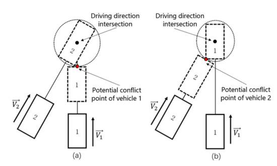
Figure 6.
Schematic diagram of a cross-conflict considering vehicle dimensions. (a) potential conflict point of vehicle 1, (b) potential conflict point of vehicle 2.
The smaller the time difference between the two vehicles arriving at the potential conflict zone, the more likely it is a conflict will occur. To accurately represent the time difference between the two vehicles at their respective current speeds until they reach the potential conflict point, the size of this potential conflict area is related to the size of the vehicle, and thus, when calculating the TDTC for and , the radius of the potential conflict area as well as its own vehicle length need to be subtracted from the distances and from the vehicle to the intersection point in the direction of speed. For crossover and lane change conflicts, the between the two vehicles at a given moment t when considering vehicle dimensions can be calculated as follows:
where is the distance of from the intersection at moment t; is the distance of from the intersection at moment t; is the velocity of at moment t; is the velocity of at moment t; and are the widths of the bounding boxes of vehicles and , respectively; and and are the lengths of the bounding boxes of vehicles and , respectively.
4.1.2. Calculation of the Vehicle Speed and Direction
As the time interval between each frame of the UAV video is very small, the vehicle can be regarded as making a uniform linear motion during this period from which the instantaneous velocity and direction of the vehicle can be calculated for the momentary frame, and the calculation formula is as follows:
where represents the distance that the vehicle moves from moment to moment ; and represents the angle between the velocity direction and the positive direction of the x-axis in the image coordinate system, which is used to represent the direction of the vehicle's movement at the t moment.
4.1.3. Calculation of the Potential Conflict Distance of a Vehicle
The potential conflict distance of a vehicle refers to the distance from the vehicle's location at the current t moment to the potential conflict area. The intersection points in the current direction of travel of the two vehicles are calculated first, and the intersection points that meet the conditions (i.e., the potential conflict points) are screened out. On this basis, the potential conflict distance of the vehicle is calculated by considering the vehicle size.
To calculate the intersection of the direction of travel at the t moment of the two vehicles, in the image coordinate system x–y, the equation for the line in which the direction of velocity of the two vehicles lies is derived as follows:
Then, using the method of solving for the intersection of two straight lines, the coordinates of the intersection point of the two vehicles in the direction of travel are derived from the joint solution. Like the method above, solving for the intersection of two straight lines can lead to situations where the solved intersection is not the intersection of the direction of travel. Additional judgement conditions need to be added to eliminate intersections that do not match. This is achieved by calculating whether or not the direction of the vector of two vehicles is the same as the direction of their own speed. The coordinates of the intersection of the two lines are found, and the two vectors and can be respectively calculated by
where and respectively represent the angle between the direction of speed of the two vehicles and the direction of the vehicles to the intersection point. The calculated intersection point is the direction of travel intersection. When the direction of travel intersection is calculated, the distances of the two vehicles from the direction of travel intersection can be calculated according to the distance formula.
4.1.4. Time Difference to Conflict Calculation and Threshold Determination
Combining the above, once the respective potential conflict distances of the two vehicles have been calculated, the conflict time difference TDTC values for the t moment vehicles and can be calculated by bringing Equations (4), (5), (7), (19), and (20) into Equation (6).
With reference to the threshold value of the intersection TTC indicator, it is set so that when the absolute value of TDTC is less than 1.5 s, the two vehicles are judged to be in conflict at the current moment. As a conflict is a continuous process, theoretically, if vehicles A and B have clashed, then they should be judged by the model to have clashed in several successive frames of the video (several successive moments). Therefore, to reduce misjudgment and improve the accuracy of conflict indicator, it is set only when the number of moments in which the two vehicles are judged to have clashed is greater than five.
5. Experiments
5.1. Experimental Data
Dataset
We chose five road sections with high traffic flow and collected traffic video using the INSPIRE 1 Pro UAV manufactured by DJI with a video frame rate of 30 frames per second. The position of the drone during filming is shown in Figure 7, with the filming angle perpendicular to the road surface. This filming method could capture the global information of the intersection with relatively few dead ends, making the collected data more conducive to vehicle detection and identification and conflict indicators. The hovering height of the drone was 126 m, and the main parameters of the traffic video data collection are shown in Table 1. The datasets are generated from 10 video segments from five urban road intersections.
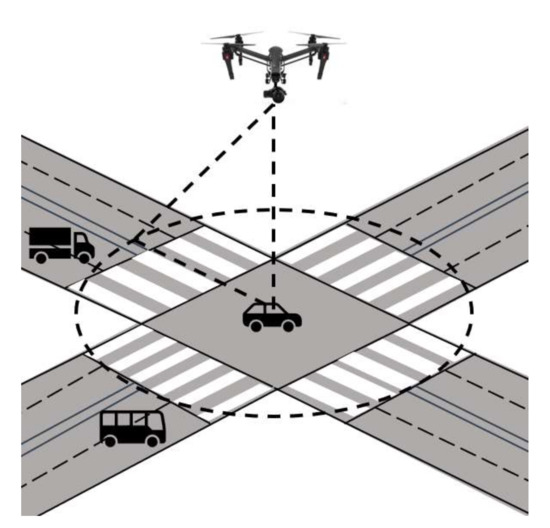
Figure 7.
Diagram of the location of the drone shot.

Table 1.
Traffic video capturing parameters.
The captured video data were pre-processed, mainly to correct the UAV video, and we used Fourier Merlin transform [42] to correct the video. The original 4k images were divided into a number of sub-images of uniform size in the order of top to bottom and left to right, with the sub-images having a size of 256 pixels overlapping the neighboring sub-images. Since the width of the original images was 2160 pixels, which cannot be divided by 256, the segmentation of the sub-images at the lower border of the image was achieved by starting at the lower border and going 512 pixels upwards.
Given the sub-images, the object vehicles in the sub-images needed to be annotated. We classified vehicles into bus, car, and truck types and annotated the vehicles in the image in the form of rectangular bounding boxes. The statistical results of the three types of vehicles in the dataset are shown in Table 2. The training and test datasets were divided randomly, and the statistics of the number of the three types of vehicles after the division are shown in Table 3.
Table 2.
Statistical results of the three types of vehicles in the collected datasets. RS represents the different road intersections.
Table 3.
Statistical result of the three vehicles in the training and test sets.
5.2. Vehicle Detection Experiments
5.2.1. Setup
The hyperparameters of the three models were configured in the model configuration file, with ResNet-50 [43] as the backbone network, and initialized using the pre-training weights obtained from ImageNet [44]. The optimization method used AdamW, with weights decaying by 0.0001. Since a single graphics card was used for training, the batch size was set to 16, and the maximum number of iterations was set to 270,000, where the initial learning rate of Sparse R-CNN was set to 0.000025 for better training results. Data enhancement methods included resizing the input image, random horizontal flipping, and scaling dithering.
The hyperparameters in the Sparse R-CNN loss function Equation (1) and were set to 2, and was set to 5. The default numbers were used for the suggested frames. The suggested features and corresponding iterations were 100, 100, and 6.
5.2.2. Evaluation Metrics
The object detection algorithm uses the IoU metric to measure the degree of similarity between the object bounding box predicted by the model and the true bounding box. The IoU is defined and calculated as described in Section 3.2. of this paper. The following are some of the relevant metrics and concepts used to evaluate the model.
The ground truth (GT) denotes the boundary frame and classification of a real existing vehicle in an image, obtained by manual annotation; true positive (TP) denotes the number of detected frames whose IoU with GT was greater than the set threshold, and the same GT was only calculated once; false positive (FP) denotes the number of detected frames whose IoU with GT were less than or equal to the set threshold or the number of redundant detected frames with the same GT detected; and false negative (FN) denotes the number of detected frames with no GT detected.
Precision accuracy, that is, the accuracy rate, represents the proportion of real vehicles in the results marked as vehicles, and it is calculated as follows:
The recall represents the proportion of correctly identified vehicles to all real vehicles, and it is calculated as follows:
The F1-score equilibrium average is calculated by combining the model accuracy and detection rates as follows:
Average precision (AP), which is a measure of the model's detection accuracy for each category, is calculated by averaging the precision over a precision–recall (PR) curve. For the PR curve, the calculation is performed using an integral with the following equation:
In practice, however, the AP is not calculated based on the original PR curve but rather on the PR curve after a smoothing operation has been performed. The specific way in which the curve is smoothed is that the value of precision at each point on the curve is taken to be the value of the largest precision to the right of that point.
The above formula is used to calculate the value of AP. Here, AP50 is the AP value at an IoU threshold of 0.5, and AP75 is the AP value at an IoU threshold of 0.75. The mean average precision (mAP) is the average of all the AP categories.
5.2.3. Model Training Results
In this paper, three deep neural networks, Sparse R-CNN, Faster R-CNN, and RetinaNet, as well as YOLO, were trained separately. Due to the performance limitation of the training equipment, the training took a longer time, and the time required for training the three networks as well as the detection speed on the test set are shown in Table 4. After completing the training, the final model vehicle detection was tested on the test dataset, and the evaluation metrics for the four networks are shown in Table 5.
Table 4.
Model training time and detection speed.
Table 5.
The comparison of four models on the vehicle detection performance.
Table 5 shows that Sparse R-CNN achieved the best results, with an mAP reaching 76.27% and AP50 and AP75 reaching 96.89% and 93.46%, respectively. Both were higher than those of Faster R-CNN, RetinaNet, and YOLO. Besides, R-CNN and RetinaNet were much closer, with 72.47% and 71.79% for their mAP, 90.12% and 90.15% for AP50, and 88.9% and 88.84% for AP75, respectively. YOLO achieved a slightly better performance than the Faster R-CNN and RetinaNet but performed worse than Sparse-RCNN with a 3% decrease. Although Sparse R-CNN required a longer training time, it could improve its average accuracy by about 5% with vehicle detection speeds similar to Faster R-CNN and RetinaNet. Taken together, the Sparse R-CNN model can be used for vehicle detection and the recognition of UAV video data to obtain better results and provide a better data base for subsequent trajectory extraction and vehicle conflict indicators.
5.2.4. Comparison of the Actual Detection Effect of the Models
To test the actual intersection vehicle detection effect of the three vehicle detection models, Sparse R-CNN, Faster R-CNN, and RetinaNet, five 4k resolution images were selected from five traffic videos taken with high traffic flow, and five 4k resolution images were obtained as test data to compare the detection effects of the three vehicle detection models. The precision detection rate, recall detection rate, and F1-score (see Section 5.2.2) were used to evaluate the three vehicle detection models, where TP is the number of vehicles detected correctly, FP is the number of objects detected incorrectly as vehicles, and FN is the number of vehicles that were not detected. The statistics of the detection results for the three models are given in Table 6, Table 7, Table 8 and Table 9.
Table 6.
Sparse R-CNN model detection results.
Table 7.
Faster R-CNN model detection results.
Table 8.
RetinaNet model detection results.
Table 9.
Comparison of accuracy of three models.
By analyzing the data in the above table, it can be found that the actual vehicle detection results of the three detection models are in line with the evaluation of the training results of the models in Table 5, in which Sparse R-CNN had a better overall effect. When the three vehicle detection models are analyzed in detail, the Sparse R-CNN had the best results for the “Car” and “Truck” types of vehicles, as well as the “Bus” type of vehicle, with fewer false detections. Faster R-CNN had the best results for “Car” and “Truck” vehicles, with fewer false detections. However, there were more false detections for “Bus.” Faster R-CNN and RetinaNet performed similarly, with the former detecting “Car” vehicles better than the latter, and the latter detecting “Truck” vehicles slightly better. The main reason for this is that the background color in some scenes near the road was too close to the color scheme of some buses (blue and white), which led to an increase in FPs. Moreover, in some scenarios, the container trucks were longer than other types of vehicles, which made it more difficult for the model to identify them, and there were also FPs due to the similar background color of the “Bus” type of vehicle. None of the three models were effective in detecting the “Truck” type. The Sparse R-CNN was more accurate and effective than the other two networks, and thus it is used as the vehicle detection algorithm.
5.3. Experiments of Vehicle Trajectory Extraction
Comparison of Different Trajectory Extraction Algorithms
To verify the effectiveness of the proposed vehicle trajectory extraction method, three other commonly used object tracking algorithms, MIL, KCF, and CSRT, were compared.
Firstly, a vehicle was randomly selected as the object vehicle in the UAV video, and the position information of the object vehicle in each frame was obtained by manual marking. Then, the real trajectory information of the vehicle was obtained over a period of time. At the same time, the vehicle trajectory extraction method was proposed, and three other object algorithms were used to process the tracked vehicle and output the trajectory results, and the trajectory extraction effect of the different algorithms was evaluated by calculating the difference between the trajectory points generated by the four algorithms and the real trajectory points. The gap between the trajectory points output by the algorithms and the real trajectory points was expressed using the distance between two points, which was calculated formulas follows:
where denotes the track point generated by the object algorithm, the coordinates are denoted by denotes the real track point of the tracked vehicle, and the coordinates are denoted by . During the experiment, the error (distance) between the tracked track points and the real track points in each frame was counted and plotted on a line graph, and, finally, the total error of all frames and the average error of each frame were calculated.
The results of the object experiments for the four algorithms are shown in Table 10 and Figure 8. The tracked vehicles selected in the experiments experienced a total of 297 frames in the video. The vehicle object and trajectory extraction algorithm proposed based on the vehicle detection model performed the best among the four algorithms, with an average error of about 1 pixel per frame. The error line graph shows that, although the error was larger in individual frames, the overall error variation trend was more stable compared to the other three object algorithms. This shows that the vehicle object and trajectory extraction algorithm used is more effective than the traditional object algorithm.
Table 10.
Error value statistics for four vehicle trajectory extraction algorithms.
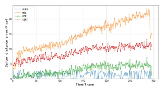
Figure 8.
Error comparison of the four vehicle trajectory extraction algorithms.
5.4. Time Difference to Conflict Conflict Indicator Index Comparison
To evaluate the effectiveness of the conflict indicator based on the improved TDTC metrics proposed and to avoid the influence of the accumulated errors in the vehicle detection and trajectory extraction stages on the evaluation results, some conflict vehicle samples from the traffic video were selected, and manual annotation was used to obtain the real trajectory information of the conflict samples to establish the conflict vehicle trajectory data set. Experiments were conducted to evaluate the conflict indicator effect of the improved TDTC metrics while comparing the unimproved TDTC metrics.
5.4.1. Experimental Results and Analysis
Experimental Results
The sample data was input into the TDTC indicator conflict indicator model based on the vehicle size improvement proposed, and the output results are shown in Table 11. The model used the interval of two frames to obtain the front and rear positions of the vehicles and calculate the speed. For 150 frames, if the number of frames in which a conflict was detected was greater than five, then the two vehicles were judged to be in conflict.
Table 11.
Conflict indicator results based on the improved TDTC metrics.
From the calculation of the relevant metrics in Section 5.2.2 combined with the data in Table 12, it can be concluded that, using the sample data, the conflict indicator model based on the improved TDTC metrics had 86% accuracy, 87.3% precision, 92.5% recall, and the equilibrium mean F1-score value was 89.9%.
Table 12.
Comparison of model results considering and not considering vehicle size factors.
Difference in Results between Considering and Not Considering Vehicle Size
The results of the experiments considering and not considering vehicle size are shown in Table 12, given that the other pre-set parameters in the model were the same.
As shown in Table 12, the accuracy of the vehicle conflict indicator for the sample data was improved when vehicle size was factored into the TDTC metrics, although the accuracy rate was reduced. The recall and F1-score were improved compared to the TDTC metrics without vehicle size factored in. This shows that the vehicle size factor is a necessary consideration for the identification of conflicts between vehicles at intersections with dense traffic flow and complex vehicle types, and it has a significant effect on improving the conflict indicator accuracy.
5.5. Vehicle Conflict Detection Based on Sparse R-CNN with Improved TDTC Metrics
Comprehensive Experiments
Based on the results of the vehicle detection model comparison experiments in Section 5.2 and the improved TDTC metrics comparison experiments in Section 5.4, the Sparse R-CNN model was selected as the vehicle identification algorithm in the vehicle detection phase, and the improved TDTC metrics based on vehicle dimensions were selected as the conflict indicator metrics in the vehicle conflict detection phase. To evaluate the conflict recognition effect of the method proposed in the text, the sample data selected in Section 5.4 were used as the validation data. The vehicle detection and trajectory extraction processes were carried out for all the videos where the sample vehicles were located. Then, the trajectory information of the corresponding time periods of the sample vehicles was obtained in the results, and the trajectory information of each sample vehicle was input into the conflict indicator model based on the improved conflict time difference indicator to output the results. Finally, in addition, this study also compared the conflict indicator effect based on two other vehicle detection models to verify the influence of the vehicle detection model on the conflict indicator effect of the final model. The experimental results are given in Table 13.
Table 13.
Comparison of conflict indicator results based on three vehicle detection models.
Table 13 shows that the accuracy and recall as well as the equilibrium mean of conflict indicator based on Sparse R-CNN and improved TDTC were the highest among the three models, while the check-all rates of the conflict indicator models based on RetinaNet and Faster R-CNN were both higher than that of Sparse R-CNN. Analyzing the confusion matrix shows that RetinaNet and Faster R-CNN were better than Sparse R-CNN in discriminating non-conflicted data. However, both were worse than Sparse R-CNN in discriminating conflicting samples, and thus Sparse R-CNN had the highest equilibrium mean. Overall, it can be proved that using Sparse R-CNN with a higher vehicle detection accuracy can improve the accuracy of the final vehicle conflict indicator, and the comprehensive conflict indicator is better.
6. Conclusions
In this paper, an automatic vehicle conflict recognition framework using deep learning and conflict time difference was proposed. Comprehensive experiments demonstrated the superiority and adaptability of the proposed method. Sparse R-CNN was adopted for vehicle detection, and it outperformed the other types of deep neural network object detection models. Given the vehicle detection, this paper implemented a vehicle trajectory extraction algorithm based on the overlap of the same vehicles. Compared with traditional semi-automatic object algorithms such as MIL, KCF, and CSRT, the proposed algorithm can achieve multiple vehicle tracking and trajectory extraction. The experimental results show that the proposed method obtained better trajectory.
Besides, we improve the TDTC metrics for vehicle conflict recognition by considering vehicle size for different types of conflicts. The real experimental results show that it could identify vehicle conflicts more accurately, and the discrimination accuracy was significantly improved compared with a metric that did not consider the vehicle size factor.
One of the drawbacks is that the proposed method relies on the sparse RCNN for vehicle detection, which has high requirements for computation resources. Finding the lightweight object detection models such as YOLOv5 that run in common computers is a promising direction.
Author Contributions
Conceptualization, Q.L. and Z.L.; methodology, Q.L., J.C.; software, J.C.; validation, Z.L., T.M.; formal analysis, Q.L., J.Z.; investigation, Z.L.; resources, J.Z.; data curation, Z.L., J.C.; writing—original draft preparation, Q.L., Z.L.; writing—review and editing, Q.L., J.Z.; visualization, J.C., Z.L.; supervision, J.Z.; project administration, J.Z.; funding acquisition, J.Z. All authors have read and agreed to the published version of the manuscript.
Funding
This research was funded by National Natural Science Foundation of China under Grant 41871329 and in part by the Science and Technology Planning Project of Guangdong Province under Grant 2018B020207005.
Institutional Review Board Statement
Not applicable.
Informed Consent Statement
Not applicable.
Acknowledgments
We thank all the reviewers and editors for their work in reviewing the paper.
Conflicts of Interest
The authors declare no conflict of interest.
References
- Tageldin, A.; Sayed, T. Developing evasive action-based indicators for identifying pedestrian conflicts in less organized traffic environ ents. J. Adv. Transp. 2016, 50, 1193–1208. [Google Scholar] [CrossRef]
- Wang, D.; Wu, C.; Li, C.; Zou, Y.; Zou, Y.; Li, K. Design of Vehicle Accident Alarm System for Sudden Traffic Accidents. World Sci. Res. J. 2021, 7, 169–175. [Google Scholar]
- Qi, Y.G.; Brian, L.; Guo, S.J. Freeway Accident Likelihood Prediction Using a Panel Data Analysis Approach. J. Transp. Eng. 2007, 133, 149–156. [Google Scholar] [CrossRef]
- Fu, C.; Sayed, T.; Zheng, L. Multi-type Bayesian hierarchical modeling of traffic conflict extremes for crash estimation. Accid. Anal. Prev. 2021, 160, 106309. [Google Scholar] [CrossRef] [PubMed]
- Uzondu, C.; Jamson, S.; Lai, F. Exploratory study involving observation of traffic behaviour and conflicts in Nigeria using the Traffic Conflict Technique. Saf. Sci. 2018, 110, 273–284. [Google Scholar] [CrossRef]
- Vuong, T.Q. Traffic Conflict Technique Development for Traffic Safety Evaluation under Mixed Traffic Conditions of Developing Countries. J. Traffic Transp. Eng. 2017, 5, 228–235. [Google Scholar]
- Olszewski, P.; Osińska, B.; Szagała, P.; Włodarek, P.; Niesen, S.; Kidholm, O.; Madsen, T.; Van Haperen, W.; Johnsson, C.; Laureshyn, A.; et al. Review of Current Study Methods for VRU Safety. Part 1–Main Report; University of Technology: Warsaw, Poland, 2016. [Google Scholar]
- Hayward, J.C. Near miss determination through use of a scale of danger. In Proceedings of the 51 Annual Meeting of the Highway Research Board, Washington, DC, USA, 17–21 January 1972; pp. 24–34. [Google Scholar]
- Cooper, P.J. Experience with Traffic Conflicts in Canada with Emphasis on Post Encroachment Time Techniques. International Calibration Study of Traffic Conflict Techniques; Springer: Berlin/Heidelberg, Germany, 1984; pp. 75–96. [Google Scholar]
- Cooper, D.; Ferguson, N. A Conflict simulation model. Traffic Eng. Control 1976, 17, 306–309. [Google Scholar]
- Golakiya, H.D.; Chauhan, R.; Dhamaniya, A. Mapping Pedestrian-Vehicle Behavior at Urban Undesignated Mid-Block Crossings under Mixed Traffic Environment—A Trajectory-Based Approach. Transp. Res. Proc. 2020, 48, 1263–1277. [Google Scholar] [CrossRef]
- Zhao, C.; Zheng, H.; Sun, Y.; Liu, B.; Zhou, Y.; Liu, Y.; Zheng, X. Fabrication of Tannin-Based Dithiocarbamate Biosorbent and Its Application for Ni(II) Ion Removal. Water Air Soil Pollut. 2017, 228, 1–15. [Google Scholar] [CrossRef]
- Rifai, M.; Budiman, R.A.; Sutrisno, I.; Khumaidi, A.; Ardhana, V.Y.P.; Rosika, H.; Tibyani Setiyono, M.; Muhammad, F.; Rusmin, M.; Fahrizal, A. Dynamic time distribution system monitoring on traffic light using image processing and convolutional neural network method. IOP Conf. Ser. Mater. Sci. Eng. 2021, 1175, 012005. [Google Scholar] [CrossRef]
- Cao, N.; Huo, W.; Lin, T.; Wu, G. Application of convolutional neural networks and image processing algorithms based on traffic video in vehicle taillight detection. Int. J. Sens. Netw. 2021, 35, 181–192. [Google Scholar] [CrossRef]
- Bautista, C.M.; Dy, C.A.; Manalac, M.I.; Orbe, R.A.; Cordel, M. Convolutional Neural Network for Vehicle Detection in Low Resolution Traffic Videos. In Proceedings of the 2016 IEEE Region 10 Symposium (TENSYMP), Bali, Indonesia, 9–11 May 2016; pp. 277–281. [Google Scholar]
- Redmon, J.; Divvala, S.; Girshick, R.; Farhadi, A. You Only Look Once: Unified, Real-Time Object Detection. In Proceedings of the IEEE Conference on Computer Vision and Pattern Recognition, Las Vegas, NV, USA, 27–30 June 2016; pp. 779–788. [Google Scholar]
- Bochkovskiy, A.; Wang, C.; Liao, H.M. YOLOv4: Optimal Speed and Accuracy of Object Detection. arXiv 2020, arXiv:2004.10934. [Google Scholar]
- Girshick, R.; Donahue, J.; Darrell, T.; Malik, J. Rich feature hierarchies for accurate object detection and semantic segmentation. In Proceedings of the 2014 IEEE Conference on Computer Vision and Pattern Recognition, Columbus, OH, USA, 23–28 June 2014; pp. 580–587. [Google Scholar]
- Girshick, R. Fast r-cnn. In Proceedings of the IEEE International Conference on Computer Vision, Boston, MA, USA, 7–12 June 2015; pp. 1440–1448. [Google Scholar]
- Ren, S.; He, K.; Girshick, R.; Sun, J. Faster R-CNN: Towards Real-Time Object Detection with Region Proposal Networks. IEEE Trans. Pattern Anal. Mach. Intell. 2017, 39, 1137–1149. [Google Scholar] [CrossRef] [Green Version]
- Xu, Y.; Yu, G.; Wang, Y.; Wu, X. Car Detection from Low-Altitude UAV Imagery with the Faster R-CNN. J. Adv. Transp. 2017, 2017, 1–10. [Google Scholar] [CrossRef] [Green Version]
- Sun, P.; Zhang, R.; Jiang, Y.; Kong, T.; Xu, C.; Zhan, W.; Tomizuka, M.; Li, L.; Yuan, Z.; Wang, C.; et al. Sparse R-CNN: End-to-End Object Detection with Learnable Proposals. In Proceedings of the IEEE/CVF Conference on Computer Vision and Pattern Recognition, Nashville, TN, USA, 19–25 June 2021; pp. 14454–14463. [Google Scholar]
- Cao, J.; Zhang, J.; Jin, X. A Traffic-Sign Detection Algorithm Based on Improved Sparse R-cnn. IEEE Access 2021, 9, 122774–122788. [Google Scholar] [CrossRef]
- Uijlings, J.R.R.; van de Sande, K.E.A.; Gevers, T.; Smeulders, A.W.M. Selective Search for Object Recognition. Int. J. Comput. Vis. 2013, 104, 154–171. [Google Scholar] [CrossRef] [Green Version]
- Grabner, H.; Bischof, H. On-Line Boosting and Vision. In Proceedings of the Computer Society Conference on Computer Vision and Pattern Recognition, New York, NY, USA, 17–22 June 2006; pp. 260–267. [Google Scholar]
- Felzenszwalb, P.F.; Girshick, R.B.; McAllester, D.; Ramanan, D. Object Detection with Discriminatively Trained Part-Based Models. IEEE Trans. Pattern Anal. Mach. Intell. 2010, 32, 1627–1645. [Google Scholar] [CrossRef] [PubMed] [Green Version]
- Kalal, Z.; Mikolajczyk, K.; Matas, J. Tracking-Learning-Detection. IEEE Trans. Pattern Anal. Mach. Intell. 2012, 34, 1409–1422. [Google Scholar] [CrossRef] [Green Version]
- Lim, J.; Yang, M. Online Object Tracking: A Benchmark. In Proceedings of the 2013 IEEE Conference on Computer Vision and Pattern Recognition, Portland, OR, USA, 23–28 June 2013; pp. 2411–2418. [Google Scholar]
- Yun, S.; Choi, J.; Yoo, Y.; Yun, K. Action-Decision Networks for Visual object with Deep Reinforcement Learning. In Proceedings of the 2017 IEEE Conference on Computer Vision and Pattern Recognition, Honolulu, HI, USA, 22–25 July 2017; pp. 1349–1358. [Google Scholar]
- Fan, H.; Ling, H. Sanet: Structure-Aware Network for Visual object. In Proceedings of the 2017 IEEE Conference on Computer Vision and Pattern Recognition Workshops (CVPRW), Honolulu, HI, USA, 22–25 July 2017; pp. 2217–2224. [Google Scholar]
- Li, P.; Wang, D.; Wang, L.; Lu, H. Deep visual object: Review and experimental comparison. Pattern Recognition 2018, 76, 323–338. [Google Scholar] [CrossRef]
- Chen, Y.; Wang, J.; Xia, R.; Zhang, Q.; Cao, Z.; Yang, K. The visual object tracking algorithm research based on adaptive combination kernel. J. Ambient Intell. Humaniz. Comput. 2019, 10, 4855–4867. [Google Scholar] [CrossRef]
- Mahanta, G.B.; Rout, A.; Biswal, B.B.; Deepak, B.B.V.L. An improved multi-objective antlion optimization algorithm for the optimal design of the robotic gripper. J. Exp. Theor. Artif. Intell. 2020, 32, 309–338. [Google Scholar] [CrossRef]
- Ping, C.; Dan, Y. Improved Faster RCNN Approach for Vehicles and Pedestrian Detection. Int. Core J. Eng. 2020, 6, 119–124. [Google Scholar]
- Zheng, L.; Sayed, T. Bayesian hierarchical modeling of traffic conflict extremes for crash estimation: A non-stationary peak over threshold approach. Anal. Methods Accid. Res. 2019, 24, 100106. [Google Scholar] [CrossRef]
- Puri, A.; Valavanis, K.P.; Kontitsis, M. Statistical profile generation for traffic monitoring using real-time UAV based video data. In Proceedings of the 2007 Mediterranean Conference on Control & Automation, Athens, Greece, 27–29 June 2007; pp. 1–6. [Google Scholar]
- Meng, X.H.; Zhang, Z.Z.; Shi, Y.Y. Research on Traffic Safety on Freeway Merging Sections Based on TTC and PET. Appl. Mech. Mater. 2014, 587, 2224–2229. [Google Scholar] [CrossRef]
- Jiang, R.; Zhu, S.; Wang, P.; Chen, Q.; Zou, H.; Kuang, S.; Cheng, Z. In Search of the Consequence Severity of Traffic Conflict. J. Adv. Transp. 2020, 2020, 9089817. [Google Scholar] [CrossRef]
- St-Aubin, P.; Saunier, N.; Miranda-Moreno, L. Large-scale automated proactive road safety analysis using video data. Transp. Res. Part C 2015, 58, 363–379. [Google Scholar] [CrossRef]
- Charly, A.; Mathew, T.V. Estimation of traffic conflicts using precise lateral position and width of vehicles for safety assessment. Accid. Anal. Prev. 2019, 132, 105264. [Google Scholar] [CrossRef] [PubMed]
- Goecke, R.; Asthana, A.; Pettersson, N.; Pettersson, L. Visual vehicle egomotion estimation using the fourier-mellin transform. In Proceedings of the 2007 IEEE Intelligent Vehicles Symposium, Istanbul, Turkey, 13–15 June 2007; pp. 450–455. [Google Scholar]
- He, K.; Zhang, X.; Ren, S.; Sun, J. Deep residual learning for image recognition. In Proceedings of the IEEE Conference on Computer Vision and Pattern Recognition, Las Vegas, NV, USA, 27–30 June 2016; pp. 770–778. [Google Scholar]
- Krizhevsky, A.; Sutskever, I.; Hinton, G.E. Imagenet Classification with Deep Convolutional Neural Networks. Adv. Neural Inf. Process. Syst. 2012, 25, 1097–1105. [Google Scholar] [CrossRef]
- Yaodong, W.; Yuren, C. A Method of Identifying Serious Conflicts of Motor and Non-motor Vehicles during Passing Maneuvers. J. Transp. Inform. Safety 2015, 4, 61–68. [Google Scholar]
Publisher’s Note: MDPI stays neutral with regard to jurisdictional claims in published maps and institutional affiliations. |
© 2021 by the authors. Licensee MDPI, Basel, Switzerland. This article is an open access article distributed under the terms and conditions of the Creative Commons Attribution (CC BY) license (https://creativecommons.org/licenses/by/4.0/).