Assessment of Wildfire Activity Development Trends for Eastern Australia Using Multi-Sensor Earth Observation Data

Abstract

Increased fire activity across the Amazon, Australia, and even the Arctic regions has received wide recognition in the global media in recent years. Large-scale, long-term analyses are required to postulate if these incidents are merely peaks within the natural oscillation, or rather the consequence of a linearly rising trend. While extensive datasets are available to facilitate the investigation of the extent and frequency of wildfires, no means has been available to also study the severity of the burnings on a comparable scale. This is now possible through a dataset recently published by the German Aerospace Center (DLR). This study exploits the possibilities of this new dataset by exemplarily analyzing fire severity trends on the Australian East coast for the past 20 years. The analyzed data is based on 3503 tiles of the ESA Sentinel-3 OLCI instrument, extended by 9612 granules of the NASA MODIS MOD09/MYD09 product. Rising trends in fire severity could be found for the states of New South Wales and Victoria, which could be attributed mainly to developments in the temperate climate zone featuring hot summers without a dry season (Cfa). Within this climate zone, the ecological units featuring needleleaf and evergreen forest are found to be mainly responsible for the increasing trend development. The results show a general, statistically significant shift of fire activity towards the affection of more woody, ecologically valuable vegetation.

1. Introduction

Wildfires have always played a significant role in the evolution of various ecosystems and are the predominant natural disturbance factor in many parts of the world. They significantly influence ecological patterns and processes on a global scale. This includes vegetation distribution and structure, as well as the carbon cycle [1]. While humans and wildfires have always coexisted, changes in wildfire patterns represent an increasing threat to human lives and property. Apart from the direct implications, wildfires have also been found to contribute to the greenhouse effect through CO₂ emissions, thus fostering atmospheric changes on a global level [2,3]. Research has shown that forest loss has increased substantially over the past two decades in many parts of the world, and that the underlying dynamics are strongly linked to fire activity [4]. Several studies have discovered changes in the frequency and size of wildfires and also in the length of the fire season, for example, regarding the Canadian boreal forest [5] and the Western United States [6].

In recent years, large wildfires have occurred in regions formerly unaffected by fire, such as the Arctic regions. Some regions regularly affected by fire have experienced unprecedented large-scale fire events, such as the Australian East coast, the Brazilian Amazonas region, or the state of California in the United States. Investigating the question if these recent events are part of a natural oscillation, or must instead be regarded as a result of a long-term trend, is a crucial task in fire science. Studies usually analyze parameters such as the frequency of occurrence, spatial extent, and burn severity of fire incidents to derive meaningful trends [7].

To obtain insights regarding shifts in global fire activity, studies have to incorporate multi-decadal time spans and continental-scale study areas. Global, long-term burnt area datasets are readily available for analyses, the most widely used ones being the National Aeronautics and Space Administration (NASA) MCD64A1 dataset [8] and the European Space Agency (ESA) Fire_cci BA 5.1 dataset [9,10]. A third global burnt area product from the Global Fire Emissions Database, version 4 (GFED4, [11]) is meanwhile discontinued and is only available until 2015 [12]. A semi-automatically generated product is also provided by the Joint Research Center of the European Commission (JRC) in the frame of the European Forest Fire Information System (EFFIS) [13]. However, these data are only available for Europe, Northern Africa, and the Middle East [14].

While the listed datasets all include the fire perimeter as well as the burning detection date, they do not feature information regarding the fire severity, and thus do not allow the derivation of trends in this regard. Yet, fire severity is a critical aspect of fire regimes, determining fire impacts on ecosystem attributes and associated post-fire recovery [15].

The German Aerospace Center (DLR) recently published a global, long-term burnt area dataset, which includes information regarding the burn severity, together with fire perimeter and the burning date. This dataset is closely linked to the burnt area monitoring service operated by DLR. It is maintained by the Department of Geo-Risks and Civil Security (GZS) of the German Remote Sensing Data Center (DFD). The service is based on mid-resolution Sentinel-3 Ocean and Land Color Instrument (OLCI) satellite imagery and provides burnt area information for the region of Europe twice a day in near-realtime. The service is fully automated and targeted at supporting rapid mapping activities and timely post fire damage assessment throughout Europe. A quality-optimized version called fusion product is generated after a time delay of 10 days, when additional post-event data is available.

The recently published, global dataset is build upon this fusion product. In addition to the data available for Europe, equivalent products are generated using the same methodology for North and South America, Africa, Oceania, and Asia. The methodology is briefly described consecutively, the complete description can be found in Nolde et al. [16]. As the dataset is based on Sentinel-3 data, it is only available since 2016, which is the year the first Sentinel 3 satellite was launched. For this study, the data was extended using data from the NASA MODIS MOD09/MYD09 product [17] in order to allow the derivation of trends on a longer time scale.

The complete input dataset comprises 9612 granules of the MODIS MOD09/MYD09 product in conjunction with 3503 tiles of the OLCI instrument onboard the Sentinel-3 satellite. The area of Eastern Australia has been selected as a study region, covering the states and territories of Queensland, New South Wales, the Australian Capital Territory (ACT), and Victoria, respectively.

This study region is chosen because it experienced destructive burnings in the 2019/2020 fire season, and because it also was regularly affected by wildfires in recent decades.

The year 2019 was Australia’s warmest year on record so far, with significant heat waves occurring in January and December [18]. The national, average maximum temperature was as high as 43.6 °C, which is more than 1.8 °C above the long-term average [19]. In addition, 2019 has also been the driest year on record in Australia, caused by an extraordinary strong positive Indian Ocean Dipole [20]. The nationally-averaged rainfall was 40% below average, amounting to only 278 mm. As a consequence, the annual, cumulative Forest Fire Danger Index reached the highest values since the beginning of the national records in 1950 [18]. Three of the four investigated states and territories, namely, New South Wales, the ACT, and Victoria, reside in a temperate climate zone, with dryness conditions usually reaching moderate levels at most [21]. However, in 2019, these states experienced severe drought conditions, with New South Wales suffering the most severe conditions throughout Australia. These preconditions contributed significantly to the unprecedented fire activity in December 2019 and January 2020 [19].

This study analyses the existence of stable, wildfire related trends in this region, focusing on fire severity.

2. Materials and Methods

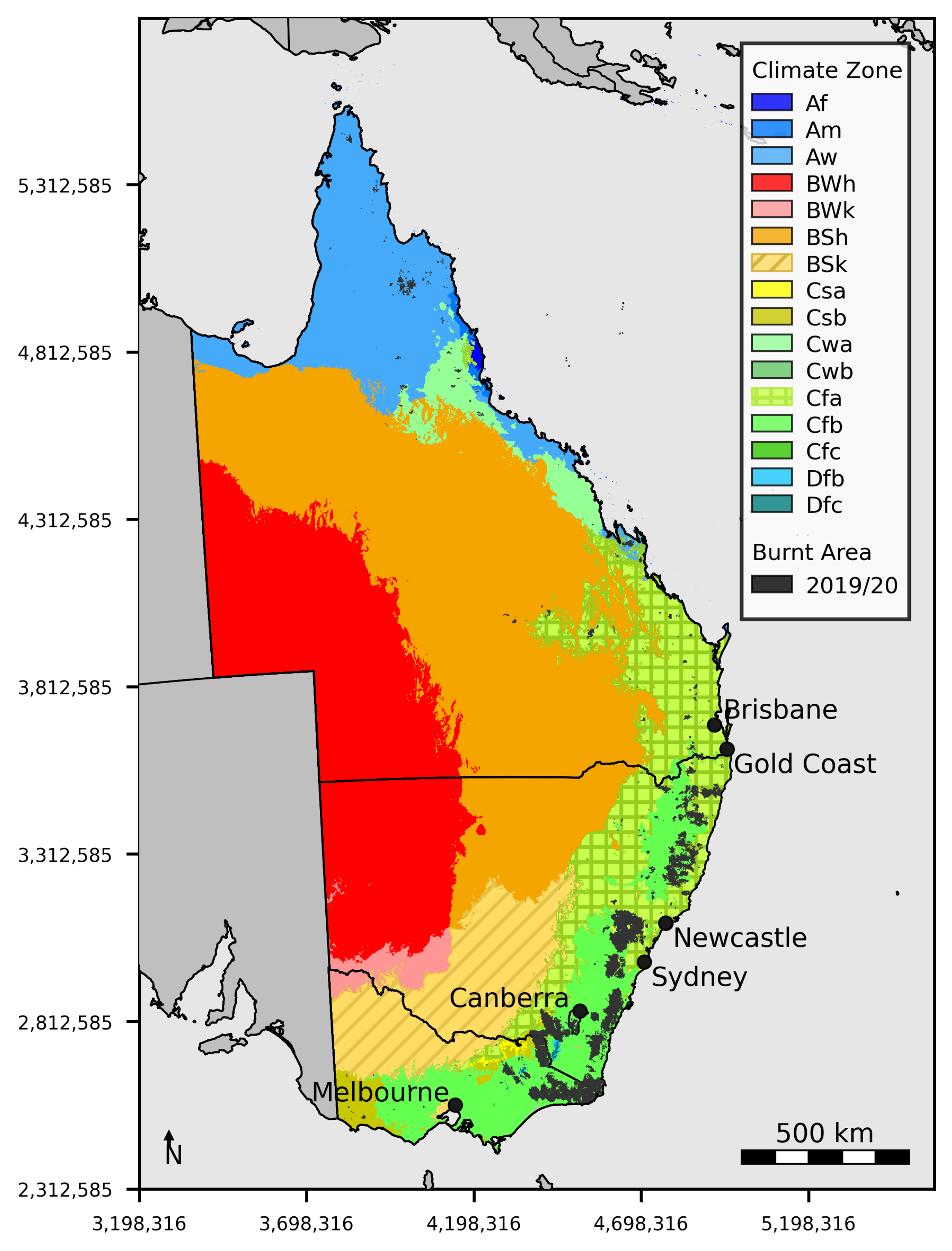
2.1. Area of Interest

The chosen study region comprises the states of Queensland, Victoria, and New South Wales together with the Australian Capital Territory (ACT). This region is vastly heterogeneous regarding climate and vegetation cover, with a pronounced inter-annual variability. Both Queensland and New South Wales include tropical, temperate, and arid climate zones. Figure 1 shows the area of interest, together with the respective climate zones and the burnt area from the 2019/2020 wildfire season. The highlighted climate zones are the ones found to feature increasing trends regarding fire severity in this study. The full names corresponding to the climate zone abbreviations can be found in the respective tables in the result section. This study is prepared in a hierarchical manner. Trends are analyzed on a state level, as well as regarding climate zones, and finally ecological units. These are consecutively set in relation to each other.

The utilized climate zone map, prepared by Beck et al. [22] following the methodology of Peel et al. [23], is derived using a long-term time series of weather station data regarding monthly precipitation and air temperature. The system classifies climatic regions into five main classes and 30 subtypes. The discrimination between classes is based on fixed thresholds addressing the seasonality of precipitation and temperature. Climate is recognized as the major driver of global vegetation. The classification is therefore regarded as an empirical mapping of biome distributions around the world. Although developed in the 19th century, it is widely used today, for example, in ecological modelling [22].

The Australian Forest Fire Danger Index [24] relies on four meteorological parameters, which have proven their reliability with regard to wildfire activity: temperature, wind speed, relative humidity, and the Drought Factor, a component representing fuel availability [25].

The latter parameter, which is strongly influenced by seasonal variations in rainfall, has been found to be pivotal for fire occurrence, together with the vegetation structure [26]. As described by Russel-Smith et al., fire frequency as well as fire extent throughout Australia are strongly influenced by rainfall seasonality. Fire occurrence is therefore most pronounced in the tropics of Northern Australia, which are intensely seasonal. Rainfall positively influences the dynamics of biomass growth, which provides the fuel for wildfire activity. Precipitation amounts above average could be attributed to large burnings in arid, central Australia [27].

Dryness, on the other hand, strongly increases the availability of the vegetation to burn [28]. It could be shown that drought conditions are associated with major fires in the forested areas of Southern Australia [29,30]. These ecosystems usually feature sufficient litter for propagation of fire at most times. The most influential factor for fire propagation is the availability of vegetation to burn, controlled by drought conditions and the weather at the time of ignition [28].

2.2. Utilized Data Sources

The study utilizes the DLR-GZS burnt area dataset, which is based on mid-resolution optical satellite data from two different sensors. First, the OLCI instrument onboard the Sentinel-3 A and B satellites of the European Copernicus Programme [31], and second, the MODIS instrument onboard the NASA Aqua/Terra satellites. Band information from the red and near-infrared (NIR) domain are utilized for the retrieval of burnt area perimeters and burn severity estimation. Imagery of the Sentinel-3 OLCI instrument can be retrieved via the Copernicus Open Access Hub [32] and the Copernicus online data access website [33]. However, the available time span for OLCI data is considerably shorter than the one regarding MODIS. Sentinel-3A was launched in 2016, with Sentinel-3B following in 2018. Therefore, the OLCI dataset is extended by imagery from the MODIS sensor for this study. This data is available for an extended time range of more than two decades, starting in late 1999 with the launch of the NASA Terra satellite. The sensor is designed to observe the ocean, atmosphere, land, and ice on the Earth’s surface [34]. It features 36 discrete spectral bands with differing spatial resolutions from 250 m to 1 km. Terra’s twin satellite, Aqua, was launched in 2002, carrying a second MODIS instrument. This study makes use of MODIS information provided through the MOD09A1/MYD09A1 surface reflectance product [17], which represents a cloud-free 8-day composite of bands in the visible spectrum. The data are freely available from the NASA Land Processes Distributed Active Archive Center (LP DAAC) [35]. Furthermore, thermal anomaly information derived from the MODIS MOD14A2/MYD14A2 [36] product is used as auxiliary data. Equivalent data is utilized from the Visible Infrared Imaging Radiometer Suite (VIIRS) instrument onboard the Suomi National Polar-orbiting Partnership (SUOMI-NPP) satellite [37]. Both products are available for download on the NASA Fire Information for Resource Management System (FIRMS) website [38].

In order to reduce the total data volume to a significant selection, only the Australian summer months from November to February have been analyzed in this study.

Subsequent to the derivation of burnt area perimeters and the burn severity, the results are combined with land use and land cover (LULC) data to gain insights regarding affected vegetation classes. For this purpose, the CCI-LC (Climate Change Initiative-Land Cover) product from ESA is used. It provides mid-resolution land cover information on a global scale. Moreover, land cover maps are available for each individual year, starting in 1992 [39]. To investigate the relationship between fire activity and climatic conditions, a climate zone map based on the Köppen-Geiger classification system is utilized, published by Beck et al., 2018 [22]. Furthermore, ecological units provided by the United States Geological Survey (USGS) are used [40].

Two further burnt area datasets have been incorporated within this study to validate the presented results. First, the NASA MCD64A1 dataset, featuring global burnt area information derived from MODIS imagery, with a spatial resolution of 500 m [8]. These data are made available by the University of Maryland [41] and has been widely utilized in academic research, for example, for the Brazilian Savannas [42,43]. Second, a high resolution burnt area map for the state of New South Wales is utilized, which was prepared by the Department of Planning, Industry and Environment of New South Wales/Australia. This dataset, named Google Earth Engine burnt area map (GEEBAM) [44], is based on Sentinel-2 data and makes use of manually derived thresholds from aerial photography [45]. The National Indicative Aggregated Fire Extent Datasets [46], which are published by the Australian Government, have also been taken into consideration as a reference data source. However, the GEEBAM dataset has been found to feature a higher thematic accuracy, and is therefore chosen as reference in this study.

Table 1. Analyzed data sources, listed separately for Queensland (QLD), New South Wales (NSW), Australian Capital Territory (ACT), and Victoria (VIC).

Time Span	Sensor	Scenes	Avg. Cloud-Free Overpasses per Pixel
			QLD	NSW	ACT	VIC
2000/11–2001/02	MODIS	240	10	13	13	14
2001/11–2002/02	MODIS	240	15	15	14	15
2002/11–2003/02	MODIS	480	30	30	27	30
2003/11–2004/02	MODIS	480	30	30	27	30
2004/11–2005/02	MODIS	480	28	29	26	28
2005/11–2006/02	MODIS	484	30	30	27	30
2006/11–2007/02	MODIS	480	30	30	27	30
2007/11–2008/02	MODIS	480	30	30	27	30
2008/11–2009/02	MODIS	480	28	29	26	28
2009/11–2010/02	MODIS	480	30	30	27	30
2010/11–2011/02	MODIS	480	30	30	27	30
2011/11–2012/02	MODIS	480	30	30	27	30
2012/11–2013/02	MODIS	480	28	29	26	28
2013/11–2014/02	MODIS	480	30	30	27	30
2014/11–2015/02	MODIS	488	30	30	27	30
2015/11–2016/02	MODIS	480	30	30	27	30
2016/11–2017/02	MODIS	480	28	29	26	28
	OLCI	620	33	45	36	34
2017/11–2018/02	MODIS	480	30	30	27	30
	OLCI	616	35	41	30	35
2018/11–2019/02	MODIS	480	30	30	27	30
	OLCI	1019	58	75	61	61
2019/11–2020/02	MODIS	480	28	29	26	28
	OLCI	1248	76	91	68	71

lists the complete set of available MOD09/MYD09 composites and Sentinel-3-OLCI scenes used for generating the DLR-GZS burnt area dataset, which this study is build upon. Besides the number of available scenes for each time range and state, the average number of cloud free observations per pixels is given, representing a measure of the interpretability of the data. As the MOD09/MYD09 data are available as an eight-day composite, the number of cloud-free observations is considerably lower when compared to Sentinel-3. In total, 9612 MODIS MOD09/MYD09 granules from both Terra and Aqua have been analyzed, together with 3503 OLCI scenes from Sentinel-3 A and B. This amounts to an entirety of 13,115 scenes for the complete study time span.

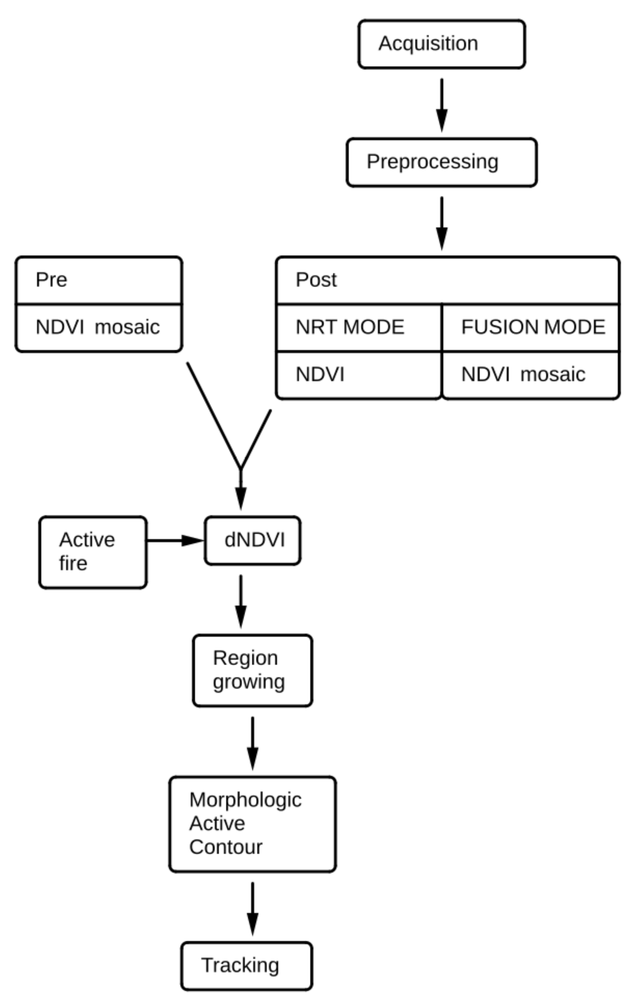
2.3. Burnt Area Derivation Methodology

The accurate, automatic monitoring of burnt area evolution from satellite imagery represents a demanding task for the scientific community. This is mostly due to the spatial-temporal variability of the state of the Earth’s surface. Inaccuracies are also introduced by the utilized sensor and related geometrical resolution [47]. Furthermore, the presence of clouds disturbs the derivation of meaningful surface features at reflective wavelengths [48]. Adding to the complexity inherent in optical sensor data, burnt areas are highly heterogeneous regarding size, shape, and spectral reflectance on the ground surface, and can thus be difficult to differentiate from shadows cast by clouds and mountains. These circumstances significantly limit the possibilities for an automated approach, especially on a large geographical scale. Many recent research activities have assessed these challenges using Machine Learning technologies. Methodologies such as Random Forests [49], Support Vector Machines [50], and Deep Learning classifiers [51,52] have been applied in this regard. However, research has mainly been focused on feature detection using high resolution satellite imagery on a small geographic scale. Due to the spatial resolution however, these satellites inherently feature a low temporal frequency, and are thus unsuited for daily monitoring purposes. Approaches utilizing mid-resolution satellite data, thus allowing a high temporal coverage for an extended geographical region, usually use a time series approach in combination with a burn-sensitive vegetation index. Thermal anomaly detections are often used as auxiliary data (see [53]). However, these approaches feature a significant amount of uncertainty. Humber et al. analyzed four global burnt area products, and concluded that the estimates of burned area vary greatly between products in terms of total area affected, the location of burning, and the timing of the burning [54]. In a similar study, Padilla et al. found that the commission error ratio was above 40% and omission error ratio was above 65% for the analyzed products [55]. Oliva et al. conducted a study investigating if thermal anomaly data could be used as a replacement for burnt area datasets, but found high omission and commission errors especially for grasslands, savannas, and agricultural areas [56].

The methodology utilized here is based on an approach developed at DLR [16]. It is primarily designed for monitoring continental-scale regions in near-real time, but can also be invoked to perform retrospective time series analysis. The derived information comprises burnt area perimeters, the date of detection, and the burn severity by means of the differential Normalized Difference Vegetation Index ($NDV{I}_{diff}$ [57], see Equations (1) and (2). As auxiliary information, the number of detections for each burnt area pixel is available, as well as the number of cloud-free satellite overpasses for each pixel.

$$NDVI=\frac{NIR-Red}{NIR+Red}$$

(1)

$$NDV{I}_{diff}=NDV{I}_{pre}-NDV{I}_{post}$$

(2)

At its core, the method exploits the synergetic effects of data from the red/NIR and the thermal wavelengths in order to derive burnt area information. Substantial work in this regard has been performed by Fraser et al. and Li et al. for the boreal forest of Canada as early as the year of 2000 [58,59].

As a basis for the processing, mosaics of pre- and post-$NDVI$ information are generated. Consecutively, the concept of Morphological Active Contours without Edges (MorphACWE [60,61]) is used to derive accurate burnt area perimeters. The method is closely related to Geodesic Active Contour Level Sets [62], which have been used for burnt area derivation [63] as well as other domains, such as crop field size estimation [64].

The term Active Contour refers to a dynamical curve, which grows starting from a set of seed pixels and converges when an optimal segmentation result is reached. For the generation of the burnt area dataset, Active Fire locations are used as seed information. This proceeding was shown to yield results of high geometric accuracy when inter-compared with the JRC/EFFIS dataset [13] as well as the NASA MCD64A1 dataset [8]. The accuracy validation, together with the detailed description of the methodology, can be found in Nolde et al. (2020) [16]. The methodology is schematically visualized in Figure 2.

Figure 3 shows exemplary visualizations of the data used for the preparation of this study. Sub-figure (a) visualizes the maximally detected burn severity regarding the mega fire in the greater area of Sydney/New South Wales, which was active during November and December, 2019. Sub-figure (b) shows the temporal evolution of the burn activity, by means of detection date.

2.4. Validation of Burnt Area Data

The presented results are compared against the two reference datasets, NASA MCD64A1 and GEEBAM, regarding three criteria:

• True positives (TP): The total burnt area contained in the presented results as well as the reference data, in relation to the total burnt area of the reference data.
• False negatives (FN): The total burnt area not contained in the presented results, but contained in the reference, in relation to the total burnt area of the reference data.
• False positives (FP): The total burnt area contained in the presented results, but not contained in the reference area, in relation to the total burnt area of the reference data.

The fourth criterion, which represents the true negatives (TN), refers to the percentage of area neither contained in the presented results, nor in the reference data. However, as the total size of unburnt area greatly predominates the total size of burnt area, this true negative percentage is implicitly very close to 100 percent. This is, however, mostly due to the size of the study region, so this measure does not represent a meaningful value for this kind of study. The same applies to the overall accuracy [65]. These measures have therefore been omitted in

Table 2. Inter-comparison of burnt area extent with NASA MCD64A1 and GEEBAM reference datasets.

		Presented Results 4,577,850 ha	MCD64A1 4,176,018 ha	GEEBAM 5,306,688 ha
presented results	TP	x	83.8%	77.1%
	FN	x	16.2%	22.9%
	FP	x	25.8%	9.2%
	TP/FPinv	x	79.0%	84.0%
MCD64A1	TP	76.4%	x	71.1%
	FN	23.6%	x	28.9%
	FP	14.8%	x	7.6%
	TP/FPinv	80.8%	x	81.7%
GEEBAM	TP	89.4%	90.3%	x
	FN	10.6%	9.7%	x
	FP	26.5%	36.8%	x
	TP/FPinv	81.4%	81.4%	x

, which shows the results of the evaluation. A more suited means of measure is to calculate the average of the true positive percentage and the inverted false positive percentage (false positives subtracted from 100%, named FP_inv in Table 2).

The inter-comparison of the burnt area of the presented results with the burnt area of the high resolution GEEBAM 2019/2020 data for New South Wales reveals a percentage of overlapping area of 77%, with an error of 9%. The Jaccard index, also known as Intersection over Union, yields a similarity of 70.8% [66]. To enable an evaluation of these numbers, the NASA MCD64A1 dataset is equivalently checked against the same reference, yielding 71% overlap and an error of 7%. The combination of true positives and inverted false negatives account for 84% for the presented results, and 82% for the MCD64A1 data. The results obtained in this study regarding the 2019/2020 fire season are in accordance with burnt area extent information published by Boer [67]. The data basis is therefore considered to be of satisfactory accuracy.

2.5. Trend Derivation Methodology

The trend derivation in this study is based on linear regression, whereby the slope of the regression line represents the actual trend. The input values for the burnt area extent analysis are the accumulated burnt area amounts per unit of investigation (state, climate zone, or ecological unit) for each year of the analyzed time span. Regarding the burn severity analysis, the input values are derived by averaging all values within the unit of investigation for each respective year. The correlation coefficient indicates to what extent the actual values are in concordance with the calculated trend line, while the RMSE (Root Mean Square Error) illustrates the error.

Finally, the 5- and 95-percentiles (named “Perc 5” and “Perc 95” in the result tables) represent the error margins, indicating how robust the result actually is. They are derived through repeatedly and randomly altering the input values within the range of the RMSE, so that the results reflect the average of a set of possible outcomes. To eliminate outliers, the 5 and 95-percentiles are used as upper and lower limits of the yielded results.

3. Results

The consecutive sub-sections show the results of the analysis on a state-wide level, as well regarding climatic zones and finally ecological units. These results are then set in relation to each other. Each subsection contains a visualization of the burnt area extent for each year within the analyzed time span, followed by the actual burn severity analysis.

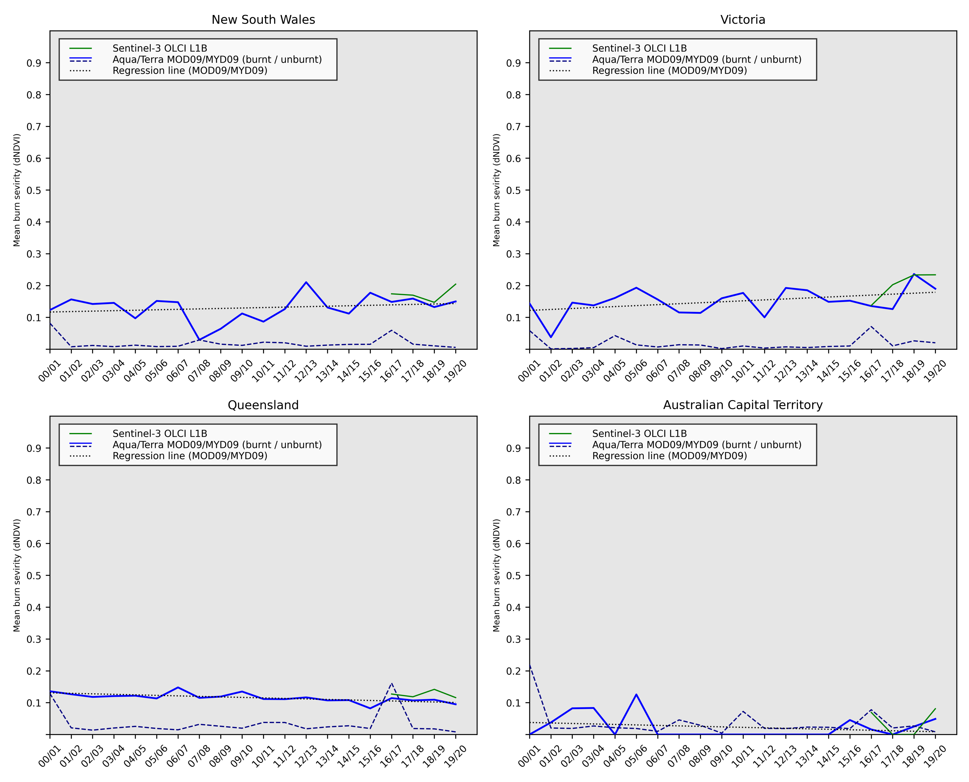
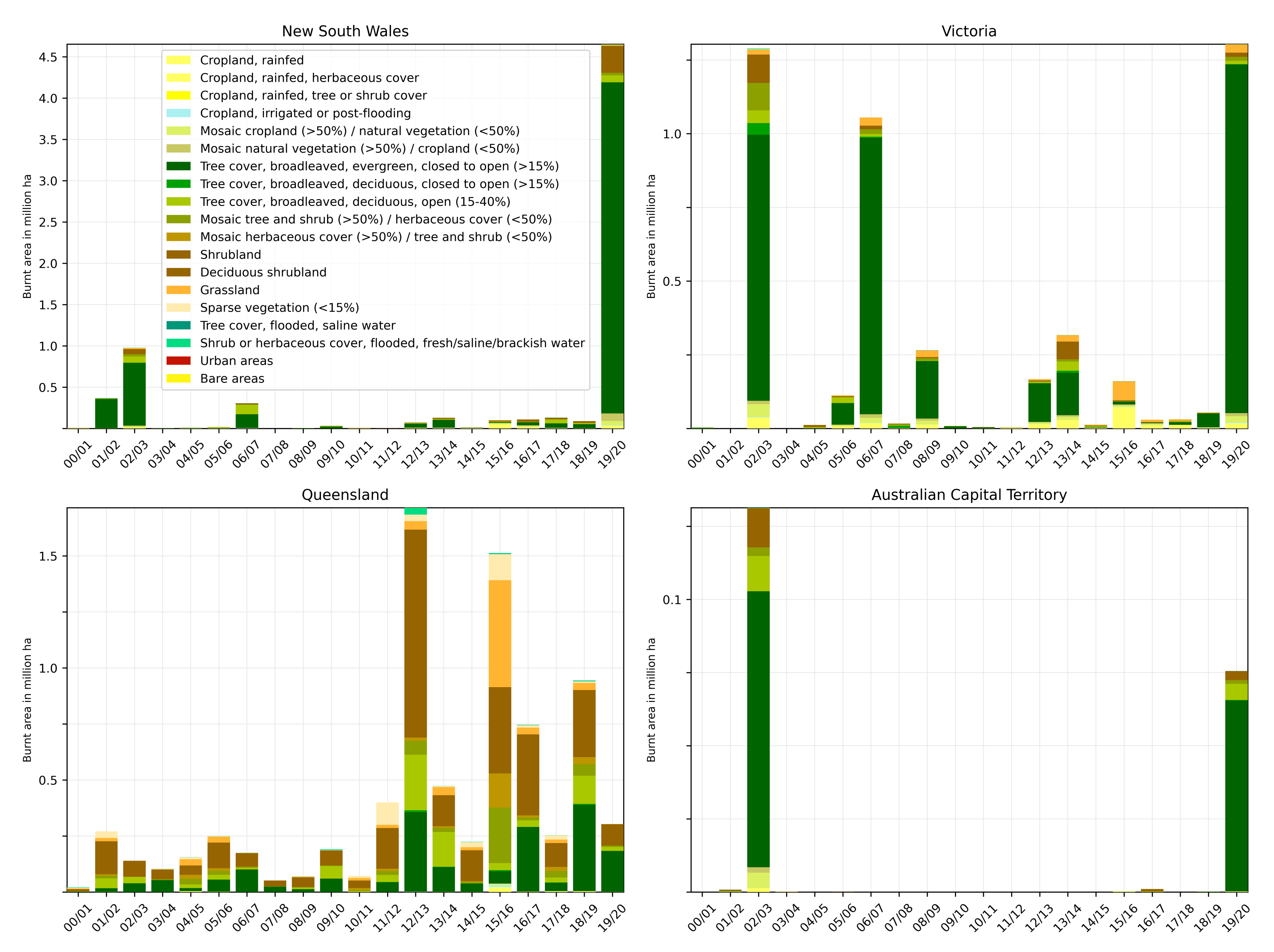
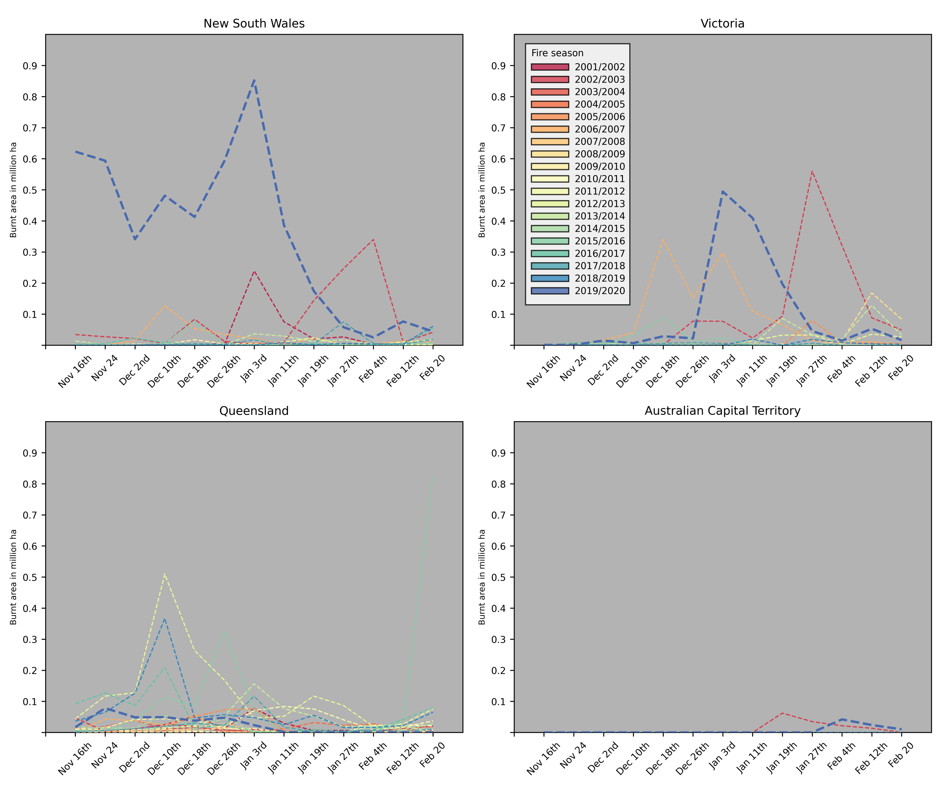
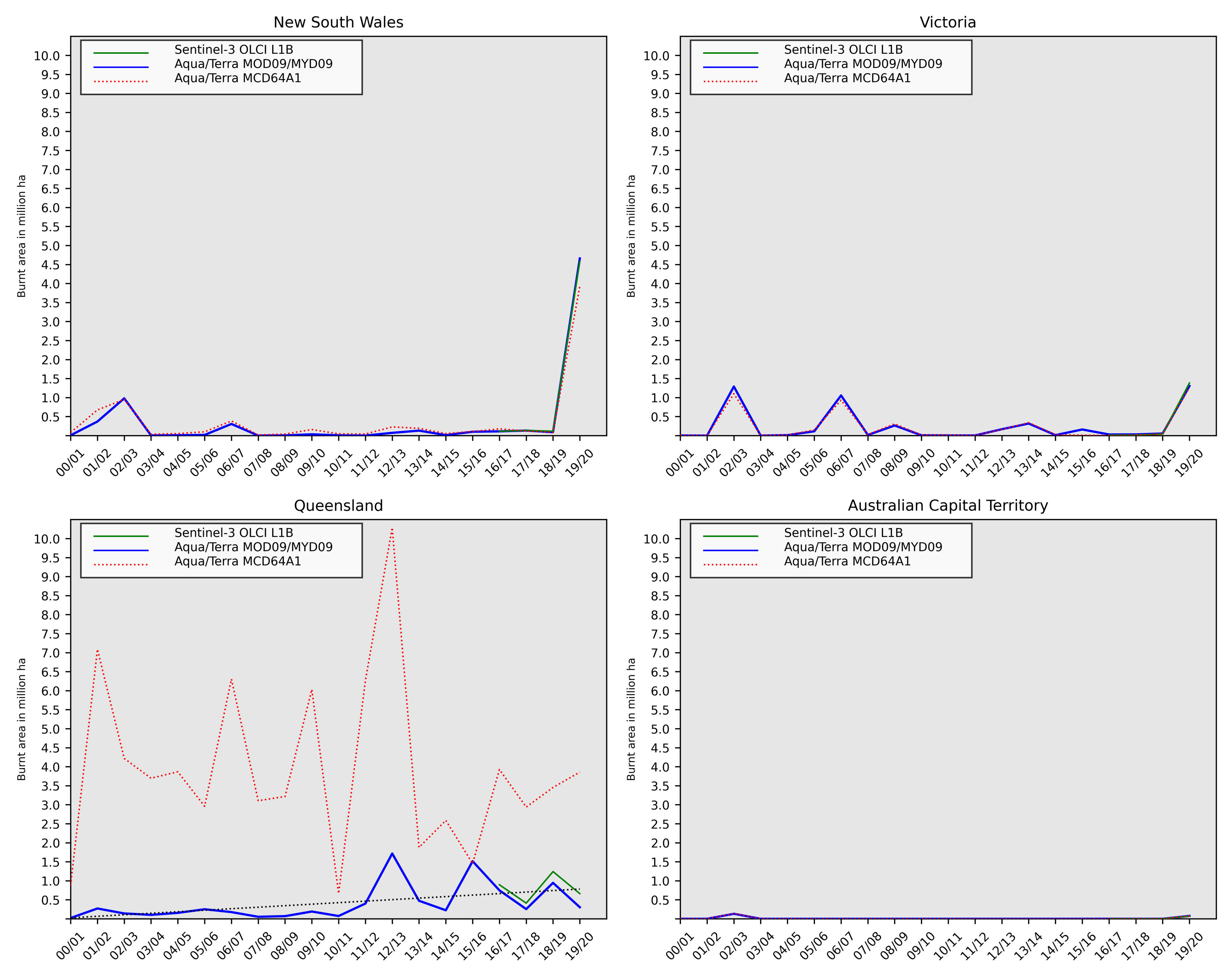
3.1. Fire Trends Regarding the States in the Study Area

Figure 4 shows the total, annual extent of burnt area for the four Australian states, and territories of interest, regarding the time period of 2000 to 2020. The results derived from Sentinel-3 OLCI data are depicted as a green line, while results regarding MODIS MOD09A1/MYD09A1 data are shown in blue. As the first one of the Sentinel-3 satellites was only launched in 2016, the analysis could only be carried out for this limited timespan. The red, dotted line represents the NASA MCD64A1 [8] burnt area dataset. The latter is included as a reference, to allow an estimation of the accuracy of the presented results. Finally, the black, dotted line is the regression line, corresponding to the MODIS MOD09/MYD09 based results.

It can be seen that the results show a high correlation of burnt area extent between the utilized DLR-GZS burnt area dataset and the MCD64A1 reference, regarding three of the four analyzed states. For Queensland, however, this is not the case. The discrepancies are due to differences in the methodologies: Unlike in the NASA dataset, burn sites where the vegetation has quickly recovered are excluded in the presented data. As stated before, wildfire is a natural phenomenon, and in many parts of Australia the regular burning of huge areas of bush and grassland vegetation is part of the natural cycle. The affected vegetation recovers quickly, some species do so even within a period of a few weeks. In the case of Queensland, these areas account for the majority of the overall burnt area. In order to confine the results to potentially harmful wildfire events, it was decided to consider burnt area in this study only when distinctive traces of burning activity could still be detected after a period of three weeks. This filtering is not performed for the generation of the MCD64A1 dataset, and as a consequence, the overall burnt area for Queensland differs considerably between the two products.

Furthermore, the figure shows that there is no linear trend in fire extent regarding New South Wales, Victoria, and the ACT. This is also reflected by

Table 3. Trend statistics regarding the extent of burnt area from 2000 to 2020. Only Queensland shows a statistically significant upward trend (highlighted in dark gray).

State	Slope	Corr. Coef.	p-Value	RMSE
New South Wales	0.054	0.31	0.18	0.962
Queensland	0.04	0.495	0.026	0.402
Victoria	0.002	0.028	0.91	0.421
ACT	0.0	−0.072	0.764	0.032

, which lists the respective statistics for Figure 4. The p-value, symbolizing the statistical significance, illustrates that there is no linear development regarding the derived trends. Complying with the common standard, a p-value below 0.05 is regarded to represent statistical significance. Such a low value is found in the case of Queensland, which features a robust, increasing trend regarding the extent of wildfires over the last two decades.

A reason for the extraordinary extent of burnt area, which is especially pronounced for the state of New South Wales, is shown in Figure A1 in the Appendix A. The burnt area extent is depicted for the past 20 years, sub-divided by month of the fire season. It can be seen that the fire activity in New South Wales reached a significant level at the beginning of November, while the main activity usually only occurs towards the end of the year. The fire activity started several weeks earlier than usual in the 2019/2020 season.

While the figures above provide a general impression by showing the fire extents over the past 20 years, this study focuses on fire severity, which is analyzed consecutively. The term is defined as a measure of the degree of environmental change caused by fire [68]. It represents a critical aspect of fire regimes, indicating the impacts on ecosystems and associated post-fire recovery [15]. The respective impact ranges from the partial consumption of litter to the complete dieback of canopy trees [69].

Figure 5 shows the yearly trend of average burn severity for the four analyzed states and territories. The green line depicts the severity results regarding Sentinel-3 OLCI, while the results for the MODIS data are depicted in blue. For the latter data source, not only the burnt areas have been investigated, but also the complete complementary area, which has not been affected by fire. This represents a cross check, showing that the developments in severity are not actually caused by unrelated factors such as climate, soil or moisture related conditions. It can be seen that the states of New South Wales and Victoria feature a general upward trend, while the development is stable or even decreasing for the ACT and Queensland.

Table 4. Trend statistics regarding the mean severity of burnt area from 2000 to 2020. Queensland features a statistically significant trend (highlighted in dark gray), while Victoria shows a trend close to statistical significance (depicted in light gray).

State	Slope	Corr. Coef.	p-Value	RMSE
New South Wales	0.001	0.208	0.378	0.038
Queensland	−0.002	−0.664	0.001	0.010
Victoria	0.003	0.423	0.06	0.037
ACT	−0.002	−0.247	0.29	0.035

shows that, even if the severity trend for New South Wales and Victoria is increasing, the p-values are too heterogeneous for these trends to be statistically significant. Only the slightly negative trend for Queensland can be considered robust. The results of the cross check are listed in

Table 5. Cross check trend statistics regarding the mean decline in vegetation fitness of area unaffected by fire, from 2000 to 2020.

State	Slope	Corr. Coef.	p-Value	RMSE
New South Wales	0.0	−0.148	0.53	0.018
Queensland	0.0	−0.044	0.85	0.038
Victoria	0.0	0.05	0.84	0.019
ACT	−0.002	−0.304	0.19	0.044

. The mentioned heterogeneity is addressed in the Discussion section.

In order to discriminate regions which account for the rising trend in New South Wales and Victoria, the study region is subdivided into regions which share similarities regarding available fuel and species composition. These are consecutively analyzed equivalent to the states. As a reasonable classification, climate zone mapping information is used. Parks et al. could show that climatic conditions, next to fuel and weather, represent a major driver of fire intensity [70]. As a next step, the climate zones featuring statistically relevant trends are further subdivided into ecological units, which are provided by the United States Geological Survey (USGS) [40]. This allows the fine-granular attribution of state-wide trends to small scale vegetation types.

The following section analyzes the climate zones contained in the study area regarding their burn severity trends. For the zones featuring developments with statistical significance, it is shown to which extent they overlap with the area of New South Wales and Victoria.

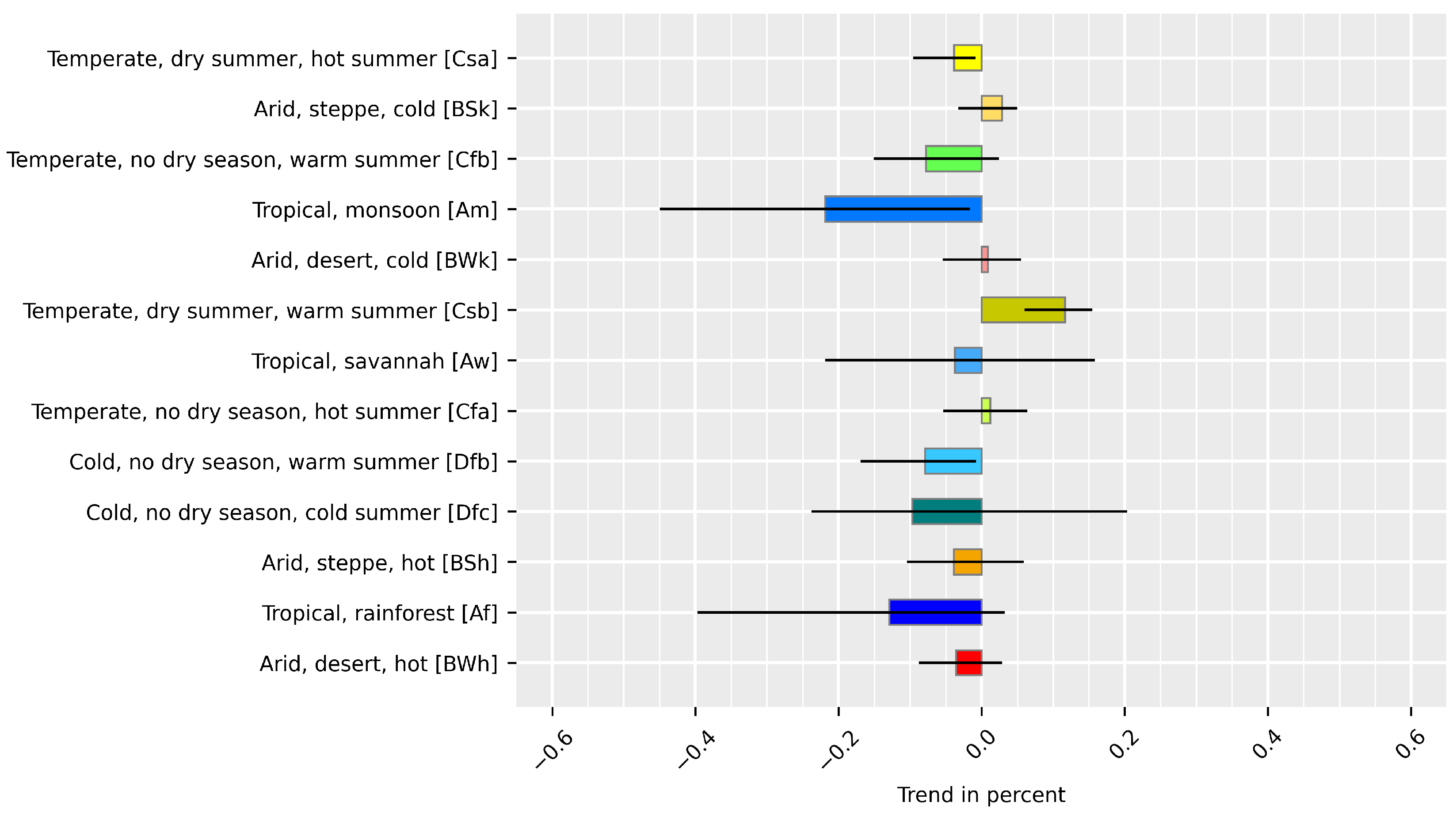
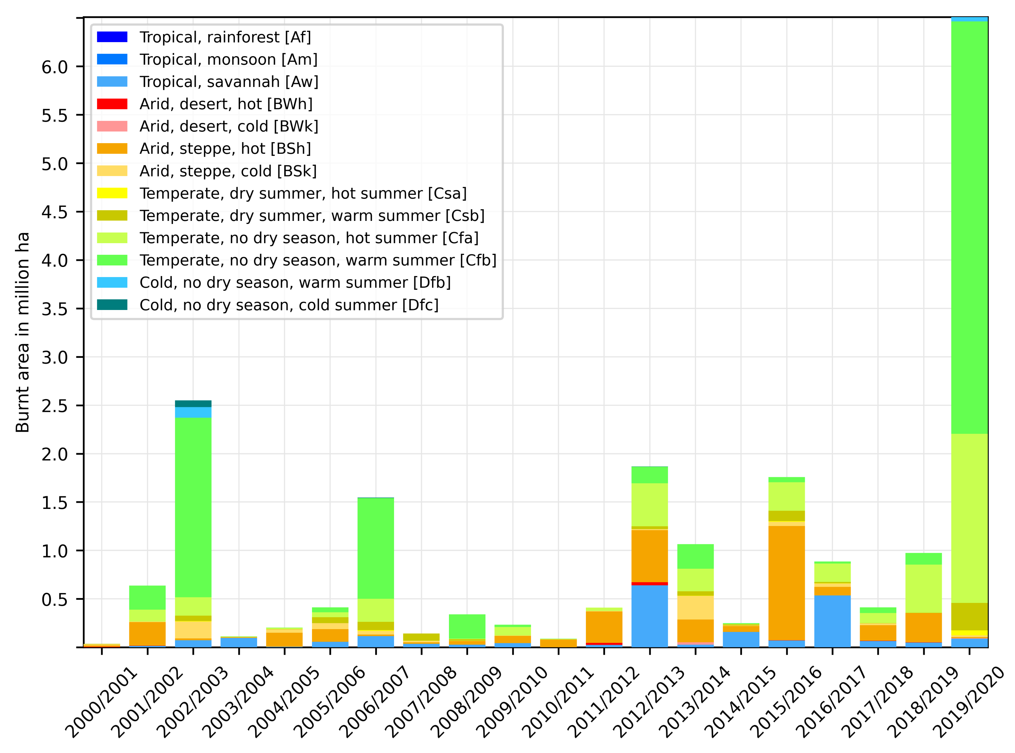
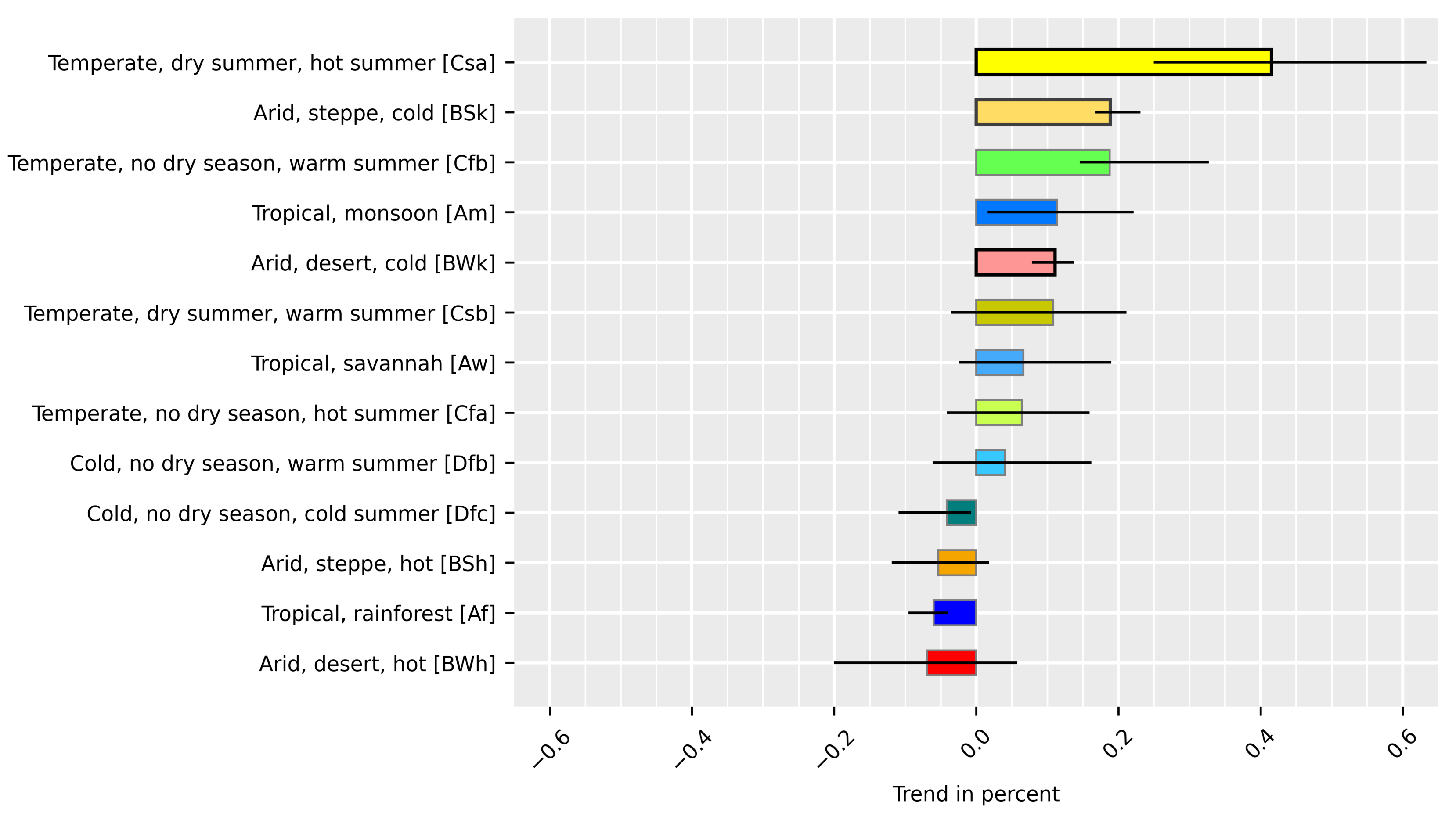
3.2. Fire Trends Regarding Climate Zones

Figure 6 shows, first and foremost, the exceptionality of the 2019/2020 wildfire events, regarding the total extent of the burnings. The calculated size reaches 6.5 million hectares, which is more than twice as high as in every other year in the analyzed time span. In addition to the total extent, a subdivision regarding the affected climate zones is shown. For this division, the Köppen–Geiger classification system published by Beck et al. (2018) [22] is used. The color scheme follows the one proposed by the authors.

Table 6. Trends regarding the size of affected area for each climate zone in the area of interest. The climate zone featuring a statistically significant trend is marked in dark gray. The one showing a trend close to statistical significance is depicted in light gray.

Class	Slope (%)	Perc 5	Perc 95	Corr. Coef.	p-Value	RMSE	Label
Csa	0.070	0.057	0.080	0.385	0.09	0.009	Temperate, dry summer, hot summer
BSk	−0.053	−0.358	0.175	−0.051	0.83	0.060	Arid, steppe, cold
Cfb	3.519	0.443	7.165	0.206	0.38	0.962	Temperate, no dry season, warm summer
Am	0.004	−0.000	0.011	0.234	0.32	0.001	Tropical, monsoon
BWk	0.020	0.000	0.045	0.223	0.34	0.005	Arid, desert, cold
Csb	0.360	0.064	0.499	0.322	0.17	0.061	Temperate, dry summer, warm summer
Aw	0.883	0.675	1.449	0.307	0.19	0.158	Tropical, savannah
Cfa	3.422	3.006	4.467	0.519	0.019	0.325	Temperate, no dry season, hot summer
Dfb	−0.061	−0.117	0.066	−0.142	0.55	0.024	Cold, no dry season, warm summer
Dfc	−0.078	−0.123	−0.047	−0.295	0.21	0.014	Cold, no dry season, cold summer
BSh	1.494	0.741	2.058	0.325	0.16	0.250	Arid, steppe, hot
Af	−0.000	−0.001	0.001	−0.022	0.93	0.000	Tropical, rainforest
BWh	0.014	−0.024	0.038	0.108	0.65	0.007	Arid, desert, hot

represents a listing of all climate zones in the area of interest together with their p-value as a measure of statistical significance. A threshold of $p\le$ 0.05 is applied to indicate the significance, the respective table row is marked in dark gray. Climate zones featuring a p-value close to statistical significance (0.05 $<p\le$ 0.1) are highlighted with light gray color.

Note that, apart from the temperate zones featuring dry winters and warm to hot summers (Cwa/Cwb), all climate zones existing in the Eastern part of Australia are affected by wildfire.

The table shows that only one climate zone satisfies the p-value condition for statistical significance (Cfa: Temperate, no dry season, hot summer). The respective correlation coefficient lies in the moderate range, even if the RMSE (Root Mean Square Error) shows a considerable oscillation around the regression line. The column “Slope (%)” shows the actual inclination of this line, given in percent. This value represents the actual trend. For this climate zone, the yearly rate is 3.4%, indicating a considerable increment in fire size over recent years.

As can be seen in Figure 7, robust trends regarding fire severity can be derived for two climate zones. First, the temperate zone featuring dry and hot summers (Csa), and second, the arid desert zone featuring cold conditions throughout the year (BWk). The first one shows an inclination of 0.42% per year on average, the second one features a value of 0.11%. The zone of arid steppe with year-round cold conditions (BSk) shows the second largest positive trend inclination, but features a p-value just above the threshold for statistical significance.

Table 7. Trends regarding fire severity for each climate zone, given in percent of increase/decrease. Climate zones featuring a statistically significant trend are marked in dark gray. The one showing a trend close to statistical significance is depicted in light gray.

Class	Slope (%)	Perc 5	Perc 95	Corr. Coef.	p-Value	RMSE	Label
Csa	0.415	0.251	0.631	0.457	0.043	0.046	Temperate, dry summer, hot summer
BSk	0.188	0.169	0.229	0.418	0.07	0.023	Arid, steppe, cold
Cfb	0.187	0.147	0.325	0.317	0.17	0.032	Temperate, no dry season, warm summer
Am	0.113	0.018	0.219	0.209	0.38	0.030	Tropical, monsoon
BWk	0.111	0.080	0.135	0.566	0.009	0.009	Arid, desert, cold
Csb	0.108	−0.033	0.209	0.123	0.61	0.050	Temperate, dry summer, warm summer
Aw	0.066	−0.022	0.188	0.126	0.6	0.030	Tropical, savannah
Cfa	0.064	−0.039	0.157	0.108	0.65	0.034	Temperate, no dry season, hot summer
Dfb	0.040	−0.059	0.160	0.07	0.77	0.033	Cold, no dry season, warm summer
Dfc	−0.040	−0.107	−0.009	−0.117	0.62	0.020	Cold, no dry season, cold summer
BSh	−0.053	−0.116	0.016	−0.17	0.47	0.017	Arid, steppe, hot
Af	−0.059	−0.093	−0.041	−0.285	0.22	0.011	Tropical, rainforest
BWh	−0.069	−0.198	0.055	−0.109	0.65	0.036	Arid, desert, hot

lists the severity trend for each climate zone.

In order to verify that the trends depicted in the above figures and tables are actually connected to fire occurrence, instead of being a general phenomenon or an effect by a cause not investigated, a cross-check has to be performed. Figure A2, which is located in the Appendix A, shows severity trends for each climate zone, where only areas are considered that have not been affected by fire. As can be expected, no general trend of increased fire severity is observable. In fact there is a generally negative development, indicating a general increase in vegetation fitness. The p-values and the correlation coefficients are generally low, meaning that there is no connection between vegetation fitness and the progression of years in these unaffected areas.

Table A1. Cross-check regarding fire severity for each climate zone.

Class	Slope (%)	Perc 5	Perc 95	Corr. Coef.	p-Value	RMSE	Label
Csa	−0.038	−0.093	−0.010	−0.141	0.55	0.015	Temperate, dry summer, hot summer
BSk	0.028	−0.030	0.047	0.158	0.51	0.010	Arid, steppe, cold
Cfb	−0.077	−0.148	0.022	−0.135	0.57	0.032	Temperate, no dry season, warm summer
Am	−0.218	−0.447	−0.018	−0.142	0.55	0.087	Tropical, monsoon
BWk	0.008	−0.052	0.053	0.048	0.84	0.010	Arid, desert, cold
Csb	0.116	0.061	0.152	0.292	0.21	0.022	Temperate, dry summer, warm summer
Aw	−0.037	−0.216	0.156	−0.029	0.9	0.072	Tropical, savannah
Cfa	0.012	−0.051	0.061	0.028	0.91	0.025	Temperate, no dry season, hot summer
Dfb	−0.079	−0.167	−0.009	−0.109	0.65	0.041	Cold, no dry season, warm summer
Dfc	−0.096	−0.235	0.201	−0.111	0.64	0.050	Cold, no dry season, cold summer
BSh	−0.038	−0.102	0.057	−0.072	0.76	0.030	Arid, steppe, hot
Af	−0.129	−0.395	0.030	−0.079	0.74	0.094	Tropical, rainforest
BWh	−0.035	−0.085	0.027	−0.125	0.6	0.016	Arid, desert, hot

, which can be found in the Appendix A, shows the statistical information regarding the cross-check.

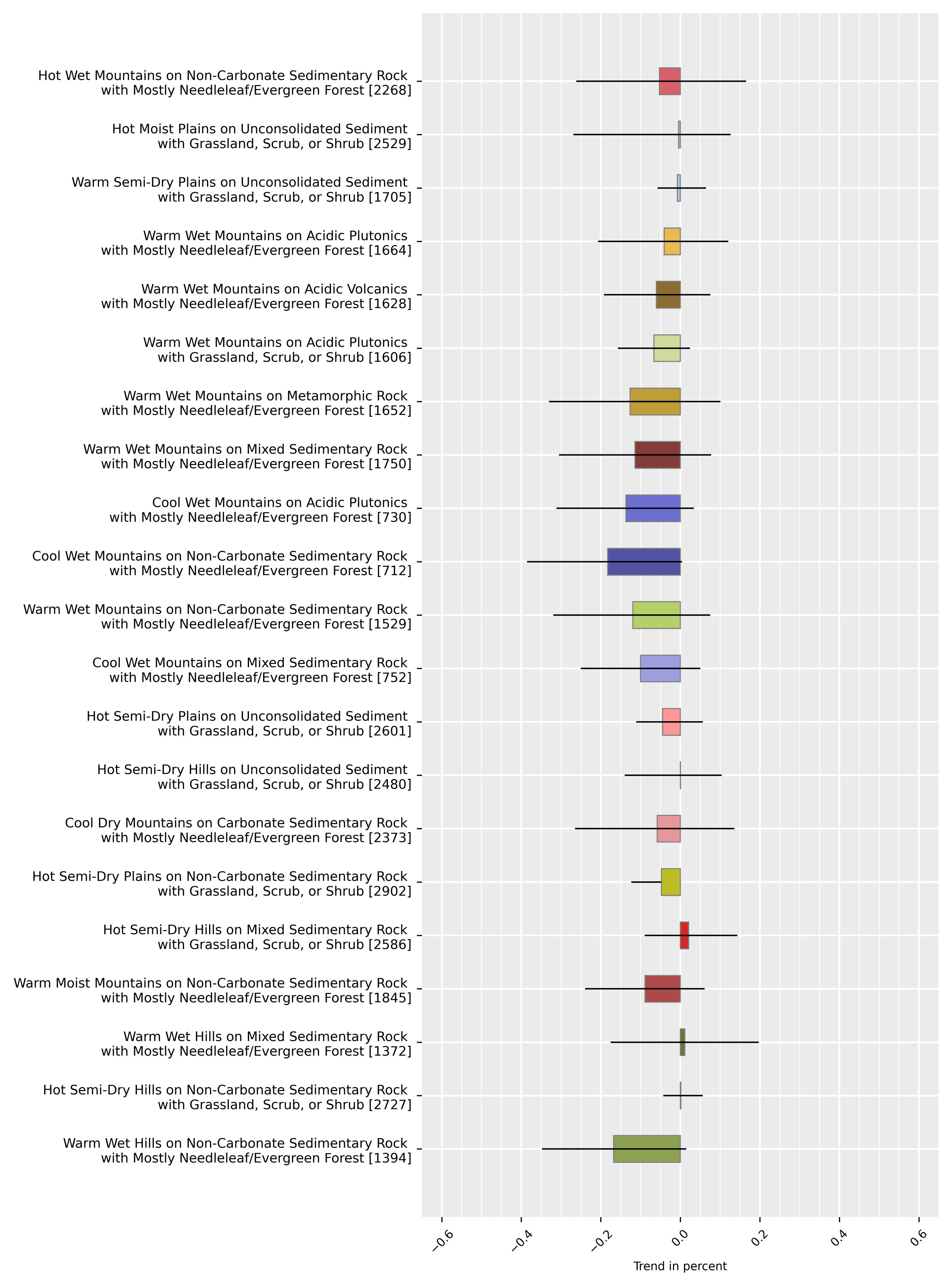
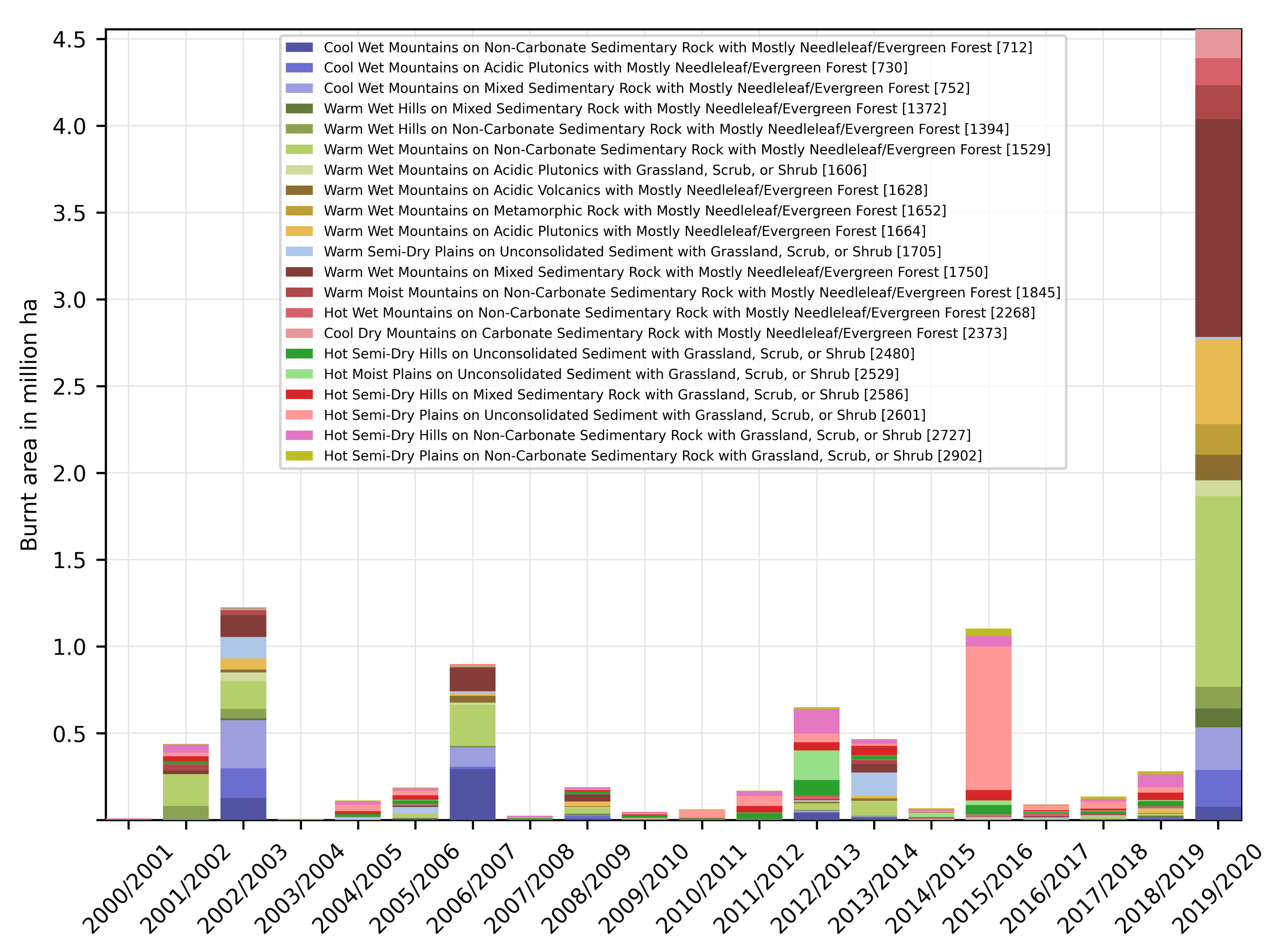
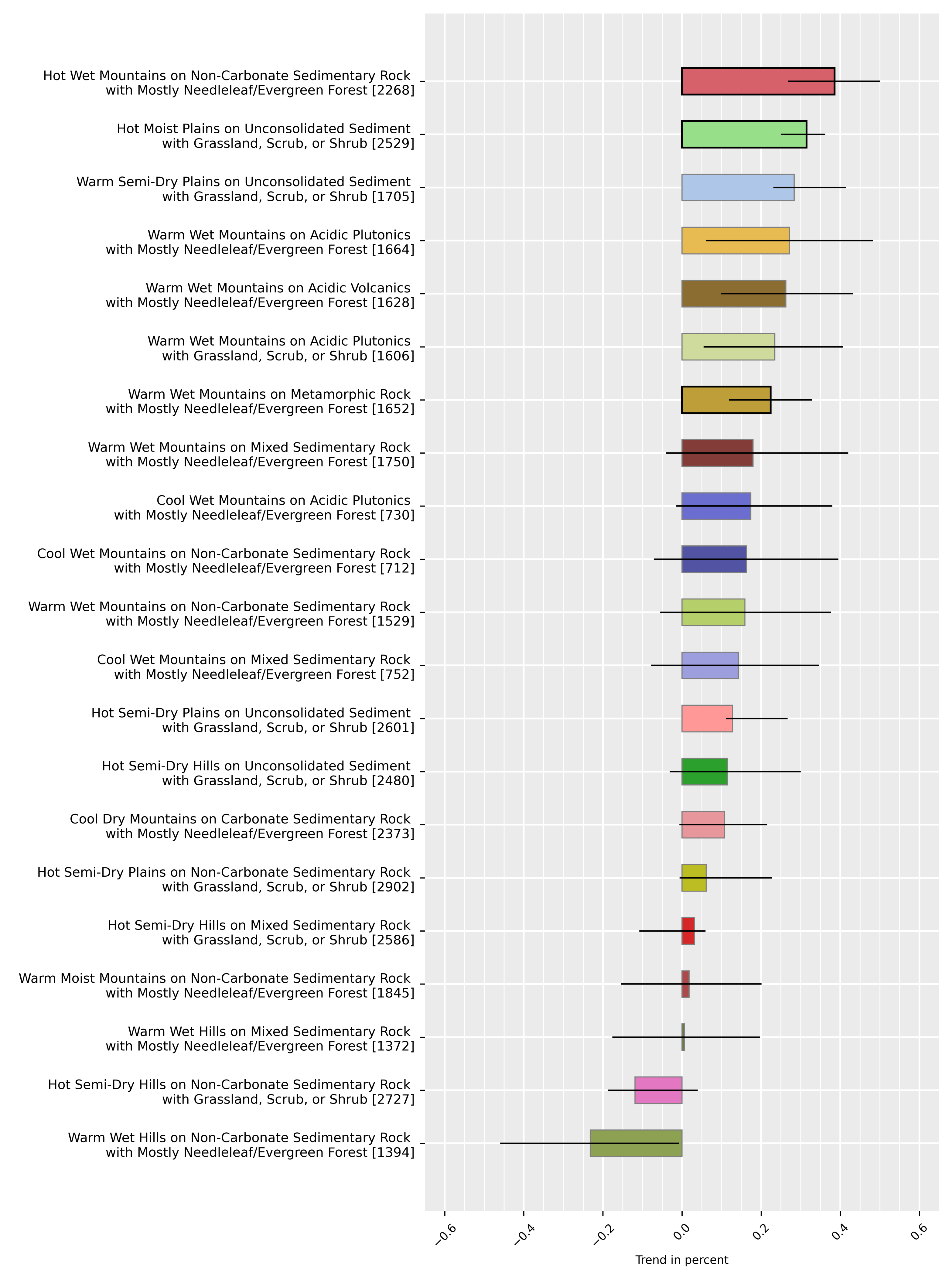
3.3. Fire Trends Regarding Ecological Units

In order to draw conclusions regarding the vegetation types causing the increasing severity trends in some of the climate zones, the analysis is also carried out on the basis of ecological units. These units feature a higher spatial and thematic resolution, and are thus better suited for analyses on a smaller scale.

For the incorporation of ecological units, the Global Ecological Land Units global dataset provided by the United States Geological Survey (USGS) [40] is used. The ecological units are a combination of bioclimate region, landform type, surficial lithology, and land cover information [71], and allow for a very high thematic resolution. This results in more than 3600 different units covering the area of interest. In order to reduce the number of units to be analyzed to an appropriate level, a subset is generated from the original data in a preceding step. This subset contains all ecological units which were affected by the 2019/2020 burnings and covered more than 1% of the burnt area. Furthermore, it comprises all ecological units covering more than 1% of the area of interest.

Figure 8 shows the analysis results of the total burnt area extent development, regarding the ecological units. It can be seen that the three most prominent units (1750, 1529, and 1664) feature either needleleaf or evergreen forest, which has not been the case in former years. Statistically significant results can, however, only be derived for the class of “Hot Wet Mountains on Non-Carbonate Sedimentary Rock with Mostly Needleleaf/Evergreen Forest” (2268). The statistical results are found in

Table A2. Trends regarding the burnt area size for each ecological unit in the area of interest. The ecological unit featuring a statistically significant trend is marked in dark gray. Ecological units showing trends close to statistical significance are depicted in light gray.

Class	Slope (%)	Perc 5	Perc 95	Corr. Coef.	p-Value	RMSE	Label
2268	0.263	0.150	0.373	0.456	0.04	0.029	Hot Wet Mountains on Non-Carbonate Sedimentary Rock with Mostly Needleleaf/Evergreen Forest
1712	0.058	0.028	0.089	0.418	0.07	0.007	Warm Semi-Dry Plains on Unconsolidated Sediment with Mostly Cropland
2529	0.108	0.029	0.229	0.17	0.47	0.036	Hot Moist Plains on Unconsolidated Sediment with Grassland, Scrub, or Shrub
1705	−0.064	−0.132	0.050	−0.1	0.68	0.037	Warm Semi-Dry Plains on Unconsolidated Sediment with Grassland, Scrub, or Shrub
1664	0.652	0.265	0.998	0.357	0.12	0.098	Warm Wet Mountains on Acidic Plutonics with Mostly Needleleaf/Evergreen Forest
1628	0.184	0.063	0.294	0.329	0.15	0.030	Warm Wet Mountains on Acidic Volcanics with Mostly Needleleaf/Evergreen Forest
1606	0.072	−0.015	0.160	0.189	0.42	0.021	Warm Wet Mountains on Acidic Plutonics with Grassland, Scrub, or Shrub
1734	0.095	0.038	0.150	0.371	0.10	0.013	Warm Wet Mountains on Non-Acidic Volcanics with Mostly Needleleaf/Evergreen Forest
1652	0.253	0.116	0.394	0.38	0.09	0.035	Warm Wet Mountains on Metamorphic Rock with Mostly Needleleaf/Evergreen Forest
1750	1.581	0.567	2.503	0.336	0.14	0.255	Warm Wet Mountains on Mixed Sedimentary Rock with Mostly Needleleaf/Evergreen Forest
730	0.108	−0.103	0.321	0.109	0.64	0.056	Cool Wet Mountains on Acidic Plutonics with Mostly Needleleaf/Evergreen Forest
712	−0.161	−0.417	0.095	−0.136	0.56	0.068	Cool Wet Mountains on Non-Carbonate Sedimentary Rock with Mostly Needleleaf/Evergreen Forest
1529	1.097	0.275	1.968	0.264	0.26	0.231	Warm Wet Mountains on Non-Carbonate Sedimentary Rock with Mostly Needleleaf/Evergreen Forest
752	−0.023	−0.311	0.274	−0.017	0.94	0.079	Cool Wet Mountains on Mixed Sedimentary Rock with Mostly Needleleaf/Evergreen Forest
2601	0.759	0.132	1.083	0.248	0.29	0.171	Hot Semi-Dry Plains on Unconsolidated Sediment with Grassland, Scrub, or Shrub
2480	0.105	0.058	0.153	0.279	0.23	0.020	Hot Semi-Dry Hills on Unconsolidated Sediment with Grassland, Scrub, or Shrub
2373	0.231	0.111	0.355	0.38	0.09	0.032	Cool Dry Mountains on Carbonate Sedimentary Rock with Mostly Needleleaf/Evergreen Forest
2902	0.068	0.015	0.083	0.405	0.08	0.008	Hot Semi-Dry Plains on Non-Carbonate Sedimentary Rock with Grassland, Scrub, or Shrub
2621	0.050	0.030	0.093	0.273	0.24	0.010	Hot Semi-Dry Plains on Unconsolidated Sediment with Sparse Vegetation
2711	4.196	−0.001	0.002	0.259	0.27	0.000	Hot Dry Plains on Unconsolidated Sediment with Bare area
2586	0.106	0.043	0.165	0.313	0.18	0.018	Hot Semi-Dry Hills on Mixed Sedimentary Rock with Grassland, Scrub, or Shrub
2606	0.003	−0.006	0.018	0.072	0.76	0.002	Hot Semi-Dry Plains on Mixed Sedimentary Rock with Sparse Vegetation
1845	0.222	0.074	0.359	0.3	0.19	0.040	Warm Moist Mountains on Non-Carbonate Sedimentary Rock with Mostly Needleleaf/Evergreen Forest
2614	0.019	0.012	0.031	0.337	0.15	0.003	Hot Semi-Dry Plains on Mixed Sedimentary Rock with Grassland, Scrub, or Shrub
1372	0.151	0.066	0.232	0.378	0.10	0.021	Warm Wet Hills on Mixed Sedimentary Rock with Mostly Needleleaf/Evergreen Forest
2822	4.034	−0.003	0.001	0.061	0.8	0.000	Hot Dry Plains on Unconsolidated Sediment with Sparse Vegetation
2784	−0.000	−0.007	0.004	−0.06	0.8	0.000	Hot Semi-Dry Plains on Non-Carbonate Sedimentary Rock with Sparse Vegetation
1849	−0.019	−0.028	−0.007	−0.307	0.19	0.003	Warm Semi-Dry Plains on Unconsolidated Sediment with Sparse Vegetation
2727	0.146	0.092	0.277	0.255	0.28	0.032	Hot Semi-Dry Hills on Non-Carbonate Sedimentary Rock with Grassland, Scrub, or Shrub
2791	0.008	0.007	0.033	0.085	0.72	0.005	Hot Dry Plains on Unconsolidated Sediment with Swampy or Often Flooded Vegetation
1394	0.024	−0.103	0.140	0.045	0.84	0.031	Warm Wet Hills on Non-Carbonate Sedimentary Rock with Mostly Needleleaf/Evergreen Forest

in the Appendix A.

Figure 9 shows the severity trends regarding ecological units, equivalent to the climate zone analysis above. Similar to the burnt area extent analysis, stable trends can be derived for two classes featuring either needleleaf or evergreen forest. These classes are “Hot Wet Mountains on Non-Carbonate Sedimentary Rock with Mostly Needleleaf/Evergreen Forest (2268)” and “Warm Wet Mountains on Metamorphic Rock with Mostly Needleleaf/Evergreen Forest (1652)”. Two further units feature p-values close to statistical significance, and are thus worth being considered: “Warm Semi-Dry Plains on Unconsolidated Sediment with Mostly Cropland (1712)” and “Hot Moist Plains on Unconsolidated Sediment with Grassland, Scrub, or Shrub (2529)”. All respective statistical information is found in

Table A3. Trends regarding the fire severity for each ecological unit in the area of interest. Ecological units featuring statistically significant trends are marked in dark gray. The ones showing trends close to statistical significance are depicted in light gray.

Class	Slope (%)	Perc 5	Perc 95	Corr. Coef.	p-Value	RMSE	Label
2268	0.385	0.269	0.499	0.589	0.006	0.030	Hot Wet Mountains on Non-Carbonate Sedimentary Rock with Mostly Needleleaf/Evergreen Forest
1712	0.326	0.177	0.453	0.385	0.09	0.045	Warm Semi-Dry Plains on Unconsolidated Sediment with Mostly Cropland
2529	0.314	0.251	0.360	0.519	0.019	0.029	Hot Moist Plains on Unconsolidated Sediment with Grassland, Scrub, or Shrub
1705	0.283	0.232	0.413	0.341	0.14	0.044	Warm Semi-Dry Plains on Unconsolidated Sediment with Grassland, Scrub, or Shrub
1664	0.271	0.063	0.480	0.277	0.236	0.054	Warm Wet Mountains on Acidic Plutonics with Mostly Needleleaf/Evergreen Forest
1628	0.262	0.100	0.429	0.318	0.171	0.045	Warm Wet Mountains on Acidic Volcanics with Mostly Needleleaf/Evergreen Forest
1606	0.234	0.056	0.404	0.269	0.251	0.048	Warm Wet Mountains on Acidic Plutonics with Grassland, Scrub, or Shrub
1734	0.224	0.052	0.407	0.259	0.269	0.048	Warm Wet Mountains on Non-Acidic Volcanics with Mostly Needleleaf/Evergreen Forest
1652	0.224	0.120	0.326	0.45	0.046	0.025	Warm Wet Mountains on Metamorphic Rock with Mostly Needleleaf/Evergreen Forest
1750	0.179	−0.038	0.418	0.161	0.498	0.063	Warm Wet Mountains on Mixed Sedimentary Rock with Mostly Needleleaf/Evergreen Forest
730	0.173	−0.012	0.378	0.179	0.450	0.055	Cool Wet Mountains on Acidic Plutonics with Mostly Needleleaf/Evergreen Forest
712	0.163	−0.069	0.393	0.148	0.533	0.062	Cool Wet Mountains on Non-Carbonate Sedimentary Rock with Mostly Needleleaf/Evergreen Forest
1529	0.158	−0.053	0.374	0.158	0.504	0.057	Warm Wet Mountains on Non-Carbonate Sedimentary Rock with Mostly Needleleaf/Evergreen Forest
752	0.142	−0.076	0.344	0.145	0.543	0.056	Cool Wet Mountains on Mixed Sedimentary Rock with Mostly Needleleaf/Evergreen Forest
2601	0.127	0.113	0.265	0.212	0.37	0.034	Hot Semi-Dry Plains on Unconsolidated Sediment with Grassland, Scrub, or Shrub
2480	0.114	−0.029	0.298	0.176	0.46	0.037	Hot Semi-Dry Hills on Unconsolidated Sediment with Grassland, Scrub, or Shrub
2373	0.107	−0.004	0.213	0.217	0.357	0.027	Cool Dry Mountains on Carbonate Sedimentary Rock with Mostly Needleleaf/Evergreen Forest
2902	0.061	−0.004	0.225	0.089	0.71	0.039	Hot Semi-Dry Plains on Non-Carbonate Sedimentary Rock with Grassland, Scrub, or Shrub
2621	0.056	−0.060	0.138	0.113	0.64	0.028	Hot Semi-Dry Plains on Unconsolidated Sediment with Sparse Vegetation
2711	0.035	0.005	0.062	0.259	0.27	0.007	Hot Dry Plains on Unconsolidated Sediment with Bare area
2586	0.031	−0.106	0.057	0.05	0.83	0.036	Hot Semi-Dry Hills on Mixed Sedimentary Rock with Grassland, Scrub, or Shrub
2606	0.022	−0.022	0.128	0.054	0.82	0.024	Hot Semi-Dry Plains on Mixed Sedimentary Rock with Sparse Vegetation
1845	0.017	−0.152	0.199	0.023	0.924	0.045	Warm Moist Mountains on Non-Carbonate Sedimentary Rock with Mostly Needleleaf/Evergreen Forest
2614	0.010	−0.121	0.066	0.019	0.94	0.033	Hot Semi-Dry Plains on Mixed Sedimentary Rock with Grassland, Scrub, or Shrub
1372	0.005	−0.174	0.194	0.007	0.977	0.046	Warm Wet Hills on Mixed Sedimentary Rock with Mostly Needleleaf/Evergreen Forest
2822	−0.018	−0.019	0.006	−0.094	0.69	0.011	Hot Dry Plains on Unconsolidated Sediment with Sparse Vegetation
2784	−0.028	−0.122	0.074	−0.066	0.78	0.025	Hot Semi-Dry Plains on Non-Carbonate Sedimentary Rock with Sparse Vegetation
1849	−0.078	−0.140	0.047	−0.15	0.53	0.029	Warm Semi-Dry Plains on Unconsolidated Sediment with Sparse Vegetation
2727	−0.118	−0.185	0.037	−0.211	0.37	0.031	Hot Semi-Dry Hills on Non-Carbonate Sedimentary Rock with Grassland, Scrub, or Shrub
2791	−0.123	−0.298	−0.087	−0.22	0.35	0.031	Hot Dry Plains on Unconsolidated Sediment with Swampy or Often Flooded Vegetation
1394	−0.231	−0.457	−0.009	−0.218	0.355	0.059	Warm Wet Hills on Non-Carbonate Sedimentary Rock with Mostly Needleleaf/Evergreen Forest

in the Appendix A.

The increasing burn severity for some classes can be linked to a higher degree of combustion. Other reasons include the higher amount of combustible biomass, the concern of younger, healthier vegetation, or the exposure of different vegetation types.

The cross-check, conducted for areas which have not been affected by fire, shows the expected, generally negative trend. The derived fire severity trends presented above are therefore demonstrably caused by wildfire activity. Figure A3 shows the trend for each ecological unit. All respective statistical information is found in

Table A4. Cross-check regarding fire severity for each ecological unit in the area of interest.

Class	Slope (%)	Perc 5	Perc 95	Corr. Coef.	p-Value	RMSE	Label
2268	−0.052	−0.259	0.163	−0.053	0.824	0.057	Hot Wet Mountains on Non-Carbonate Sedimentary Rock with Mostly Needleleaf/Evergreen Forest
1712	0.012	−0.006	0.039	0.081	0.73	0.008	Warm Semi-Dry Plains on Unconsolidated Sediment with Mostly Cropland
2529	−0.004	−0.267	0.124	−0.003	0.99	0.070	Hot Moist Plains on Unconsolidated Sediment with Grassland, Scrub, or Shrub
1705	−0.007	−0.055	0.062	−0.034	0.89	0.012	Warm Semi-Dry Plains on Unconsolidated Sediment with Grassland, Scrub, or Shrub
1664	−0.040	−0.204	0.118	−0.055	0.818	0.042	Warm Wet Mountains on Acidic Plutonics with Mostly Needleleaf/Evergreen Forest
1628	−0.060	−0.190	0.073	−0.099	0.679	0.034	Warm Wet Mountains on Acidic Volcanics with Mostly Needleleaf/Evergreen Forest
1606	−0.066	−0.154	0.022	−0.166	0.484	0.022	Warm Wet Mountains on Acidic Plutonics with Grassland, Scrub, or Shrub
1734	−0.110	−0.257	0.030	−0.159	0.501	0.039	Warm Wet Mountains on Non-Acidic Volcanics with Mostly Needleleaf/Evergreen Forest
1652	−0.126	−0.328	0.099	−0.125	0.600	0.057	Warm Wet Mountains on Metamorphic Rock with Mostly Needleleaf/Evergreen Forest
1750	−0.113	−0.303	0.075	−0.13	0.586	0.050	Warm Wet Mountains on Mixed Sedimentary Rock with Mostly Needleleaf/Evergreen Forest
730	−0.136	−0.309	0.032	−0.171	0.469	0.045	Cool Wet Mountains on Acidic Plutonics with Mostly Needleleaf/Evergreen Forest
712	−0.182	−0.383	0.002	−0.2	0.397	0.051	Cool Wet Mountains on Non-Carbonate Sedimentary Rock with Mostly Needleleaf/Evergreen Forest
1529	−0.119	−0.317	0.073	−0.134	0.573	0.050	Warm Wet Mountains on Non-Carbonate Sedimentary Rock with Mostly Needleleaf/Evergreen Forest
752	−0.100	−0.248	0.048	−0.148	0.533	0.038	Cool Wet Mountains on Mixed Sedimentary Rock with Mostly Needleleaf/Evergreen Forest
2601	−0.044	−0.109	0.055	−0.089	0.71	0.028	Hot Semi-Dry Plains on Unconsolidated Sediment with Grassland, Scrub, or Shrub
2480	0.000	−0.137	0.102	0.001	1.0	0.033	Hot Semi-Dry Hills on Unconsolidated Sediment with Grassland, Scrub, or Shrub
2373	−0.058	−0.262	0.134	−0.061	0.799	0.055	Cool Dry Mountains on Carbonate Sedimentary Rock with Mostly Needleleaf/Evergreen Forest
2902	−0.047	−0.121	−0.049	−0.112	0.64	0.024	Hot Semi-Dry Plains on Non-Carbonate Sedimentary Rock with Grassland, Scrub, or Shrub
2621	−0.054	−0.193	0.092	−0.093	0.7	0.033	Hot Semi-Dry Plains on Unconsolidated Sediment with Sparse Vegetation
2711	−0.013	−0.051	0.036	−0.062	0.8	0.012	Hot Dry Plains on Unconsolidated Sediment with Bare area
2586	0.021	−0.087	0.141	0.042	0.86	0.029	Hot Semi-Dry Hills on Mixed Sedimentary Rock with Grassland, Scrub, or Shrub
2606	−0.090	−0.250	0.047	−0.109	0.65	0.047	Hot Semi-Dry Plains on Mixed Sedimentary Rock with Sparse Vegetation
1845	−0.088	−0.237	0.059	−0.123	0.605	0.041	Warm Moist Mountains on Non-Carbonate Sedimentary Rock with Mostly Needleleaf/Evergreen Forest
2614	−0.050	−0.147	0.094	−0.086	0.72	0.033	Hot Semi-Dry Plains on Mixed Sedimentary Rock with Grassland, Scrub, or Shrub
1372	0.011	−0.173	0.195	0.014	0.954	0.048	Warm Wet Hills on Mixed Sedimentary Rock with Mostly Needleleaf/Evergreen Forest
2822	−0.025	−0.071	0.037	−0.096	0.69	0.015	Hot Dry Plains on Unconsolidated Sediment with Sparse Vegetation
2784	−0.096	−0.196	0.024	−0.167	0.48	0.032	Hot Semi-Dry Plains on Non-Carbonate Sedimentary Rock with Sparse Vegetation
1849	−0.012	−0.035	0.008	−0.093	0.7	0.007	Warm Semi-Dry Plains on Unconsolidated Sediment with Sparse Vegetation
2727	0.001	−0.040	0.054	0.002	0.99	0.031	Hot Semi-Dry Hills on Non-Carbonate Sedimentary Rock with Grassland, Scrub, or Shrub
2791	−0.261	−0.350	−0.164	−0.319	0.17	0.044	Hot Dry Plains on Unconsolidated Sediment with Swampy or Often Flooded Vegetation
1394	−0.167	−0.346	0.013	−0.194	0.413	0.049	Warm Wet Hills on Non-Carbonate Sedimentary Rock with Mostly Needleleaf/Evergreen Forest

in the Appendix A.

Figure 10 shows a section of the two ecological units with a statistically significant increase in fire severity during the analyzed time span. The figure represents a detailed view of the North-Eastern part of New South Wales, where these two ecological units overlap with the area affected by the 2019/2020 wildfires.

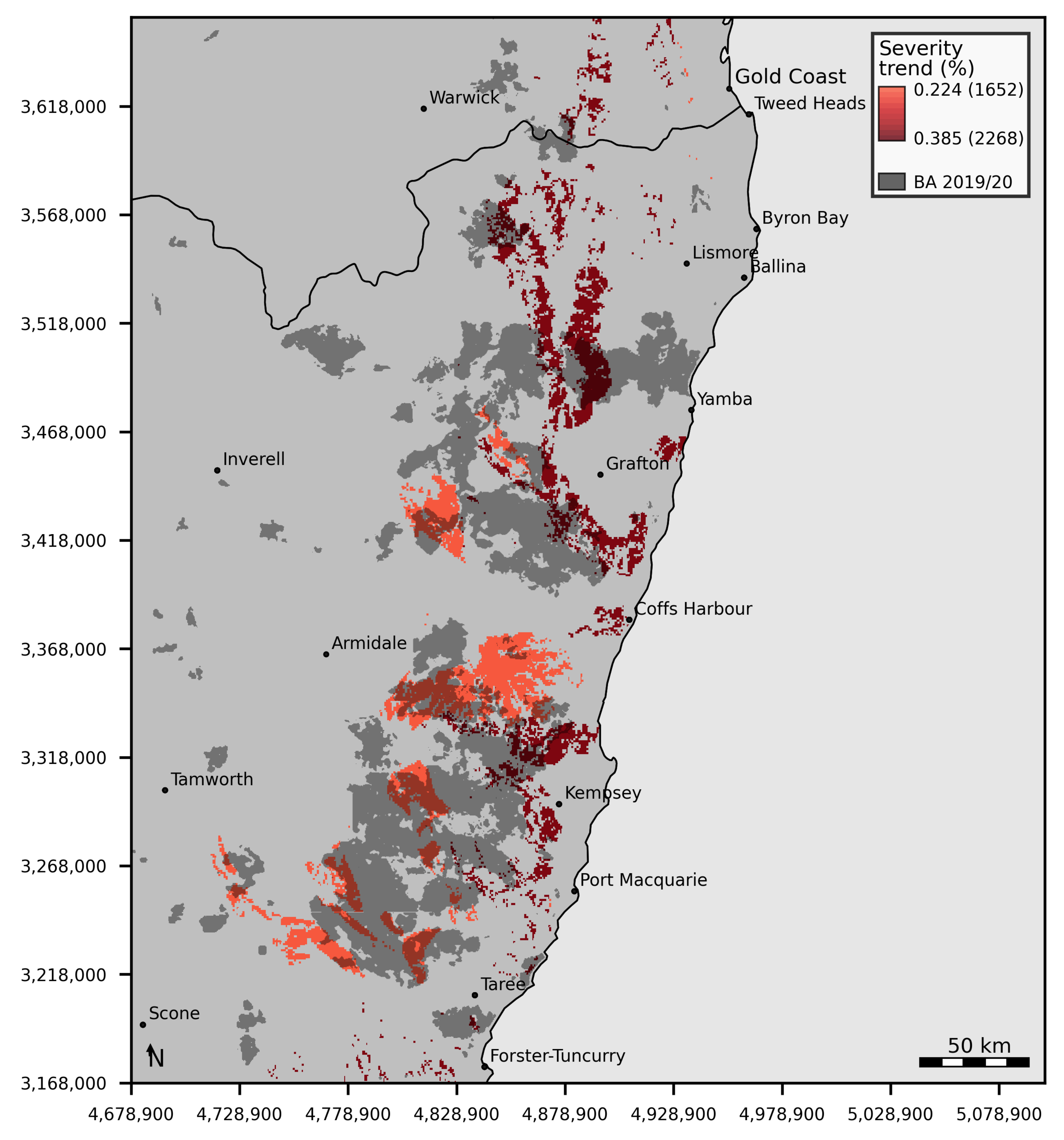
3.4. Combination of Results from Different Levels

Table 8. Percentage of area covered by relevant climate zones, regarding New South Wales and Victoria.

Climate Zone	Area Portion (%)		Label
	NSW	VIC
BWk	3.8	3.3	Arid, desert, cold
BSk	17.9	36.7	Arid, steppe, cold
Csa	0.16	1.6	Temperate, dry summer, hot summer
Cfa	19.1	1.9	Temperate, no dry season, hot summer

lists how much area of New South Wales and Victoria is covered by the relevant climate zones. Features are considered relevant if they show a trend matching or being close to statistical significance regarding burn extent or severity. Two of these zones—BSk and Cfa—cover significant portions of the two states.

Table 9. Percentage of area covered by relevant ecological units, regarding New South Wales and Victoria.

Ecological Zone	Area Portion (%)				Label
	NSW		VIC
	BSk	Cfa	BSk	Cfa
1372	-	0.1	-	-	Warm Wet Hills on Mixed Sedimentary Rock with Mostly Needleleaf/Evergreen Forest
1652	-	0.9	-	-	Warm Wet Mountains on Metamorphic Rock with Mostly Needleleaf/Evergreen Forest
1712	36.3	1.4	52.3	3.7	Warm Semi-Dry Plains on Unconsolidated Sediment with Mostly Cropland
2268	-	2.9	-	-	Hot Wet Mountains on Non-Carbonate Sedimentary Rock with Mostly Needleleaf/Evergreen Forest
2373	-	2.4	-	-	Cool Dry Mountains on Carbonate Sedimentary Rock with Mostly Needleleaf/Evergreen Forest
2529	-	-	-	-	Hot Moist Plains on Unconsolidated Sediment with Grassland, Scrub, or Shrub
2902	-	-	-	-	Hot Semi-Dry Plains on Non-Carbonate Sedimentary Rock with Grassland, Scrub, or Shrub

lists, equivalent to Table 8, how much of the area of the relevant climate zones is covered by relevant ecological units. It can be seen that unit 1712 covers 36.3% of the area of the BSk climate zone in New South Wales, and even 52.3% of this zone in Victoria. However, this unit contains mostly cropland, and thus the fire activity has to be attributed in large part to agricultural burnings. While it is interesting to note that the burn severity rises on agricultural areas, this study targets the activity of potentially harmful wildfires, and is thus not concerned with controlled, anthropogenic fires. Ecological unit 1712, and with it the BSk climate zone, is therefore considered largely irrelevant for this study. The remaining zone is Cfa, which features a temperate climate with hot summers, and without a dry season. Unit 2268, “Hot Wet Mountains on Non-Carbonate Sedimentary Rock with Mostly Needleleaf/Evergreen Forest”, shows the highest trends of all analyzed ecological units, both regarding fire extent and fire severity. The unit features an increasing trend of 0.26% on annual average regarding extent, and 0.39% regarding burn severity. Both trends are shown to be robust, indicated by their statistical significance. A similar trend can also be seen for unit 1652, “Warm Wet Mountains on Metamorphic Rock with Mostly Needleleaf/Evergreen Forest”, which shows an increasing burn severity of 0.2% on annual average.

Apart from the agricultural area, all units located within this climate zone featuring increasing severity trends contain needleleaf or evergreen forest.

This development is also discernible in Figure 11, which shows the affected vegetation types and the respective size in hectares for each of the four exposed states and territories, regarding the period of 2000 to 2020. Yearly land cover information of the ESA CCI-LC (Climate Change Initiative—Land Cover) dataset ([39]) has been used in order to derive the present vegetation types for each respective year. For New South Wales and Victoria, it can be seen that forests represent the predominantly affected vegetation type of the burnings in 2019/2020. The presented figures and statistics indicate that ecologically valuable, woody vegetation is increasingly affected in the study area.

4. Discussion

While the inter-annual variability in fire activity complicates and in some cases prohibits the derivation of statistically significant trends, several expressive conclusions could be drawn for some of the investigated climate zones and ecological units.

Steady increases regarding burn severity could be found for the climate zones BSk and Cfa, which cover significant parts of New South Wales and Victoria. These development could be traced back to several ecological units, residing inside these climate zones. One of those, number 1712, is mostly characterized by agricultural activities and thus considered less relevant. The other ones, located within the Cfa climate zone, indicate pronounced increases in burn severity regarding needleleaf/evergreen forest. This is supported by a time series study of land use/land cover information. In general, the results show that woody vegetation is increasingly affected in New South Wales and Victoria.

Equivalent conclusions have been drawn by Tran et al., who analyzed fire severity for Victoria [15] regarding the period of 1987 to 2017. The authors furthermore stated that the consequences for ecosystem dynamics might be critical, as temperate forests usually adapted to fire could be damaged irreversibly through higher severity burnings.

Several points need to be taken into account regarding the methodology of this study:

First, note that the inter-comparison of the analyzed classes is only possible in a limited manner. The measure of fire severity has a very different expressiveness between arid, tropical and savannah land cover classes, for example. Hammill et al. also found that determining fire severity from satellite imagery for sedge-swamp or heath surface cover is only possible with lower accuracy compared to forests and woodlands [72]. Results are therefore distorted when study areas cover different ecosystem types, meaning that the robustness of the results increases with rising homogeneity of the study area. While the effect of mixed signals cannot be fully eliminated in a large-scale study, it can be mitigated by analyzing regions of homogeneous climatic conditions or fine-scale ecological regions, as it is done here.

Second, the derivation of burnt area perimeters as well as the assessment of burn severity rely heavily upon the $NDV{I}_{diff}$. This index has been utilized in numerous investigations, and was validated in a variety of studies, for example [73,74,75]. The index has been used for decades to assess fire severity, and is also actively used today. For instance, it was recently utilized by Mathews et al. as well as Storey et al. to analyze the burn severity of the wildfires in California in 2020 [76,77]. Tran et al., 2020 investigated indices which are commonly used to assess fire severity, regarding the study area of Victoria/Australia. They identified the $NDVI$ as one of the optimal spectral indices for mapping fire severity, regarding the forest types of this study area [15,75].

Another index frequently utilized is the Normalized Burn Ratio ($NBR$), which is similar the $NDVI$ but relies on the NIR and Short Wave Infrared (SWIR) band combination instead of red and NIR in case of the $NDVI$. This index could be shown to perform similar to the $NDVI$ regarding high severity fires, but was superior regarding fire events featuring rather low severity [78]. The reason that the DLR burnt area dataset does not utilize the $NBR$ is that this dataset is primarily based on the Sentinel-3 OLCI instrument, which does not feature a band in the SWIR domain. The MODIS instrument does have a SWIR band, however. This one is only available at at a reduced resolution of 500 m, though, opposed to 250 m regarding the red and NIR band. For the conduction of the study, it was decided to utilize the MODIS bands equivalent to the ones available in Sentinel-3 OLCI. This allows a homogeneous methodology at the best available spatial resolution.

Apart from rule-based approaches based on spectral indices, methodologies from the domain of Machine Learning are increasingly used in wildfire science. Collins et al. (2018) [79] used a Random Forest classifier for the determination of burn severity classes, and found a higher detection accuracy compared to index-based approaches. This proceeding, however, requires preceding steps of careful selection and preparation of training data, as well as the actual training of a Neural Network regarding the area of interest and input data to be used. A comprehensive overview of the requirements is given by Collins et al. (2020) [80]. The methodology invoked for the DLR dataset has been designed to be applicable with a variety of optical sensors, and to be operational globally without a preceding training step.

Third, the analyzed time period covers only the months from November to February for each analyzed year, which is the time span the majority of the disastrous burnings happened in the 2019/2020 fire season. The confinement to a subsection of the available input data became necessary because of the massiveness of the complete dataset, which could not have been processed within a reasonable time frame. However, this time range was found to be representative for the fire season regarding the state of Victoria by Tran et al. (2020) [15]. Still, this confinement represents a sub-optimal precondition, as important differences in the seasonality of fire across the study area might be ignored.

Fourth, developments regarding burn severity are dependent on different input factors, and can easily be misinterpreted. These developments can be caused by shifts in the affected vegetation coverage. Woody vegetation features a higher biomass amount compared to shrubland, which will result in a higher severity value when burnt. Furthermore, the spatial extent regarding affected land cover types plays a crucial role, since it proportionally influences the resulting average value. An increase in area of affected woody vegetation can be overcompensated by an even higher increase in area of affected shrubland vegetation.

Finally, it has to be stated that the analyzed time span of 20 years is rather short, with respect to gaining sufficient insight into climate related, long-term developments. This limitation is due to the availability of suitable satellite imagery of the MODIS and OLCI sensors. The available data time range does not allow conclusions regarding the question whether dramatic fire events occur more frequently than in earlier decades. For future studies, it is therefore planned to also incorporate data of the Advanced Very High Resolution Radiometer (AVHRR) optical satellite sensor [81], which would allow to perform analysis based on a time series covering more than 40 years.

5. Conclusions

The pronounced, inter-annual variability in fire activity together with the spatial dynamics of wildfires often prohibits the derivation of statistically significant trends. The majority of the dramatic burnings occurring mostly in New South Wales and Victoria in the 2019/2020 fire season must be regarded as an exception. However, several meaningful, robust trends regarding fire severity and extent could be derived for some of the affected area, mostly located in the coastal area of northern New South Wales.

Two different climate zones have been found to be responsible for the rising burn severity trends in New South Wales and Victoria. The trends within the BSk zone, which is defined by cold, arid steppe conditions, is mostly due to fire activity in the ecological unit 1712, which contains mostly cropland. The fire activity in this zone is therefore attributed mainly to agricultural burnings, which are not examined in this study. The coastal Cfa climate zone, featuring temperate conditions with hot summers and without a dry season, however, was shown to be increasingly affected by potentially harmful wildfires. The rising trends of fire extent and severity could be traced back to several ecological units. All these units, except for one which is used agriculturally, share the characteristic of being covered by needleleaf/evergreen forest. While the extensive burnings of the 2019/2020 fire season clearly are exceptional, some of the fire activity took place in these forested areas, and is thus regarded to be in parts connected to a steady, long-term upward trend in fire extent and severity.

It is concluded that the forested regions of the Australian East coast residing within the Cfa climate zone (temperate, no dry season, hot summer) will most likely be increasingly affected by wildfire activity in the future. Specifically, this refers to the area covered by, first, ecological unit 2268 (Hot Wet Mountains on Non-Carbonate Sedimentary Rock with Mostly Needleleaf/Evergreen Forest), which features a mean annual increase of 0.26% in fire extent and 0.39% in fire severity. Secondly, this addresses the area covered by ecological unit 1652 (Warm Wet Mountains on Metamorphic Rock with Mostly Needleleaf/Evergreen Forest), which shows a mean annual increase of 0.25% in fire extent and 0.22% regarding fire severity.

The DLR-GZS burnt area dataset, on which this study is based, could be shown to be a valuable asset for wildfire related studies, such as burn severity time series analysis. To the knowledge of the authors, it is the only large-scale, decadal burnt area dataset including detailed burn severity information to this point.

References

1. Bowman, D.M.; Balch, J.K.; Artaxo, P.; Bond, W.J.; Carlson, J.M.; Cochrane, M.A.; D’Antonio, C.M.; DeFries, R.S.; Doyle, J.C.; Harrison, S.P.; et al. Fire in the Earth system. Science 2009, 324, 481–484. [Google Scholar] [CrossRef]
2. Withey, K.; Berenguer, E.; Palmeira, A.F.; Espírito-Santo, F.D.; Lennox, G.D.; Silva, C.V.; Aragão, L.E.; Ferreira, J.; França, F.; Malhi, Y.; et al. Quantifying immediate carbon emissions from El Niño-mediated wildfires in humid tropical forests. Philos. Trans. R. Soc. B Biol. Sci. 2018, 373, 20170312. [Google Scholar] [CrossRef] [Green Version]
3. Surawski, N.; Sullivan, A.; Roxburgh, S.; Polglase, P. Estimates of greenhouse gas and black carbon emissions from a major Australian wildfire with high spatiotemporal resolution. J. Geophys. Res. Atmos. 2016, 121, 9892–9907. [Google Scholar] [CrossRef]
4. Van Wees, D.; van der Werf, G. The contribution of fire to a global increase in forest loss. In Proceedings of the EGU General Assembly Conference Abstracts, Online, 4–8 May 2020; p. 18049. [Google Scholar]
5. Girardin, M.P.; Mudelsee, M. Past and future changes in Canadian boreal wildfire activity. Ecol. Appl. 2008, 18, 391–406. [Google Scholar] [CrossRef] [PubMed]
6. Miller, J.D.; Safford, H.; Crimmins, M.; Thode, A.E. Quantitative evidence for increasing forest fire severity in the Sierra Nevada and southern Cascade Mountains, California and Nevada, USA. Ecosystems 2009, 12, 16–32. [Google Scholar] [CrossRef]
7. Werf, G.v.d.; Randerson, J.; Giglio, L.; Wees, D.v.; Andela, N.; Veraverbeke, S.; Morton, D.; Chen, Y. Fire-climate interactions in a warming world. In Proceedings of the EGU General Assembly Conference Abstracts, Online, 4–8 May 2020; p. 10974. [Google Scholar]
8. Giglio, L.; Justice, C.; Boschetti, L.; Roy, D. MCD64A1 MODIS/Terra+Aqua Burned Area Monthly l3 Global 500 m Sin Grid v006 [Data Set]. 2015. Available online: https://doi.org/10.5067/MODIS/MCD64A1.006 (accessed on 5 October 2020). [CrossRef]
9. Lizundia-Loiola, J.; Otón, G.; Ramo, R.; Chuvieco, E. A spatio-temporal active-fire clustering approach for global burned area mapping at 250 m from MODIS data. Remote Sens. Environ. 2020, 236, 111493. [Google Scholar] [CrossRef]
10. Chuvieco, E.; Yue, C.; Heil, A.; Mouillot, F.; Alonso-Canas, I.; Padilla, M.; Pereira, J.M.; Oom, D.; Tansey, K. A new global burned area product for climate assessment of fire impacts. Glob. Ecol. Biogeogr. 2016, 25, 619–629. [Google Scholar] [CrossRef] [Green Version]
11. Giglio, L.; Randerson, J.T.; Van Der Werf, G.R. Analysis of daily, monthly, and annual burned area using the fourth-generation global fire emissions database (GFED4). J. Geophys. Res. Biogeosci. 2013, 118, 317–328. [Google Scholar] [CrossRef] [Green Version]
12. Global Fire Emissions Database (GFED). GFED Data. 2020. Available online: ftp://fuoco.geog.umd.edu (accessed on 4 October 2020).
13. San-Miguel-Ayanz, J.; Schulte, E.; Schmuck, G.; Camia, A.; Strobl, P.; Liberta, G.; Giovando, C.; Boca, R.; Sedano, F.; Kempeneers, P.; et al. Comprehensive monitoring of wildfires in Europe: The European Forest Fire Information System (EFFIS). In Approaches to Managing Disaster-Assessing Hazards, Emergencies and Disaster Impacts; IntechOpen: London, UK, 2012. [Google Scholar]
14. Joint Research Center of the European Commission (JRC). Welcome to EFFIS. 2020. Available online: https://effis.jrc.ec.europa.eu (accessed on 5 June 2020).
15. Tran, B.N.; Tanase, M.A.; Bennett, L.T.; Aponte, C. High-severity wildfires in temperate Australian forests have increased in extent and aggregation in recent decades. PLoS ONE 2020, 15, e0242484. [Google Scholar] [CrossRef] [PubMed]
16. Nolde, M.; Plank, S.; Riedlinger, T. An Adaptive and Extensible System for Satellite-Based, Large Scale Burnt Area Monitoring in Near-Real Time. Remote Sens. 2020, 12, 2162. [Google Scholar] [CrossRef]
17. MOD09A1 MODIS/Terra Surface Reflectance 8-Day l3 Global 500 m Sin Grid v006 [Data Set]. 2015. Available online: https://doi.org/10.5067/MODIS/MOD09Q1.006 (accessed on 15 September 2020). [CrossRef]
18. Australian Government Bureau of Meteorology (BoM). Annual Climate Statement 2019. 2020. Available online: http://www.bom.gov.au/climate/current/annual/aus/#tabs=Overview (accessed on 1 November 2020).
19. Australian National University (ANU). Australia’s Environment Summary Report 2019. 2020. Available online: https://www.wenfo.org/aer/wp-content/uploads/2020/03/AustraliasEnvironment_2019_SummaryReport.pdf (accessed on 2 November 2020).
20. Australian Government Bureau of Meteorology (BoM). Climate Monitoring Graphs. 2020. Available online: http://www.bom.gov.au/climate/enso/indices.shtml?bookmark=iod (accessed on 2 November 2020).
21. Australian Government Bureau of Meteorology (BoM). Map of Climate Zones of Australia. 2020. Available online: http://www.bom.gov.au/climate/how/newproducts/images/zones.shtml (accessed on 2 November 2020).
22. Beck, H.E.; Zimmermann, N.E.; McVicar, T.R.; Vergopolan, N.; Berg, A.; Wood, E.F. Present and future Köppen-Geiger climate classification maps at 1-km resolution. Sci. Data 2018, 5, 180214. [Google Scholar] [CrossRef] [PubMed] [Green Version]
23. Peel, M.C.; Finlayson, B.L.; McMahon, T.A. Updated world map of the Köppen-Geiger climate classification. Hydrol. Earth Syst. Sci. 2007, 11, 1633–1644. [Google Scholar] [CrossRef] [Green Version]
24. Luke, R.; McArthur, A. Bushfires in Australia, 2nd ed.; Australian Government Publishing Service: Canberra, Australia, 1986.
25. Dowdy, A.J.; Mills, G.A.; Finkele, K.; de Groot, W. Australian fire weather as represented by the McArthur forest fire danger index and the Canadian forest fire weather index. Cent. Aust. Weather Clim. Res. Tech. Rep. 2009, 10, 91. [Google Scholar]
26. Russell-Smith, J.; Yates, C.P.; Whitehead, P.J.; Smith, R.; Craig, R.; Allan, G.E.; Thackway, R.; Frakes, I.; Cridland, S.; Meyer, M.C.; et al. Bushfires ‘down under’: Patterns and implications of contemporary Australian landscape burning. Int. J. Wildland Fire 2007, 16, 361–377. [Google Scholar] [CrossRef]
27. Allan, G.E.; Southgate, R.I. Fire regimes in the spinifex landscapes of Australia. In Flammable Australia: The Fire Regimes and Biodiversity of a Continent; Cambridge University Press: Cambridge, UK, 2002; pp. 145–176. [Google Scholar]
28. Bradstock, R.A. A biogeographic model of fire regimes in Australia: Current and future implications. Glob. Ecol. Biogeogr. 2010, 19, 145–158. [Google Scholar] [CrossRef]
29. Ellis, S.; Kanowski, P.; Whelan, R. National Inquiry on Bushfire Mitigation and Management; Council of Australian Governments: Canberra, Australia, 2004.
30. Verdon, D.C.; Kiem, A.S.; Franks, S.W. Multi-decadal variability of forest fire risk—Eastern Australia. Int. J. Wildland Fire 2004, 13, 165–171. [Google Scholar] [CrossRef]
31. European Space Agency (ESA). Sentinel-3 OLCI Introduction. 2020. Available online: https://sentinel.esa.int/web/sentinel/user-guides/sentinel-3-olci (accessed on 10 June 2020).
32. European Space Agency (ESA). Copernicus Open Access Hub. 2020. Available online: https://scihub.copernicus.eu (accessed on 10 June 2020).
33. EUMETSAT. Copernicus Online Data Access. 2020. Available online: https://coda.eumetsat.int/#/home (accessed on 15 August 2020).
34. National Aeronautics and Space Administration (NASA). MODIS—Moderate Resolution Imaging Spectroradiometer. 2020. Available online: https://terra.nasa.gov/about/terra-instruments/modis (accessed on 8 April 2020).
35. National Aeronautics and Space Administration (NASA). NASA Land Processes Distributed Active Archive Center (LP DAAC). 2020. Available online: http://e4ftl01.cr.usgs.gov (accessed on 8 April 2020).
36. Giglio, L.; Justice, C. MOD14A2 MODIS/Terra Thermal Anomalies/Fire 8-Day l3 Global 1 km Sin Grid v006 [Data Set]. 2015. Available online: https://doi.org/10.5067/MODIS/MOD14A2.006 (accessed on 8 April 2020). [CrossRef]
37. Schroeder, W.; Giglio, L. VIIRS/NPP Thermal Anomalies/Fire Daily l3 Global 1 km Sin Grid v001 [Data Set]. 2017. Available online: https://doi.org/10.5067/VIIRS/VNP14A1.001 (accessed on 15 May 2020). [CrossRef]
38. National Aeronautics and Space Administration (NASA). Fire Information for Resource Management System (FIRMS). 2020. Available online: https://firms.modaps.eosdis.nasa.gov (accessed on 17 May 2020).
39. European Space Agency (ESA). Land Cover Classification Gridded Maps from 1992 to Present Derived from Satellite Observations. 2020. Available online: https://cds.climate.copernicus.eu/cdsapp#!/dataset/satellite-land-cover?tab=overview (accessed on 17 January 2020).
40. Sayre, R.; Dangermond, J.; Frye, C.; Vaughan, R.; Aniello, P.; Breyer, S.; Cribbs, D.; Hopkins, D.; Nauman, R.; Derrenbacher, W.; et al. A New Map of Global Ecological Land Units—An Ecophysiographic Stratification Approach; Association of American Geographers: Washington, DC, USA, 2014. [Google Scholar]
41. University of Maryland/UMD. Archive Download. 2020. Available online: ftp://ba1.geog.umd.edu (accessed on 22 January 2020).
42. Rodrigues, J.A.; Libonati, R.; Pereira, A.A.; Nogueira, J.M.; Santos, F.L.; Peres, L.F.; Santa Rosa, A.; Schroeder, W.; Pereira, J.M.; Giglio, L.; et al. How well do global burned area products represent fire patterns in the Brazilian Savannas biome? An accuracy assessment of the MCD64 collections. Int. J. Appl. Earth Obs. Geoinf. 2019, 78, 318–331. [Google Scholar] [CrossRef]
43. Libonati, R.; DaCamara, C.C.; Setzer, A.W.; Morelli, F.; Melchiori, A.E. An algorithm for burned area detection in the Brazilian Cerrado using 4 μm MODIS imagery. Remote Sens. 2015, 7, 15782–15803. [Google Scholar] [CrossRef] [Green Version]
44. Department of Planning, Industry and Environment of New South Wales (DPIE). Google Earth Engine Burnt Area Map (GEEBAM). 2020. Available online: https://datasets.seed.nsw.gov.au/dataset/google-earth-engine-burnt-area-map-geebam (accessed on 10 September 2020).
45. Department of Planning, Industry and Environment of New South Wales (DPIE). Google Earth Engine Burnt Area Map (GEEBAM)-Factsheet. 2020. Available online: https://datasets.seed.nsw.gov.au/dataset/f3c6e3da-f356-43f9-b8df-19c2e7fc004a/resource/a3f3f1a4-1758-4551-a005-a243fd26ec4b/download/geebamfactsheetmar2020.pdf (accessed on 11 September 2020).
46. Australian Government. National Indicative Aggregated Fire Extent Datasets. 2021. Available online: https://data.gov.au/dataset/ds-environment-9ACDCB09-0364-4FE8-9459-2A56C792C743/details?q= (accessed on 10 September 2020).
47. Roy, D.P.; Jin, Y.; Lewis, P.; Justice, C. Prototyping a global algorithm for systematic fire-affected area mapping using MODIS time series data. Remote Sens. Environ. 2005, 97, 137–162. [Google Scholar] [CrossRef]
48. Zhang, H.K.; Roy, D.P.; Yan, L.; Li, Z.; Huang, H.; Vermote, E.; Skakun, S.; Roger, J.C. Characterization of Sentinel-2A and Landsat-8 top of atmosphere, surface, and nadir BRDF adjusted reflectance and NDVI differences. Remote Sens. Environ. 2018, 215, 482–494. [Google Scholar] [CrossRef]
49. Ramo, R.; Chuvieco, E. Developing a Random Forest algorithm for MODIS global burned area classification. Remote Sens. 2017, 9, 1193. [Google Scholar] [CrossRef] [Green Version]
50. Petropoulos, G.P.; Kontoes, C.; Keramitsoglou, I. Burnt area delineation from a uni-temporal perspective based on Landsat TM imagery classification using Support Vector Machines. Int. J. Appl. Earth Obs. Geoinf. 2011, 13, 70–80. [Google Scholar] [CrossRef]
51. Pinto, M.M.; Libonati, R.; Trigo, R.M.; Trigo, I.F.; DaCamara, C.C. A deep learning approach for mapping and dating burned areas using temporal sequences of satellite images. ISPRS J. Photogramm. Remote Sens. 2020, 160, 260–274. [Google Scholar] [CrossRef]
52. Knopp, L.; Wieland, M.; Rättich, M.; Martinis, S. A Deep Learning Approach for Burned Area Segmentation with Sentinel-2 Data. Remote Sens. 2020, 12, 2422. [Google Scholar] [CrossRef]
53. Giglio, L.; Loboda, T.; Roy, D.P.; Quayle, B.; Justice, C.O. An active-fire based burned area mapping algorithm for the MODIS sensor. Remote Sens. Environ. 2009, 113, 408–420. [Google Scholar] [CrossRef]
54. Humber, M.L.; Boschetti, L.; Giglio, L.; Justice, C.O. Spatial and temporal intercomparison of four global burned area products. Int. J. Digit. Earth 2019, 12, 460–484. [Google Scholar] [CrossRef] [PubMed]
55. Padilla, M.; Stehman, S.V.; Ramo, R.; Corti, D.; Hantson, S.; Oliva, P.; Alonso-Canas, I.; Bradley, A.V.; Tansey, K.; Mota, B.; et al. Comparing the accuracies of remote sensing global burned area products using stratified random sampling and estimation. Remote Sens. Environ. 2015, 160, 114–121. [Google Scholar] [CrossRef] [Green Version]
56. Oliva, P.; Schroeder, W. Assessment of VIIRS 375 m active fire detection product for direct burned area mapping. Remote Sens. Environ. 2015, 160, 144–155. [Google Scholar] [CrossRef]
57. Rouse, J.W.; Haas, R.H.; Schell, J.A.; Deering, D.W.; Harlan, J.C. Monitoring the Vernal Advancement and Retrogradation (Green Wave Effect) of Natural Vegetation; NASA/GSFC Type III Final Report; NASA/GSFC: Greenbelt, MD, USA, 1974; Volume 371.
58. Fraser, R.; Li, Z.; Cihlar, J. Hotspot and NDVI differencing synergy (HANDS): A new technique for burned area mapping over boreal forest. Remote Sens. Environ. 2000, 74, 362–376. [Google Scholar] [CrossRef]
59. Li, Z.; Nadon, S.; Cihlar, J.; Stocks, B. Satellite-based mapping of Canadian boreal forest fires: Evaluation and comparison of algorithms. Int. J. Remote Sens. 2000, 21, 3071–3082. [Google Scholar] [CrossRef]
60. Chan, T.; Vese, L. An active contour model without edges. In Proceedings of the International Conference on Scale-Space Theories in Computer Vision, Corfu, Greece, 26–27 September 1999; Springer: Berlin/Heidelberg, Germany, 1999; pp. 141–151. [Google Scholar]
61. Chan, T.F.; Vese, L.A. Active contours without edges. IEEE Trans. Image Process. 2001, 10, 266–277. [Google Scholar] [CrossRef] [Green Version]
62. Caselles, V.; Kimmel, R.; Sapiro, G. Geodesic active contours. In Proceedings of the IEEE International Conference on Computer Vision, Cambridge, MA, USA, 20–23 June 1995; IEEE: Piscataway, NJ, USA, 1995; pp. 694–699. [Google Scholar]
63. Liu, Y.; Dai, Q.; Liu, J.; Liu, S.; Yang, J. Study of burn scar extraction automatically based on level set method using remote sensing data. PLoS ONE 2014, 9, e87480. [Google Scholar] [CrossRef] [PubMed]
64. Yan, L.; Roy, D.P. Conterminous United States crop field size quantification from multi-temporal Landsat data. Remote Sens. Environ. 2016, 172, 67–86. [Google Scholar] [CrossRef] [Green Version]
65. Plank, S.; Martinis, S. A fully automatic burnt area mapping processor based on AVHRR imagery—A timeline thematic processor. Remote Sens. 2018, 10, 341. [Google Scholar] [CrossRef] [Green Version]
66. Jaccard, P. The distribution of the flora in the alpine zone. New Phytol. 1912, 11, 37–50. [Google Scholar] [CrossRef]
67. Boer, M.M.; de Dios, V.R.; Bradstock, R.A. Unprecedented burn area of Australian mega forest fires. Nat. Clim. Chang. 2020, 10, 171–172. [Google Scholar] [CrossRef]
68. Stocks, B.J.; Fosberg, M.; Lynham, T.; Mearns, L.; Wotton, B.; Yang, Q.; Jin, J.; Lawrence, K.; Hartley, G.; Mason, J.; et al. Climate change and forest fire potential in Russian and Canadian boreal forests. Clim. Chang. 1998, 38, 1–13. [Google Scholar] [CrossRef]
69. Keeley, J.E. Fire intensity, fire severity and burn severity: A brief review and suggested usage. Int. J. Wildland Fire 2009, 18, 116–126. [Google Scholar] [CrossRef]
70. Parks, S.A.; Holsinger, L.M.; Panunto, M.H.; Jolly, W.M.; Dobrowski, S.Z.; Dillon, G.K. High-severity fire: Evaluating its key drivers and mapping its probability across western US forests. Environ. Res. Lett. 2018, 13, 044037. [Google Scholar] [CrossRef]
71. United States Geological Survey (USGS). Global Ecosystems Data. 2021. Available online: https://www.usgs.gov/centers/gecsc/science/global-ecosystems-data?qt-science_center_objects=0#qt-science_center_objects (accessed on 4 May 2021).
72. Hammill, K.A.; Bradstock, R.A. Remote sensing of fire severity in the Blue Mountains: Influence of vegetation type and inferring fire intensity. Int. J. Wildland Fire 2006, 15, 213–226. [Google Scholar] [CrossRef]
73. Escuin, S.; Navarro, R.; Fernandez, P. Fire severity assessment by using NBR (Normalized Burn Ratio) and NDVI (Normalized Difference Vegetation Index) derived from LANDSAT TM/ETM images. Int. J. Remote Sens. 2008, 29, 1053–1073. [Google Scholar] [CrossRef]
74. Chen, X.; Vogelmann, J.E.; Rollins, M.; Ohlen, D.; Key, C.H.; Yang, L.; Huang, C.; Shi, H. Detecting post-fire burn severity and vegetation recovery using multitemporal remote sensing spectral indices and field-collected composite burn index data in a ponderosa pine forest. Int. J. Remote Sens. 2011, 32, 7905–7927. [Google Scholar] [CrossRef]
75. Tran, B.N.; Tanase, M.A.; Bennett, L.T.; Aponte, C. Evaluation of spectral indices for assessing fire severity in Australian temperate forests. Remote Sens. 2018, 10, 1680. [Google Scholar] [CrossRef] [Green Version]
76. Mathews, L.E.; Kinoshita, A.M. Urban Fire Severity and Vegetation Dynamics in Southern California. Remote Sens. 2021, 13, 19. [Google Scholar] [CrossRef]
77. Storey, E.A.; Lee West, K.R.; Stow, D.A. Utility and optimization of LANDSAT-derived burned area maps for southern California. Int. J. Remote Sens. 2021, 42, 486–505. [Google Scholar] [CrossRef]
78. Chafer, C.J. A comparison of fire severity measures: An Australian example and implications for predicting major areas of soil erosion. Catena 2008, 74, 235–245. [Google Scholar] [CrossRef]
79. Collins, L.; Griffioen, P.; Newell, G.; Mellor, A. The utility of Random Forests for wildfire severity mapping. Remote Sens. Environ. 2018, 216, 374–384. [Google Scholar] [CrossRef]
80. Collins, L.; McCarthy, G.; Mellor, A.; Newell, G.; Smith, L. Training data requirements for fire severity mapping using Landsat imagery and Random Forest. Remote Sens. Environ. 2020, 245, 111839. [Google Scholar] [CrossRef]
81. United States Geological Survey/USGS. USGS EROS Archive—Advanced Very High Resolution Radiometer (AVHRR)—Sensor Characteristics. 2020. Available online: https://www.usgs.gov/centers/eros/science/usgs-eros-archive-advanced-very-high-resolution-radiometer-avhrr-sensor?qt-science_center_objects=0#qt-science_center_objects (accessed on 11 August 2021).
Figure 1. The area of interest, comprising Queensland, Victoria, and New South Wales together with the Australian Capital Territory (ACT). The climate zones are shown additionally, as well as the burnt area for the 2019/2020 fire season. The climate zones found to feature a significant increasing trend in this study are highlighted.
Remotesensing 13 04975 g001
Figure 2. Scheme of the methodology for burnt area perimeter derivation, from Nolde et al. (2020) [16].
Remotesensing 13 04975 g002
Figure 3. (a) N D V I d i f f values regarding the mega fire in the greater area of Sydney/New South Wales, 2019/2020. (b) Temporal evolution of the fire activity.
Remotesensing 13 04975 g003
Figure 4. Total yearly burnt area amount in million hectares for New South Wales, Victoria, Queensland, and the Australian Capital Territory (ACT). MCD64A1 reference data is additionally visualized as dotted, red line. The black, dotted line in the subplot for Queensland represents the linear regression line.
Remotesensing 13 04975 g004
Figure 5. Yearly average burn severity for the period of 2000 to 2020. The line depicted in light blue represents the mean severity values for the burnt areas derived from MODIS MOD09/MYD09 data. The dashed, dark blue line shows the equivalent results for areas not affected by fire. Green color is used for Sentinel-3 OLCI burnt area results (available only since 2016). The black, dotted line is the regression line, with respect to the MODIS burnt area results.
Remotesensing 13 04975 g005
Figure 6. Total yearly burnt area amount in million hectares, subdivided by climate zones.
Remotesensing 13 04975 g006
Figure 7. Trends regarding fire severity for each climate zone. The lengths of the bars visualize the strength of the trend. The bars for climate zones featuring a statistically significant trend are drawn with a thick, black border. A gray border is used to identify trends close to statistical significance. The horizontal, black lines represent the error margins.
Remotesensing 13 04975 g007
Figure 8. Total yearly burnt area amount in million hectares, subdivided by ecological units.
Remotesensing 13 04975 g008
Figure 9. Trends regarding fire severity for the most affected ecological units. The lengths of the bars visualize the strength of the trend. The bars for ecological units featuring a statistically significant trend are drawn with a thick, black border. A gray border is used to identify trends close to statistical significance. The horizontal, black lines represent the error margins.
Remotesensing 13 04975 g009
Figure 10. Ecological units featuring a statistically significant severity trend, overlapping 2019/2020 wildfire locations in northern New South Wales.
Remotesensing 13 04975 g010
Figure 11. Total yearly burnt area amount in million hectares for each state, subdivided by land cover type.
Remotesensing 13 04975 g011