On the Geomagnetic Field Line Resonance Eigenfrequency Variations during Seismic Event

Mirko Piersanti; William Jerome Burger; Vincenzo Carbone; Roberto Battiston; Roberto Iuppa; Pietro Ubertini

doi:10.3390/rs13142839

,

and

¹

INAF-IAPS, Via del Fosso del Cavaliere, 00133 Rome, Italy

²

Trento Institute for Fundamental Physics and Applications (TIFPA), Via Sommarive, Povo, 38122 Trento, Italy

³

Centro Ricerche Enrico Fermi (CREF), Via Panisperna, 00100 Rome, Italy

⁴

Physics Department, Universitá della Calabria, Ponte Pietro Bucci, Rende, 87036 Cosenza, Italy

Remote Sens.2021, 13(14), 2839;https://doi.org/10.3390/rs13142839

This article belongs to the Special Issue Remote Sensing for Natural Hazards Assessment and Control

Version Notes

Order Reprints

Abstract

In this paper, we report high statistical evidence for a seismo–ionosphere effects occurring in conjunction with an earthquake. This finding supports a lithosphere-magnetosphere coupling mechanism producing a plasma density variation along the magnetic field lines, mechanically produced by atmospheric acoustic gravity waves (AGWs) impinging the ionosphere. We have analysed a large sample of earthquakes (EQ) using ground magnetometers data: in 28 of 42 analysed case events, we detect a temporary stepwise decrease (

Δ f

) of the magnetospheric field line resonance (FLR) eigenfrequency (

f^{*}

).

Δ f

decreases of ∼5–25 mHz during ∼20–35 min following the time of the EQ. We present an analytical model for

f^{*}

, able to reproduce the behaviour observed during the EQ. Our work is in agreement with recent results confirming co-seismic direct coupling between lithosphere, ionosphere and magnetosphere opening the way to new remote sensing methods, from space/ground, of the earth seismic activity.

Keywords:

earthquake; coseismic effects; field line resonance; acoustic gravity waves; lithosphere-magnetosphere coupling

1. Introduction

The study of the physical process connected to the preparation and onset of an earthquake is a topic of increasing interest among the scientific community, also in view of the societal impact of these phenomena. One of the challenges of these studies is to identify physical phenomena which can be directly connected, without ambiguity, with the earthquake geographical location and time window. Most of the evidence in the literature is, indeed, of a statistical nature, while event based, causal observations of the connection among ground, ionosphere and magnetosphere are much more difficult to be convincingly demonstrated. Regarding the statistical evidence, one of the the most interesting and promising result is related to electromagnetic and ionospheric disturbances occurring before and during seismic activities. Examples of these results are the experimental investigation of the lithosphere-ionosphere-magnetosphere coupling [1,2,3] with the observation of “anomalous” pulses of electromagnetic (EM) emissions in the frequency interval between a few Hz and up to few tens of kHz, as well as the more recent observations of changes of the density of the charged trapped particles registered by satellites [4,5]. More recently, investigations of earthquake preparation phenomena using data registered by the DEMETER satellite provided statistical evidence for spectral damping of VLF (very low frequency) radio signals at F-region altitudes and within a radius of 1000–5000 km from the earthquake epicenter, about 0–3 weeks before the event [6]. In addition, using DEMETER electric and magnetic field data, Bertello et al. [7] found an EM wave at ∼300 Hz propagating 2 days before the L’Aquila 2009 earthquake event. In order to better understand the physical processes present in the lithosphere-atmosphere-magnetosphere interactions, many studies focused on the disturbances induced on the atmospheric electric field [8], on the anomalous geomagnetic pulsations [9,10], as well as on other anomalous disturbances in the ionosphere [11] and magnetosphere [12,13]. Searches for possible seismo-ionospheric effects were also performed before the earthquake by the satellite Interkosmos-19 operating at F-region altitudes, providing for the first time evidence for an increase of both the intensity of VLF noise, in the frequency range between 140 Hz to 15 kHz, and for disturbances of the electron density at a distance from the epicentres up to a few 1000 km [3,14]. More recently, Carbone et al. [15], Piersanti et al. [16] started the development of an analytical model of the coupling between lithosphere-atmosphere-ionosphere-magnetosphere to be submitted to detailed experimental verification (M.I.L.C.). In the M.I.L.C. model the coupling during active seismic conditions is described by the onset of atmospheric and ionospheric EM and particle anomalies: a first successful test of the model was the analysis of the 2018 Bayan EQ, when a series of correlated phenomena were detected both by ground sensors and by low earth orbiting satellites (∼500 km) around the time of EQ occurrence. The authors explained and modelled the experimental observations as due to the generation of an acoustic gravity wave (AGW) induced by the EQ which mechanically perturbed the ionospheric medium causing both an EM emissions and plasma waves. Interestingly, the model predicts a clear decrease of the magnetospheric FLR

f^{*}

in concomitance of the EQ occurrence, which has also been observed. This phenomenon was never reported before in the literature and it is particularly interesting, since it represents a direct, unambiguous evidence of the connection between the lithosphere and the magnetosphere, which can be used both for the analysis of coseismic as well as of precursor phenomena. Following the result on the 2018 Bayan EQ, we started a systematic study of this phenomena using 42 EQ in the time span from 2001-07-17 and 2020-08-31. This paper presents the result of this study, in which we analyze the

f^{*}

variations using ground magnetometers observations, and we explain the results of these experimental observations with an analytical model describing the

f^{*}

behaviour during active seismic conditions.

2. Data and Methods

The ground magnetometers used for the present analysis come from both INTERMAGNET and SUPERMAG magnetometer array networks, which are consortium of observatories guaranteeing a common standard data release to the scientific community, leading to possible comparison among measurements at different observation points. In our analysis we have used 1 s time resolution data.

To evaluate the

f^{*}

, we studied the cross-space spectrum [17] between the North-South magnetic field components observed at two geomagnetic observatories close enough to the EQ epicenter location (see Table 1). It is well known that, at the eigenfrequency of a field line centered between two neighboring stations having almost the same magnetic longitude, the phase difference maximizes [17,18]. Waters et al. [19] showed that the patterns of the maximum phase differences in the cross-phase spectrograms were observed consistently from day to day in the dayside region over baselines of about 100 km in the magnetic meridian. Green et al. [18] also reported that, among the several methods that determine the resonant frequency, the phase shift is least affected by geologic inhomogeneity and consistently defines the resonant frequencies.

Table 1. Characteristics of the EQ events analyzed from 2001 to 2020. The X indicates a FLR eigenfrequency variation. The - indicates the absence of a FLR eigenfrequency variation. The NA indicates the impossibility to evaluate the FLR eigenfrequency. M is the earthquake magnitude. The parameters of the earthquake are provided by USGS data catalog (https://earthquake.usgs.gov/, accessed on: 16 July 2021).

3. FLR Frequency Behaviour during Seismic Events

We have evaluated the FLR frequency behaviour for 42 low latitudes EQs (below 39

^{°}

of geographical latitude) in the time span from 2001-07-17 and 2020-08-31. A part of these EQ (first 32 events) belongs to the sample selected by Battiston et al. [4] using POES satellite data. All the EQs have been chosen as result of a cross-check with the planetary geomagnetic

K_{p}

index [20] in order to exclude any possible

f^{*}

variation of solar origin. Table 1 summarizes the results. First of all, the

K_{p}

index ranges between 0 and 2, indicating that any possible

f^{*}

variation of solar origin can be reasonably neglected. The EQ are characterized by a magnitude (M) greater than 5. Then, we found 28 cases out of 42 in which there is a clear variation of the estimated

f^{*}

(indicated with the X). In 4 cases it was not possible to correctly evaluate

f^{*}

because of the post-sunset occurrence of the EQ (indicated with the

N A

). In fact, as explained in Menk et al. [21], the determination of the FLR frequency usually fails in the nightside regions. Finally, no

f^{*}

variations has been detected for 10 case events (indicated with −).

Figure 1 and Figure 2 show four examples of FLR eigenfrequency time dependence in a time window around the EQ occurrence (red dashed line) using the cross-phase spectrogram. Colours are representative of the phase difference between the two stations selected for the

f^{*}

evaluation.

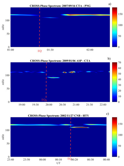
Figure 1. The cross-phase dynamical spectrograms between two low-latitude ground stations near the earthquake epicenter: panel (a) Sumatra 16 September 2009 EQ; panel (b) Indonesia 6 January 2009 EQ; panel (c) Philippines 11 November 2002 EQ. Each spectrum has been evaluated over a 1 h interval. Spectra have been smoothed both in time and frequency domains (7 frequency bands and 15 temporal bands). The red vertical line represents the earthquake occurrence time. In each panel the top caption reports the INTERMAGNET ground station codices used for the evaluation of the dynamical cross-phase spectrogram. The color-bar represents the phase difference in degrees between the equatorward and poleward ground magnetometer.

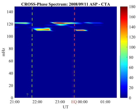
Figure 2. The cross-phase dynamical spectrograms for the Indonesia 11 September 2008 earthquake. Each spectrum has been evaluated over one hour interval. The spectra have been smoothed both in time and frequency domains (7 frequency bands and 15 temporal bands). The red vertical line represents the earthquake occurrence time. The green dashed line shows the occurrence of

f^{*}

decrease ∼2 h before the EQ main shock. The top caption reports the INTERMAGNET ground station codices used for the evaluation of the dynamical cross-phase spectrogram. The color-bar represents the phase difference in degrees between the equatorward and poleward ground magnetometer.

As expected, at low latitudes the FLR eigenfrequency is around 110 mHz [19,22,23]. For each event,

2 \pm 1

min after the earthquake occurrence (red dashed vertical line) there is a clear decrease of

f^{*}

. In fact, the upper (a), the middle (b) and the lower panels (c) show variations of ∼−10 mHz, ∼

- 25

mHz and ∼

- 12

mHz, respectively. The time duration of such variation is ∼15 min for the first (panel a) and the third (panel c) event, and ∼30 min for the second event (panel b). It is worth highlighting here that in

97 %

the FLR frequency variation were characterized by a single decrease coincident with the EQ occurrence, while in the remaining

3 %

was featured by a double

f^{*}

reduction as reported in Figure 2. In fact, in addition to the decrease of the FLR eigenfrequency at the moment of the EQ occurrence (red dashed vertical line), a clear reduction of

f^{*}

is also visible less than two hours before (green vertical dashed line). The variation is of ∼

- 10

mHz both for the coseismic

f^{*}

decrease as well as for the precursor

f^{*}

decrease, while the time duration is ∼40 min for the precursor phenomenon and ∼25 min for the coseismic phenomenon.

Figure 3 shows the statistical analysis of the EQ events characterized by a FLR decrease in terms of frequency variation (

δ f

) and relative time duration (

δ T

). It can be easily seen that the typical

δ T

of the eigenfrequency decrease (panel a) is between 25 and 35 min. On the other hand,

δ f

on average shows variations of ∼10 mHz. Figure 3c) shows the probability density (d

P

) of

δ f

as a function of

δ T

. d

P

has been estimated constructing bivariate histograms and using a kernel density estimator (e.g., [24]) with the following bin sizes:

δ f

, 3 mHz;

δ T

, 3 min. It results that the co-seismic FLR eigenfrequency variation is characterized by a frequency decrease of

12 \pm 3

mHz and a time duration of

36 \pm 3

min.

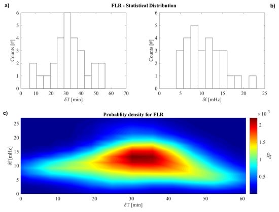
Figure 3. Eigenfrequency variation (panel (a)) and relative time duration (panel (b)) data distributions of the FLR. Panel (c) shows the probability density distribution of the eigenfrequency variation as a function of the relative time duration.

4. Discussion

In order to provide a quantitative explanation to the observed FLR eigenfrequency variations, we modelled the

f^{*}

behaviour during the occurrence of an EQ. It is well known that a geomagnetic field line, with both ends fixed in the ionosphere can be sketched as a string whose frequency depends on both the magnetic field geometry and the plasma density along the field line [19,21,25,26]. Following the approach of Singer et al. [27], we have evaluated

f^{*}

for an arbitrary magnetic field geometry, starting from the Magnetohydrodynamic (MHD) equations related to a stationary EM wave. By referring to the model reported in Appendix A, we have numerically solved the Equation (A8) using the magnetic equator as reference point

V_{A} (s_{0}) = V_{A} (e q)

(

V_{A}

being the Alfvén speed). We have used the IGRF (International Geomagnetic Reference Field) model [28] for the internal Earth’s magnetic field, the T01 model [29,30] for the external part of the Earth’s magnetic field and a radial power law dependence for the plasma mass density,

ρ / ρ_{e q} = {(r / r_{e q})}^{- 3}

[26]. The boundary conditions of fixed footpoints have been established at some level in the ionosphere, i.e., at

h = 120

km altitude corresponding to the E-layer, where the Alfvén wave is assumed to be perfectly reflected [17]. Finally, the values of the eigenfrequency

f^{☆}

have been obtained through Equation (A9) of Appendix A.

Figure 4 shows the modelled diurnal eigenfrequency behaviour of a field line footprinted at

λ_{m a g} = 20^{°}

(

λ_{m a g}

being the magnetic latitude). Around noon, we modified the plasma density at the footprint of the field line using a gradient pressure (

\nabla p_{d e n}

) which produces a density variation of

15 %

lasting for about 10 min. Such

\nabla p_{d e n}

is the result of the application of the M.I.L.C. model to an EQ characterized by a magnitude

M_{E Q} = 6.5

, a

P G A

= 0.6 g and a

Δ t

= 20 s (

P G A

and

Δ t

being the Peak Ground Acceleration and time duration of the EQ, respectively). The M.I.L.C. model is based on the assumption that an EQ creates an acoustic gravity wave, which propagates through the atmosphere. The pressure gradient induced by the AGW causes local instability in the ionospheric plasma density distribution, giving rise to both plasma and EM waves propagating up to the magnetosphere. In general, it is well known that the concurring contribution of the EM wave energy and/or of the plasma density variation produces a change in the local FLR eigen-frequency [19,31,32]. Indeed, Figure 4 shows that our model is able to produce a clear

f^{*}

collapse in correspondence to the plasma density gradient. This result is the consequence of Equation (A9) according to which any variation in the local magnetic field and/or in the local plasma density produces a corresponding change in

f^{*}

. It is important to remind here that the use of the IGRF and the T01 model in solving Equation (A8) produces a

5 %

maximum error in the evaluation of

f^{*}

[23].

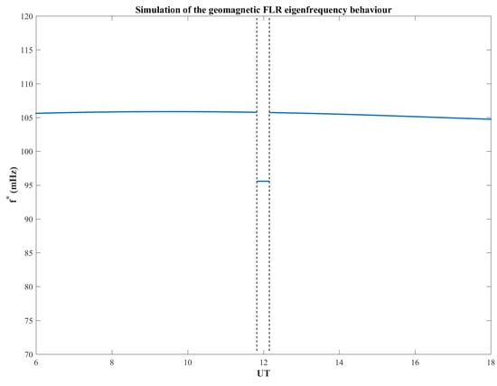
Figure 4. As an example, in the Figure, is shown the simulated behaviour of the FLR eigen-frequency obtained by our modeled for a potential EQ occurred at

20^{°}

magnetic latitude.

The result displayed in Figure 4 is consistent with the experimental FLR eigenfrequency behaviour detected in correspondence of an EQ. In fact, both Figure 1 and Figure 2 show a sudden decrease of

f^{*}

of ∼10 mHz,

2 \pm 1

min after the EQ occurrence lasting for 20–30 min. Such result completely agree with the probability density bi-variate distribution in Figure 3c). However, we need to stress here that at low magnetic latitudes (

0^{°} \leq λ_{m a g} \leq 30^{°}

) the geomagnetic field line is almost completely surrounded by the ionosphere. As a consequence any alteration in the ionospheric plasma density induces a variation in the corresponding eigenfrequency. Consequently, we do interpret the

f^{*}

changes observed in our 28 EQ events (see Table 1) as caused by the ionospheric plasma density variation induced by the emission of a co-seismic AGW leading to a pressure gradient [15].

Finally, in the case of the absence of a co-seismic AGW emission, no possible

f^{*}

variations can be detected (10 case event, see Table 1). Such a hypothesis is confirmed by Carbone et al. [15], showing that the atmospheric fluctuations excited by a generic seismic event on the top of the first layer of the atmosphere can be evanescent. In fact, depending on the characteristic parameters of the EQ (length of the fault, peak ground acceleration strong time duration and so on), a the propagation of the AGW up to the ionosphere can be prevented. In order to confirm such hypothesis, for these events, we analyzed the vertical atmospheric temperature profiles using the approach described in Piersanti et al. [16] to catch for possible AGW injection. Here, we display the analysis of the 19/12/2006 Sumatra EQ, since the remaining nine case events show similar results.

Figure 5a shows the atmospheric vertical temperature profile (T) as obtained from ERA5, which is the 5th generation atmospheric data set produced by the European Centre for Medium-Range Weather Forecasts [33]. The temperature fluctuations (

T^{'}

), evaluated as the difference between T and its 2 km moving average, show the expected minimum and maximum at the tropopause (∼18 km) and the stratopause [34], respectively. A similar behaviour can be found in both the

B r u n t - V \ddot{a} i s \ddot{a} l \ddot{a}

frequency (

N^{2}

) and the potential energy density (

E_{P}

) value [35]. The lack of any possible wave behaviour in

T^{'}

confirms the absence of AGW (and reference therein [36]) injected at the moment of the EQ occurrence. As a consequence, we can reasonably affirm that the missing of AGW prevents any possible variation of ionospheric plasma density distribution leading to the FLR eigenfrequency variation.

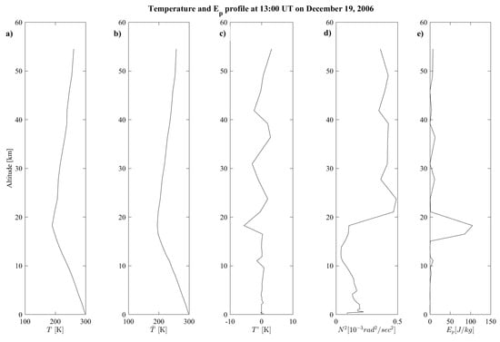
Figure 5. Example of AGW analysis. Vertical profiles of: (a) temperature; (b) background temperature; (c) temperature deviation, (d) square term of

B r u n t - V \ddot{a} i s \ddot{a} l \ddot{a}

frequency, and (e) potential energy at 13:00 UT on 19 December 2006.

Finally, it is worth noticing that the variation of

f^{*}

does not show any dependence on earthquake magnitude (not shown). Such result agrees with Carbone et al. [15], who demonstrated that the emission of a non-evanescent AGW, generating FLR variation, does not depend on the individual earthquake parameter alone, but on both the combination of the length of the fault, the PGA, the time duration of the EQ, etc (see dispersion relation in Carbone et al. [15]), and the local atmospheric scale height.

5. Conclusions

In the last 20 years, many investigations focused on the possible identification of magnetospheric perturbations directly connected to earthquake occurrence ([37] and reference therein). This paper presents the first evidence, via observation and modelling, of changes in magnetospheric FLR eigenfrequency associated to the EQ occurrence, demonstrating a causal connection between seismic phenomena and space based observables. We have analyzed more than 40 low latitudes EQ from 2000 to 2020, during quiet solar condition in order to search for magnetospheric signal associate to seismic activity. In 28 events, we found a clear sudden decrease of the magnetospheric FLR eigenfrequencies, while in 10 cases we did not find any

f^{*}

variation. The proposed explanation is that the plasma density at the footprint of the field line magnetically connected to the EQ location was modified of about

Δ ρ ≃ 15 %

, by a gradient pressure fluctuations

\nabla p_{d e n}

induced by a propagation of an AGW emitted during the EQ occurrence [15,16]. At low latitudes the magnetospheric field lines are fully surrounded by the ionosphere and the FLR eigenfrequencies, depending on both the magnetic field and the plasma density along the field line [19,31], is expected to decrease [23,26,32]. On the other hand, the possible explanation of the null

f^{*}

variation observed in 10 case events, can be found in the lack of the vertical propagation of the AGW (evanescent) up to the ionosphere, as predicted by the Carbone et al. [15] analytical model.

In is interesting to note that the FLR decrease observed in one case some hours before the EQ occurrence (Figure 2) could be due to various reasons, such as high-level seismic activity (especially for events characterized by a sequence of foreshocks before the main shocks), or to the outflow of radioactive gases (e.g., due to radon decay) by the Earth’s surface [37,38]. Indeed, both these phenomena would be able to generate changes in atmospheric temperature and hence AGW formation (e.g., [39]). A similar result was found in Piersanti et al. [16] who found a decrease of

f^{*}

5 h before the EQ occurrence. They explained their observation in terms of the M.I.L.C. model, pointing out that any AGW can produce a variation of the ionospheric plasma density distribution (such as travelling ionospheric disturbances [40]) which in turns changes the Alfvén velocity along the field line giving rise to a change of the FLR eigenfrequency [19].

In conclusion, our results confirm analytically the direct coupling among lithosphere, ionosphere and magnetosphere during active seismic conditions, supporting the models introduced by [16,37] and opening the way to new remote sensing methods combining space and ground sensing of the earth seismic activity.

Author Contributions

M.P. writing—original draft preparation, formal analysis, methodology, investigation and Conceptualization; W.J.B. writing—review and editing, methodology, investigation; V.C. writing—review and editing, validation; R.B. writing—review and editing, methodology and coordination; R.I. data curation and validation; P.U. writing—review and editing and project administration. All authors have read and agreed to the published version of the manuscript.

Funding

This research received no external funding.

Institutional Review Board Statement

Not applicable.

Informed Consent Statement

Not applicable.

Data Availability Statement

Ground geomagnetic observatory data are provided by INTERMAGNET (www.intermagnet.org, accessed on 16 July 2021), and SUPERMAG (https://supermag.jhuapl.edu), accessed on 16 July 2021; Earthquake parameters comes from USGS data catalog (https://earthquake.usgs.gov/), accessed on 16 July 2021.

Acknowledgments

The authors thank the national institutes that support INTERMAGNET for promoting high standards of the magnetic observatory practice (www.intermagnet.org, accessed on 14 July 2021). The authors thank the provision of magnetometer data from SUPERMAG (https://supermag.jhuapl.edu, accessed on 14 July 2021). The parameters of the earthquake are provided by USGS data catalog (https://earthquake.usgs.gov/, accessed on 14 July 2021). M. Piersanti, R. Battiston and R. Iuppa thank the Italian Space Agency for the financial support under the contract ASI “LIMADOU Scienza+” n

^{°}

2020-31-HH.0. M. Piersanti thanks the ISSI-BJ project “The electromagnetic data validation and scientific application research based on CSES satellite” and Dragon 5 cooperation 2020-2024 (ID. 59236).

Conflicts of Interest

The authors declare no conflict of interest.

Abbreviations

The following abbreviations are used in this manuscript:

AGW	Acoustic Gravity Wave
EM	Electromagnetic
EQ	Earthquake
FLR	Field Line Resonance
IGRF	International Geomagnetic Reference Field
MHD	Magnetohydrodynamic
M.I.L.C.	Magnetosphere Ionosphere Lithosphere Coupling
VLF	Very Low Frequency

Appendix A. Field Line Resonance Eigenfrequency Equation

The external perturbation pressure

δ P_{A G W}

produced by the AGW, impinging on the ionospheric plasma from below, is able to modify the density field thus inducing a dynamics of plasma which, in turns, produces a perturbed magnetic field

b = B - B_{0}

of the background magnetic field

B_{0}

. As an order of magnitude estimate, from the Ampere law

| \nabla b | \sim β \nabla δ ρ

, being

δ ρ

the fluctuating density and

β

is the plasma parameter. As a consequence, by using a relation between density and pressure fluctuation, for example the adiabatic gas law, it can be found

| \nabla b | \sim (β ρ_{0}^{2} / γ P_{0} B_{0}) \nabla δ P_{A G W}

, being

ρ_{0}

and

P_{0}

some reference values for density and pressure, and

γ

is the adiabatic index.

The corresponding low-frequency dynamics of the plasma can be roughly described by the ideal dissipationless MHD equations

\begin{matrix} ρ [\frac{\partial v}{\partial t} + (v \cdot \nabla) v] & = & j \times B - \nabla P \\ \frac{\partial B}{\partial t} & = & \nabla \times E \end{matrix}

(A1)

where

v

is the fluctuation velocity,

j

the current density,

E

the electric field fluctuations and P the internal pressure. The electric field fluctuations can be obtained by the Ohm’s law by neglecting the Hall term and the electron pressure gradient because we are interested at the low-frequency evolution of plasma corresponding to scales much greater than the Larmor radius, so that

E = - v \times B

. Furthermore, we are dealing with a low-

β

plasma [41], so that dynamical processes occurring within the ionospheric plasma cannot significant alter the background magnetic field, so that the internal pressure gradient

\nabla P

can be neglected in the momentum Equation (A1). It is worthwhile to note that the same approximations are usually used to describe the plasma dynamics of low-

β

laboratory plasma, for example confined in Reversed Field Pinch devices (e.g., [42]).

To model the eigenfrequencies

f^{*}

and amplitudes of low-frequency transverse waves, we use a linear model from Equation (A1), which describes the linear dynamics of fluctuations, namely

\begin{matrix} ρ_{0} μ_{0} \frac{\partial v}{\partial t} & ≃ & (\nabla \times b) \times B_{0} \\ \frac{\partial b}{\partial t} & ≃ & \nabla \times (v \times B_{0}) \end{matrix}

(A2)

where we used the Ampere’s law

\nabla \times B = μ_{0} j

. Note that, by considering the plasma dynamics generated by AGW, the perturbed magnetic field can be viewed as generated by a small displacement

ξ

of the plasma [43], not by a compression of the field lines, so that

b

lye along the field line and produces the force in the momentum equation. The linear model (A2) neglects the background current density

j_{0}

related to the background magnetic field [29,30]. In fact, as an order of magnitude estimate, the background current density

| j_{0} | ≃ 1.8 \times 10^{- 10}

A/m

^{2}

results ten times lower than the current density

| j | \sim b / l_{‖} ≃ 10^{- 9}

A/m

^{2}

(

l_{‖}

is the scale length along the fluctuating magnetic field direction). Let us consider a geometry where the z-axis is directed between the field lines. However, both footpoints of a field line are fixed in the ionosphere, so that the displacement and the separation of adjacent lines can be described by a function

h (x, y, z)

. From the last Equation (A2), using

v = \partial ξ / \partial t

along the z-direction, we get the perturbed magnetic field

b = \nabla \times (ξ e_{z} \times B_{0})

(A3)

(being

e_{z}

the unit vector in the direction z) apart from a constant which can be cast to zero without losing generality. Then, from the momentum equation we obtain a relation for the displacement along the z direction

ρ_{0} μ_{0} \frac{\partial^{2} ξ}{\partial t^{2}} = (B_{0} \cdot \nabla) [(B_{0} \cdot \nabla) ξ]

(A4)

By introducing the Alfvén velocity

V_{A} = B_{0} / \sqrt{ρ_{0} μ_{0}}

and the normalized displacement

ξ^{'} = ξ / h

we finally obtain the wave equation for the displacement

\frac{\partial^{2} ξ^{'}}{\partial t^{2}} = V_{A}^{2} (e_{0} \cdot \nabla) [h (e_{0} \cdot \nabla) ξ^{'} + ξ^{'} (e_{0} \cdot \nabla) h]

(A5)

where

e_{0}

represents the unit vector along the background magnetic field.

If we consider now the ansatz where

ξ^{'}

behaves as

e^{i ω t}

, under the hypothesis that the field curvature is smooth enough so the function h is slowly variable, from Equation (A5) we obtain

(e_{0} \cdot \nabla) [(e_{0} \cdot \nabla) ξ^{'}] + [(e_{0} \cdot \nabla) ln h^{2}] [(e_{0} \cdot \nabla) ξ^{'}] + \frac{ω^{2}}{V_{A}^{2}} ξ^{'} ≃ 0

(A6)

Introducing the coordinate s along the field line

(e_{0} \cdot \nabla) = ℓ^{- 1} \partial / \partial s

, where ℓ is the characteristic length of the field line between two ionospheric footpoints, say using the coordinate system where

0 \leq s \leq 1

, we obtain the characteristic value wave equation

\frac{\partial^{2} ξ^{'}}{\partial s^{2}} + P (s) \frac{\partial ξ^{'}}{\partial s} + (\frac{ω^{2} ℓ^{2}}{V_{A}^{2}}) ξ^{'} = 0

(A7)

being

P (s) = \partial ln h^{2} / \partial s

, a unknown function which depends on the coordinate along the field line. The characteristic frequencies

f^{☆}

we are looking for, correspond to the characteristic values

ω

, which can be obtained once the Sturm-Liouville Equation (A7) is solved supplied by appropriate boundary conditions, for example the condition of fixed footpoints

ξ^{'} (s_{☆}) = {(\partial ξ^{'} / \partial s)}_{s = s_{☆}} = 0

at both

s_{☆} = 0, 1

.

To solve the characteristic value equation we can introduce a unknown eigenvalue

λ

by modifying the equation as

\frac{\partial^{2} ξ^{'}}{\partial s^{2}} + P (s) \frac{\partial ξ^{'}}{\partial s} + λ [\frac{V_{A}^{2} (s_{0})}{V_{A}^{2} (s)}] ξ^{'} = 0

(A8)

where

V_{A} (s_{0})

is the value of the Alfvén speed in a point

s_{0}

. The solution of Equation (A8) gives us the eigenvalue

λ

compatible with both the boundary conditions and a fixed value of

V_{A} (s_{0})

. Finally, by a comparison of (A7) and (A8), the characteristic frequencies results to be

f^{☆} = \frac{V_{A}^{2} (s_{0}) \sqrt{λ}}{ℓ}

(A9)

It can be possible to analytically solve Equation (A8) for some particular geometries, by making explicit the function

P (s)

and estimate the value of

V_{A} (s_{0})

. For example in a dipole field the azimuthal field line displacement, is proportional to

h ≃ r sin θ

[27], corresponding to a toroidal mode. However, we aimed to a direct comparison with real observations of the eigenfrequencies

f^{☆}

, and this necessarily requires a numerical integration of Equation (A8), because we need the exact knowledge of the function

P (s)

.

References

Gokhberg, M.B.; Morgounov, V.A.; Yoshino, T.; Tomizawa, I. Experimental measurement of electromagnetic emissions possibly related to earthquakes in Japan. J. Geophys. Res. 1982, 87, 7824–7828. [Google Scholar] [CrossRef]
Gokhberg, M.B.; Pilipenko, V.A.; Pokhotelov, O.A. On the seismic precursors within the ionosphere. Izv. Acad. Sci. USSR Ser. Physics Earth 1983, 10, 17–21. [Google Scholar]
Larkina, V.I.; Nalivayko, A.V.; Gershenzon, N.I.; Gokhberg, M.B.; Liperovskiy, V.A.; Shalimov, S.L. Observation of VLF emission related with seismic activity on the Intercosmos-19 satellite. Geomagn. Aeron. 1993, 23, 684–687. [Google Scholar]
Battiston, R.; Vitale, V. First evidence for correlations between electron fluxes measured by NOAA-POES satellites and large seismic events. Nucl. Phys. B Proc. Suppl. 2013, 243–244, 249–257. [Google Scholar] [CrossRef]
Sgrigna, V.; Carota, L.; Conti, L.; Corsi, M.; Galper, A.M.; Koldashov, S.V.; Murashov, A.M.; Picozza, P.; Scrimaglio, R.; Stagni, L. Correlations between earthquakes and anomalous particle bursts from SAMPEX/PET satellite observations. J. Atmos. Sol. Terr. Phys. 2005, 67, 1448–1462. [Google Scholar] [CrossRef]
Molchanov, O.; Rozhnoi, A.; Solovieva, M.; Akentieva, O.; Berthelier, J.J.; Parrot, M.; Lefeuvre, F.; Biagi, P.F.; Castellana, L.; Hayakawa, M. Global diagnostics of the ionospheric perturbations related to the seismic activity using the VLF radio signals collected on the DEMETER satellite. Nat. Hazard Earth Sys. 2006, 6, 745–753. [Google Scholar] [CrossRef]
Bertello, I.; Piersanti, M.; Candidi, M.; Diego, P.; Ubertini, P. Electromagnetic field observations by the DEMETER satellite in connection with the L’Aquila earthquake. Ann. Geophys. 2018, 36, 1483–1493. [Google Scholar] [CrossRef] [Green Version]
Gokhberg, M.B.; Kustov, A.V.; Liperovsky, V.A.; Liperovskaya, R.K.; Kharin, E.P.; Shalimov, S.L. About disturbances in F-region of ionosphere before strong earth-quakes. Izvestiya Acad. Sci. USSR Ser. Physics Earth 1988, 4, 12–20. [Google Scholar]
Fraser-Smith, A.C.; Bernardi, A.; McGill, P.R.; Ladd, M.; Helliwell, R.; Villard, O.G., Jr. Low-frequency magnetic field measurements near the epicenter of the Ms 7.1 Loma Prieta earthquake. Geophys. Res. Lett. 1990, 17, 1465–1468. [Google Scholar] [CrossRef]
Gogatishvili, I.M. Geomagnetic precursors of intense earthquakes in the spectrum of geomagnetic pulsations with frequencies of 1–0.02 Hz. Geomagn. Aeron. 1984, 24, 697–700. [Google Scholar]
Kolokolov, L.E.; Liperovskaya, E.V.; Liperovsky, V.A.; Pokhotelov, O.A.; Mararovsky, A.V.; Shalimov, S.L. Sudden diffusion of sporadic E-layers in the mid-latitude ionosphere during the earthquake preparation. Izvestiya RAN Earth Phys. 1992, 7, 105–113. [Google Scholar]
Parrot, M. Statistical study of ELF/VLF emissions recorded by a low-altitude satellite during seismic events. J. Geophys. Res. 1994, 99, 23339. [Google Scholar] [CrossRef]
Serebryakova, O.N.; Bilichenko, S.V.; Chmyrev, V.M.; Parrot, M.; Ranch, J.L.; Lefeuvre, F.; Pokhotelov, O.A. Electromagnetic ELF radiation from earthquakes regions as observed by low-altitude satellites. Geophys. Res. Lett. 1992, 19, 91. [Google Scholar] [CrossRef]
Migulin, V.V.; Larkina, V.I.; Molchanov, O.A.; Nalivaiko, A.V.; Gokhberg, M.B.; Pilipenko, V.A.; Liperovsky, V.A.; Pokhotelov, O.A.; Shalimov, S.L. Detection of earthquake influence on the ELF/VLF emissions at the upper ionosphere. Preprint IZMIRAN 1982, 25, 2390. [Google Scholar]
Carbone, V.; Piersanti, M.; Materassi, M.; Battiston, R.; Lepreti, F.; Ubertini, P. A mathematical model of Lithosphere-Atmospherecoupling for seismic events. Sci. Rep. Nat. 2021. [Google Scholar] [CrossRef]
Piersanti, M.; Materassi, M.; Battiston, R.; Carbone, V.; Cicone, A.; D’Angelo, G.; Diego, P.; Ubertini, P. Magnetospheric–Ionospheric–Lithospheric Coupling Model. 1: Observations during the 5 August 2018 Bayan Earthquake. Remote Sens. 2020, 12, 3299. [Google Scholar] [CrossRef]
Waters, C.L.; Menk, F.W.; Fraser, B.J. Low latitude geomagnetic field line resonances: Experiment and modeling. J. Geophys. Res. 1994, 99, 547. [Google Scholar] [CrossRef]
Green, A.W.; Worthington, E.W.; Baransky, L.N.; Fedorov, E.N.; Kurneva, N.A.; Pilipenko, V.A.; Shvetzov, D.N.; Bektemirov, A.A.; Philipov, G.V. Alfven field line resonances at low latitudes (L = 1.5). J. Geophys. Res. 1993, 98, 15693–15699. [Google Scholar] [CrossRef]
Waters, C.L.; Samson, J.C.; Donovan, E.F. Variation of plasmatrough density derived from magnetospheric field line resonances. J. Geophys. Res. 1996, 101, 24737–24745. [Google Scholar] [CrossRef]
Matzka, J.; Bronkalla, O.; Tornow, K.; Elger, K.; Stolle, C. Geomagnetic Kp index. V. 1.0. GFZ Data Services. 2021. Available online: https://dataservices.gfz-potsdam.de/panmetaworks/showshort.php?id=escidoc:5216888 (accessed on 16 July 2021). [CrossRef]
Menk, F.W.; Waters, C.L. Magnetoseismology: Ground-Based Remote Sensing of Earth’s Magnetosphere; Wiley: Hoboken, NJ, USA, 2013. [Google Scholar]
Menk, F.W.; Waters, C.L.; Fraser, B.J. Field line resonances and waveguide modes at low latitudes: 1. Observations. J. Geophys. Res. 2000, 105, 7747–7761. [Google Scholar] [CrossRef]
Vellante, M.; Piersanti, M.; Pietropaolo, E. Comparison of equatorial plasma mass densities deduced from field line resonances observed at ground for dipole and IGRF models. J. Geophys. Res. 2014, 119. [Google Scholar] [CrossRef]
Martinez, W.L.; Martinez, A.R. Computational Statistics Handbook with MATLAB; Chapman and Hall/CRC: Boca Raton, FL, USA, 2002. [Google Scholar]
Rankin, R.; Tikhonchuk, V.T. Dispersive shear Alfvén waves on model Tsyganenko magnetic field lines. Adv. Space Res. 2001, 28, 1595. [Google Scholar] [CrossRef]
Vellante, M.; Piersanti, M.; Heilig, B.; Reda, J.; Corpo, A.D. Magnetospheric plasma density inferred from field line resonances: Effects of using different magnetic field models. In Proceedings of the 2014 XXXIth URSI General Assembly and Scientific Symposium (URSI GASS), Beijing, China, 16–23 August 2014; pp. 1–4. [Google Scholar] [CrossRef]
Singer, H.J.; Southwood, D.J.; Walker, R.J.; Kivelson, M.G. Alfven wave resonances in a realistic magnetospheric magnetic field geometry. J. Geophys. Res. 1981, 86, 4589. [Google Scholar] [CrossRef] [Green Version]
Thébault, E.; Finlay, C.C.; Beggan, C.D.; Alken, P.; Aubert, J.; Barrois, O.; Bertr, F.; Bondar, T.; Boness, A.; Brocco, L.; et al. International Geomagnetic Reference Field: The 12th generation. Earth Planet Sp. 2015, 67, 79. [Google Scholar] [CrossRef]
Tsyganenko, N.A. A model of the magnetosphere with a dawn-dusk asymmetry, 1, Mathematical structure. J. Geophys. Res. 2002, 107. [Google Scholar] [CrossRef] [Green Version]
Tsyganenko, N.A. A model of the near magnetosphere with a dawn-dusk asymmetry, 2, Parameterization and fitting to observations. J. Geophys. Res. 2002, 107. [Google Scholar] [CrossRef]
Menk, F.W.; Kale, Z.; Sciffer, M.; Robinson, P.; Waters, C.L.; Grew, R.l.; Clilverd, M.; Mann, I. Remote sensing the plasmasphere, plasmapause, plumes and other features using ground-based magnetometers. J. Space Weather Space Clim. 2014, 4, A34. [Google Scholar] [CrossRef] [Green Version]
Piersanti, M.; Villante, U.; Waters, C.; Coco, I. The 8 June 2000 ULF wave activity: A case study. J. Geophys. Res. 2012, 117. [Google Scholar] [CrossRef] [Green Version]
Hennermann, K. ERA5 Data Documentation. In Copernicus Knowledge Base. 2017. Available online: https://confluence.ecmwf.int/display/CKB/ERA5+data+documentation (accessed on 19 October 2017).
Tsuda, T.; Murayama, Y.; Nakamura, T.; Vincent, R.A.; Manson, A.H.; Meek, C.E.; Wilson, R.L. Variations of the gravity wave characteristics with height, season and latitude revealed by comparative observations. J. Atmos. Terr. Phys. 1994, 56, 555–568. [Google Scholar] [CrossRef]
Tsuda, T.; Nishida, M.; Rocken, C.; Ware, R.H. A global morphology of gravity wave activity in the stratosphere revealed by the GPS occultation data (GPS/MET). J. Geophys. Res. 2000, 105, 7257–7273. [Google Scholar] [CrossRef]
Yang, S.-S.; Asano, T.; Hayakawa, M. Abnormal gravity wave activity in the stratosphere prior to the 2016 Kumamoto earthquakes. J. Geophys. Res. Space Phys. 2019, 124. [Google Scholar] [CrossRef]
Pulinets, S.A.; Ouzounov, D.P. Lithosphere–atmosphere–ionosphere coupling (LAIC) model—An unified concept for earthquake precursors validation. J. Asian Earth Sci. 2011, 41, 371–382. [Google Scholar] [CrossRef]
Hayakawa, M.; Kasahara, Y.; Nakamura, T.; Hobara, Y.; Rozhnoi, A.; Solovieva, M.; Molchanov, O.; Korepanov, V. Atmospheric gravity waves as a possible candidate for seismo-ionospheric perturbation. J. Atmo. Electr. 2011, 31, 129–140. [Google Scholar] [CrossRef] [Green Version]
Hayakawa, M.; Kasahara, Y.; Nakamura, T.; Muto, F.; Horie, T.; Maekawa, S.; Hobara, Y.; Rozhnoi, A.A.; Solovieva, M.; Molchanov, O.A. A statistical study on the correlation between lower ionospheric perturbations as seen by subionospheric VLF/LF propagation and earthquakes. J. Geophys. Res. 2010, 115, A09305. [Google Scholar] [CrossRef]
Hocke, K.; Schlegel, K. A review of atmospheric gravity waves and travelling ionospheric disturbances. Ann. Geophys. 1996, 14, 1996. [Google Scholar] [CrossRef]
Stubbe, P.; Hagfors, T. The Earth’s ionosphere: A wall-less plasma laboratory. Surv. Geophys. 1997, 18, 57–127. [Google Scholar] [CrossRef]
Cappello, S.; Escande, D.F. Bifurcation in viscoelastic MHD: The Hartmann Number and the Reversed Field Pinch. Phys. Rev. Lett. 2000, 85, 3838–3841. [Google Scholar] [CrossRef]
Cummings, W.D.; O’Sullivan, R.J.; Coleman, P.J. Standing Alfvén waves in the magnetosphere. J. Geophys. Res. 1969, 74, 778–793. [Google Scholar] [CrossRef]

Figure 1. The cross-phase dynamical spectrograms between two low-latitude ground stations near the earthquake epicenter: panel (a) Sumatra 16 September 2009 EQ; panel (b) Indonesia 6 January 2009 EQ; panel (c) Philippines 11 November 2002 EQ. Each spectrum has been evaluated over a 1 h interval. Spectra have been smoothed both in time and frequency domains (7 frequency bands and 15 temporal bands). The red vertical line represents the earthquake occurrence time. In each panel the top caption reports the INTERMAGNET ground station codices used for the evaluation of the dynamical cross-phase spectrogram. The color-bar represents the phase difference in degrees between the equatorward and poleward ground magnetometer.

Figure 2. The cross-phase dynamical spectrograms for the Indonesia 11 September 2008 earthquake. Each spectrum has been evaluated over one hour interval. The spectra have been smoothed both in time and frequency domains (7 frequency bands and 15 temporal bands). The red vertical line represents the earthquake occurrence time. The green dashed line shows the occurrence of

f^{*}

decrease ∼2 h before the EQ main shock. The top caption reports the INTERMAGNET ground station codices used for the evaluation of the dynamical cross-phase spectrogram. The color-bar represents the phase difference in degrees between the equatorward and poleward ground magnetometer.

Figure 3. Eigenfrequency variation (panel (a)) and relative time duration (panel (b)) data distributions of the FLR. Panel (c) shows the probability density distribution of the eigenfrequency variation as a function of the relative time duration.

Figure 4. As an example, in the Figure, is shown the simulated behaviour of the FLR eigen-frequency obtained by our modeled for a potential EQ occurred at

20^{°}

magnetic latitude.

Figure 5. Example of AGW analysis. Vertical profiles of: (a) temperature; (b) background temperature; (c) temperature deviation, (d) square term of

B r u n t - V \ddot{a} i s \ddot{a} l \ddot{a}

frequency, and (e) potential energy at 13:00 UT on 19 December 2006.

Table 1. Characteristics of the EQ events analyzed from 2001 to 2020. The X indicates a FLR eigenfrequency variation. The - indicates the absence of a FLR eigenfrequency variation. The NA indicates the impossibility to evaluate the FLR eigenfrequency. M is the earthquake magnitude. The parameters of the earthquake are provided by USGS data catalog (https://earthquake.usgs.gov/, accessed on: 16 July 2021).

FLR	Date	UTC Time	$K_{p}$	M	Latitude	Longitude	Region
X	17/07/2001	14.50.57	0	6.3	3.061 $^{°}$ S	148.180 $^{°}$ E	Bismarck Sea
X	27/11/2002	00.17.20	1	5.4	12.279 $^{°}$ N	120.753 $^{°}$ E	Philippines
X	12/12/2003	08.07.30	1	5.2	0.110 $^{°}$ S	123.991 $^{°}$ E	Indonesia
X	28/01/2004	07.41.04	1	5.7	4.931 $^{°}$ S	153.584 $^{°}$ E	New Guinea
-	09/02/2006	05.44.30	2	6.2	4.810 $^{°}$ S	133.063 $^{°}$ E	Indonesia
X	17/05/2006	01.21.26	1	6.0	3.743 $^{°}$ S	144.305 $^{°}$ E	New Guinea
X	24/06/2006	00.03.07	1	6.3	3.071 $^{°}$ S	127.183 $^{°}$ E	Indonesia
X	16/09/2007	01.20.38	2	6.4	2.763 $^{°}$ S	101.106 $^{°}$ E	Indonesia
-	26/10/2007	16.34.47	0	6.0	3.271 $^{°}$ S	143.763 $^{°}$ E	New Guinea
X	14/11/2007	17.44.04	2	5.7	23.215 $^{°}$ S	70.526 $^{°}$ W	Chile
-	25/07/2008	20.11.07	1	6.5	5.808 $^{°}$ S	146.658 $^{°}$ E	New Guinea
X	11/09/2008	00.00.02	1	6.6	1.885 $^{°}$ N	127.363 $^{°}$ E	Indonesia
-	19/12/2008	00.34.58	2	6.8	20.372 $^{°}$ N	146.339 $^{°}$ E	Mariana Islands
X	06/01/2009	19.56.25	2	6.0	0.566 $^{°}$ S	132.784 $^{°}$ E	Indonesia
X	16/02/2009	00.33.36	2	6.1	3.664 $^{°}$ S	149.608 $^{°}$ E	Bismarck Sea
X	02/03/2009	00.03.39	1	6.5	1.105 $^{°}$ S	119.868 $^{°}$ E	Indonesia
X	25/07/2009	18.41.58	2	5.8	1.869 $^{°}$ N	97.020 $^{°}$ E	Indonesia
X	15/10/2009	03.34.28	1	6.0	1.111 $^{°}$ N	85.322 $^{°}$ W	Ecuador
-	24/02/2008	04.36.29	2	6.5	3.741 $^{°}$ S	101.986 $^{°}$ E	Indonesia
NA	07/06/2008	19.10.48	2	5.0	3.552 $^{°}$ S	140.851 $^{°}$ E	Indonesia
-	02/07/2008	00.08.31	2	5.2	12.451 $^{°}$ N	44.202 $^{°}$ W	Mid-Atlantic
X	07/02/2008	23.16.41	1	5.3	17.558 $^{°}$ N	144.922 $^{°}$ E	Mariana Islands
-	19/12/2006	12.48.16	2	6.0	2.458 $^{°}$ N	98.000 $^{°}$ E	Idonesia
X	16/11/2009	18.34.24	0	5.2	19.556 $^{°}$ S	70.365 $^{°}$ W	Chile
NA	11/01/2009	14.03.49	1	5.6	6.388 $^{°}$ S	147.423 $^{°}$ E	New Guinea
NA	11/01/2009	14.15.54	1	5.0	0.769 $^{°}$ S	133.506 $^{°}$ E	Indonesia
X	16/09/2008	21.47.14	2	5.7	17.438 $^{°}$ N	73.915 $^{°}$ E	India
X	24/05/2003	01.46.06	1	5.9	14.428 $^{°}$ N	53.813 $^{°}$ E	Owen region
-	14/11/2007	18.55.49	2	5.1	22.670 $^{°}$ S	70.292 $^{°}$ W	Chile
NA	26/10/2007	16.34.47	1	5.6	3.271 $^{°}$ S	143.7630 E	New Guinea
X	22/11/2003	09.30.03	1	5.1	13.281 $^{°}$ N	57.466 $^{°}$ E	Arabic Sea
X	12/03/2008	01.32.34	2	6.0	1.934 $^{°}$ N	132.519 $^{°}$ E	Indonesia
X	02/02/2013	14.17.33	1	6.9	42.8 $^{°}$ N	143.27 $^{°}$ E	Japan
-	25/10/2013	17.10.16	2	7.1	37.194 $^{°}$ N	144.66 $^{°}$ E	Japan
X	06/10/2017	07.59.32	1	6.2	37.325 $^{°}$ N	144.02 $^{°}$ E	Japan
X	08/01/2019	12.39.31	2	6.3	30.526 $^{°}$ N	131.113 $^{°}$ E	Japan
X	18/06/2019	13.22.22	0	6.4	38.563 $^{°}$ N	139.504 $^{°}$ E	Japan
X	27/07/2019	18.31.07	1	6.3	33.015 $^{°}$ N	137.413 $^{°}$ E	Japan
X	19/04/2020	20.39.08	2	6.3	38.858 $^{°}$ N	141.99 $^{°}$ E	Japan
-	21/11/2016	20.58.47	1	6.9	38.296 $^{°}$ N	141.642 $^{°}$ E	Japan
X	05/08/2018	11.58.00	0	6.5	8.28 $^{°}$ S	116.4 $^{°}$ E	Indonesia
X	25/04/2015	06.45.21	2	6.6	28.18 $^{°}$ N	84.72 $^{°}$ E	Nepal

Publisher’s Note: MDPI stays neutral with regard to jurisdictional claims in published maps and institutional affiliations.

© 2021 by the authors. Licensee MDPI, Basel, Switzerland. This article is an open access article distributed under the terms and conditions of the Creative Commons Attribution (CC BY) license (https://creativecommons.org/licenses/by/4.0/).

On the Geomagnetic Field Line Resonance Eigenfrequency Variations during Seismic Event

Abstract

1. Introduction

2. Data and Methods

3. FLR Frequency Behaviour during Seismic Events

4. Discussion

5. Conclusions

Author Contributions

Funding

Institutional Review Board Statement

Informed Consent Statement

Data Availability Statement

Acknowledgments

Conflicts of Interest

Abbreviations

Appendix A. Field Line Resonance Eigenfrequency Equation

References

Article Metrics

Citations

Article Access Statistics