
DSMNN-Net: A Deep Siamese Morphological Neural Network Model for Burned Area Mapping Using Multispectral Sentinel-2 and Hyperspectral PRISMA Images


Abstract
:1. Introduction
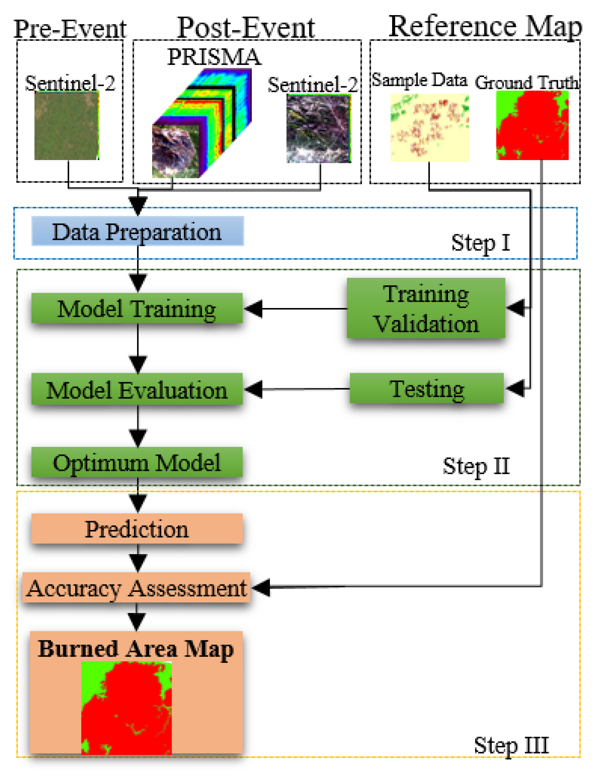
2. Methodology
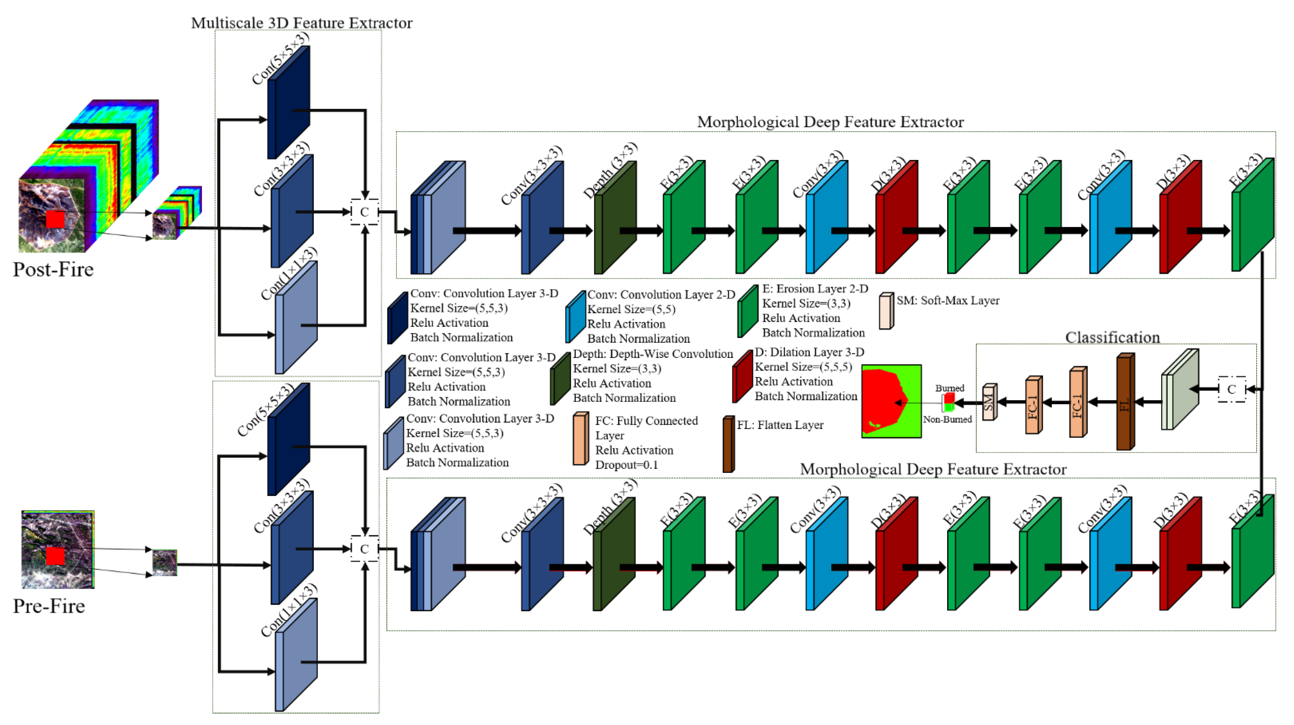
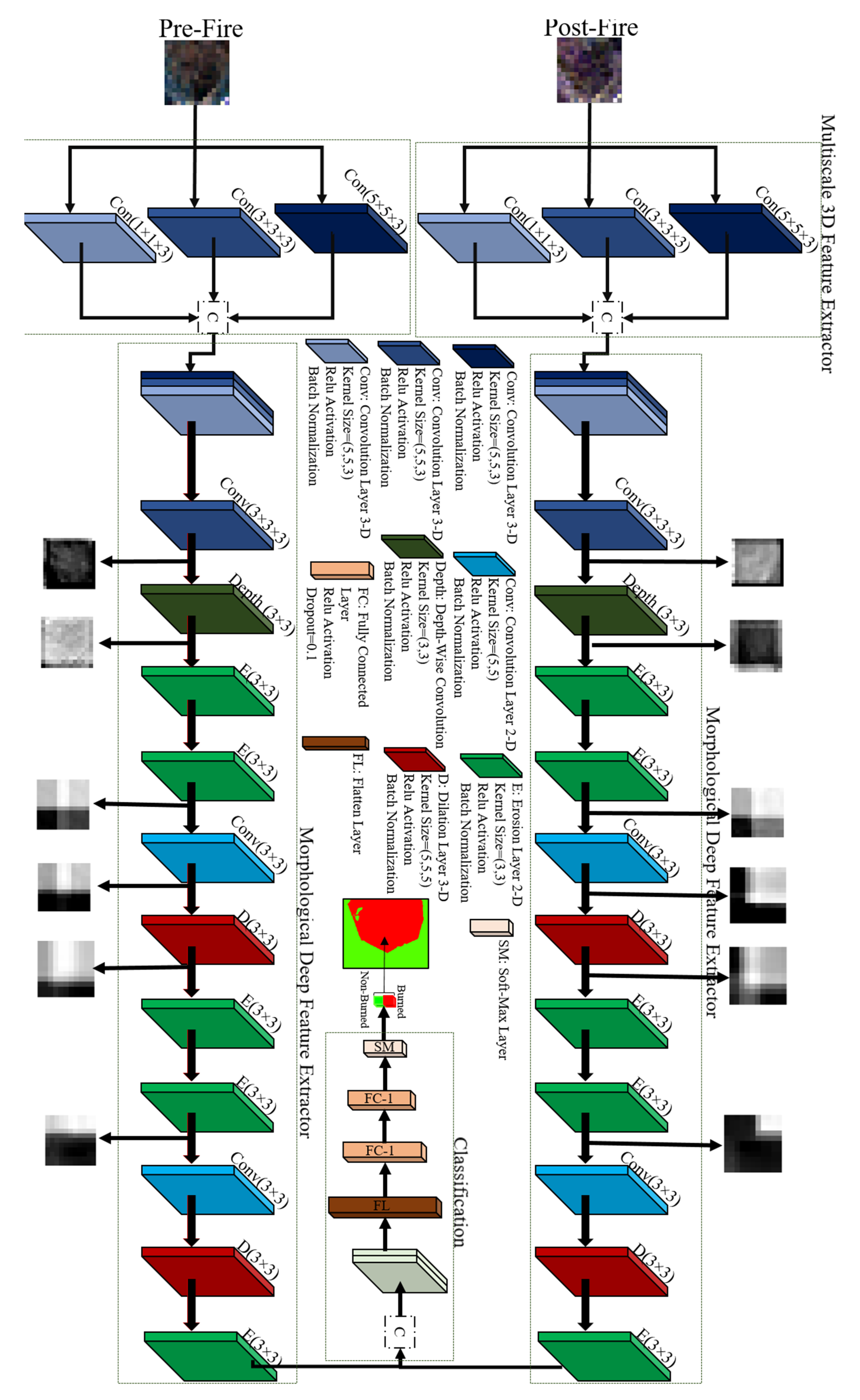
2.1. Proposed Deep Learning Architecture
2.2. Deep-Feature Extraction
- (1)
- We take advantage of multiscale convolution layers that increase the robustness of the network against the scale of variations.
- (2)
- We use the trainable morphological layers, which can increase the efficiency of the network for the extraction of nonlinear features.
- (3)
- We use 3D convolution layers to make use of the full content of the spectral information in the hyperspectral and multispectral datasets.
- (4)
- We use depthwise convolution layers that are computationally cheaper and can help to reduce the number of parameters and to prevent overfitting.
2.3. Convolution Layer
2.4. Morphological Operation Layers
2.5. Classification
2.6. Training Process
2.7. Accuracy Assessment
3. Case Study and Satellite Images
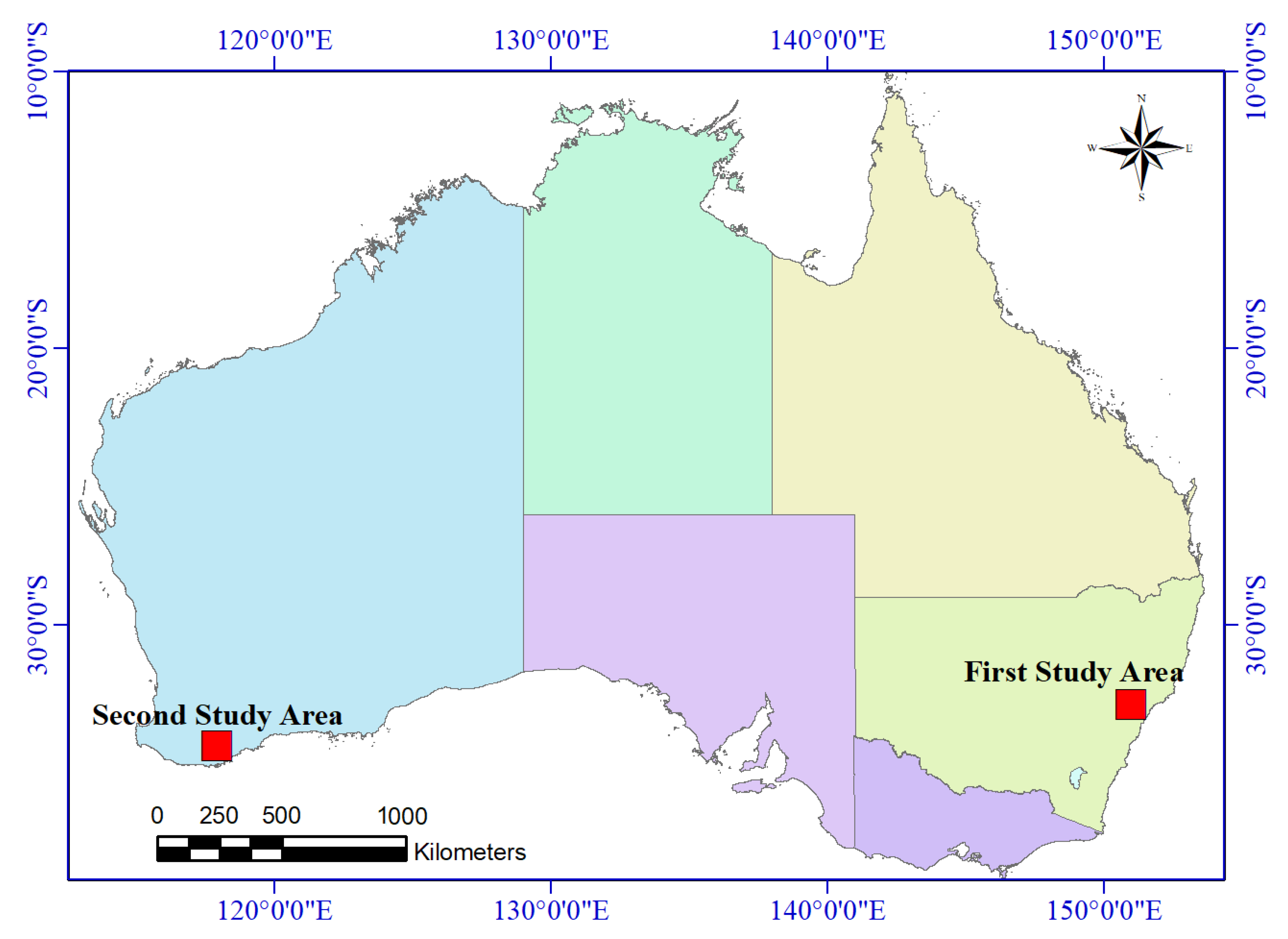
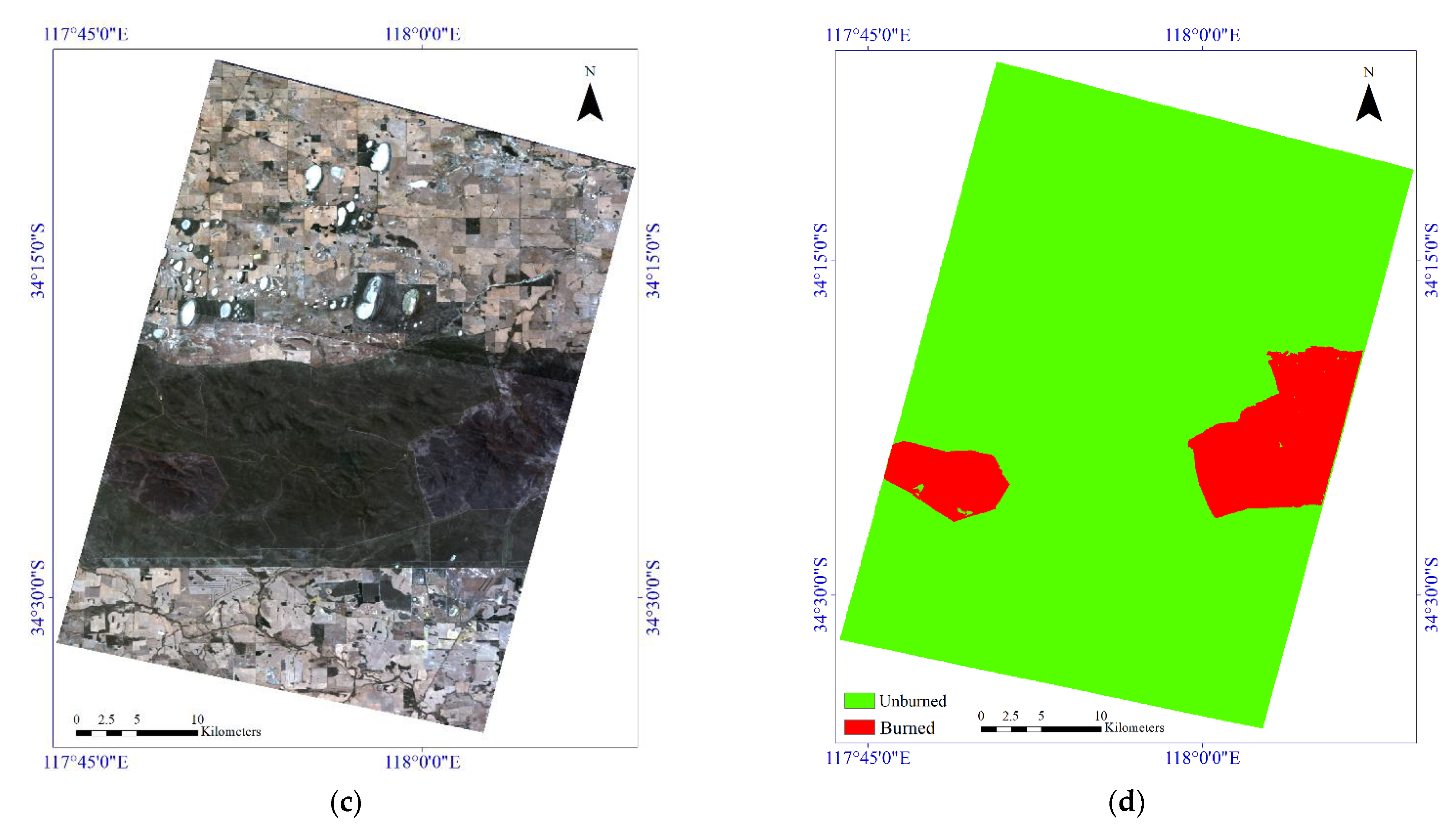
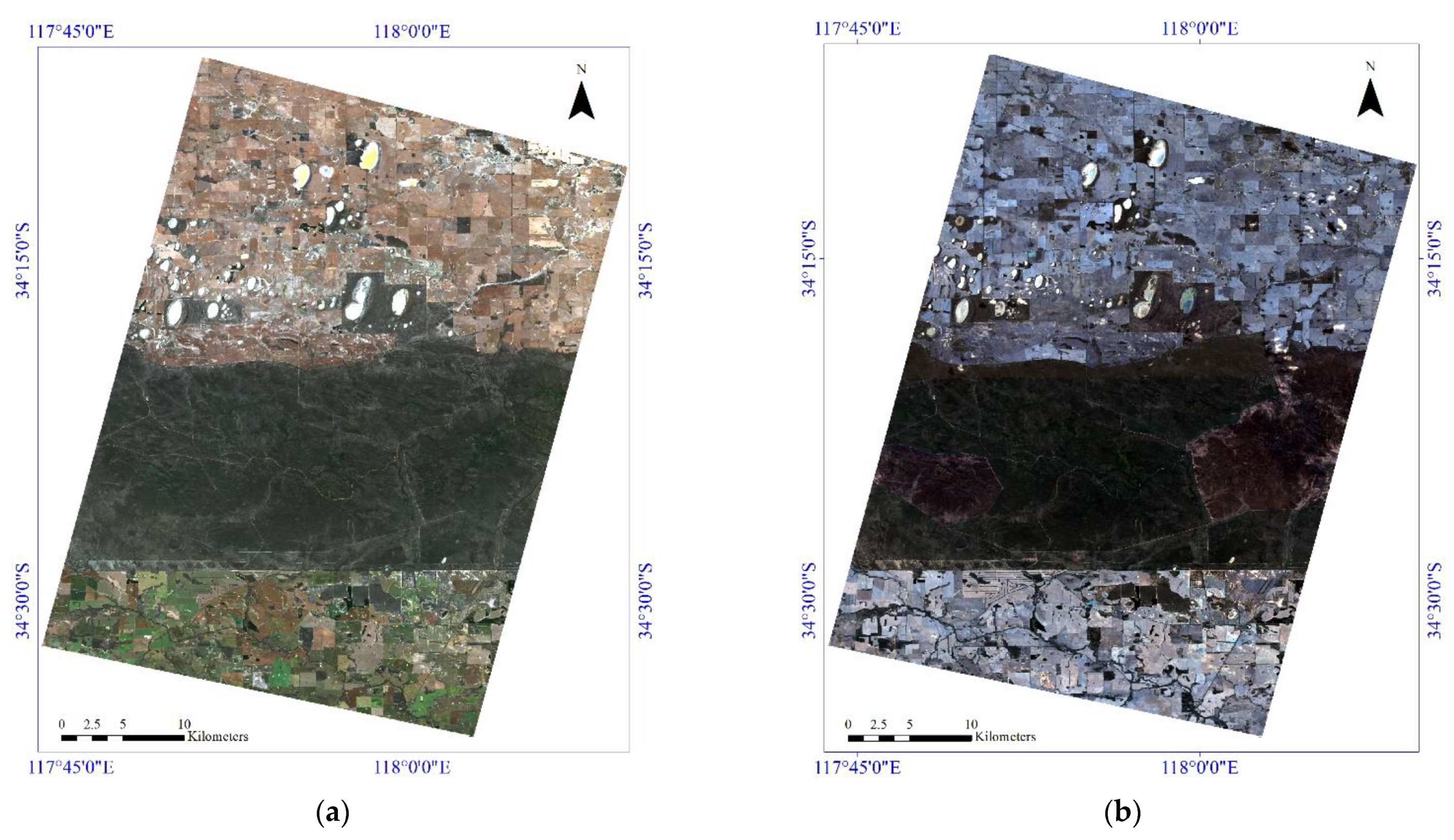
3.1. Study Area
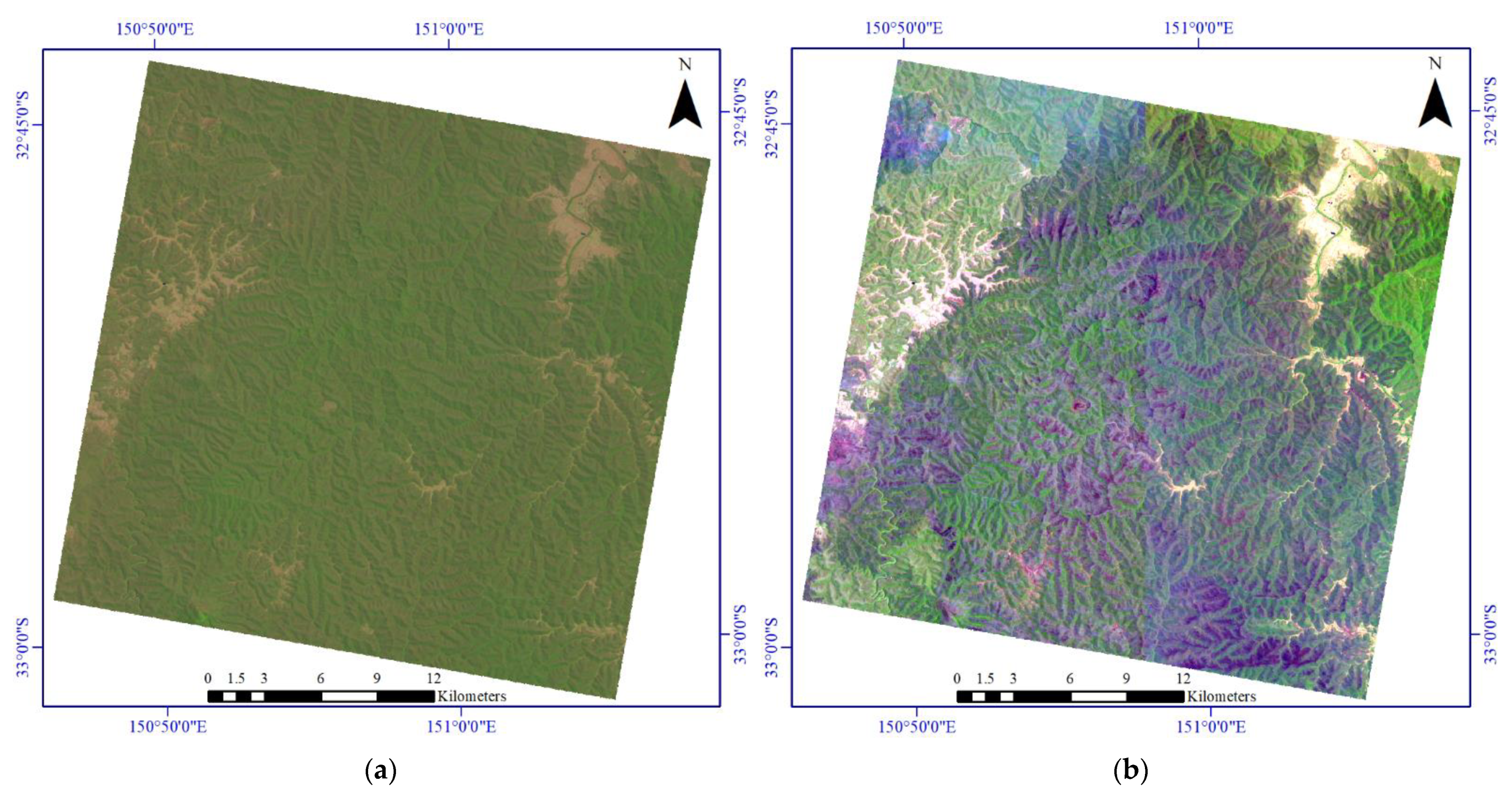
3.2. Sentinel-2 Images
3.3. PRISMA Images
4. Experiments and Results
4.1. Parameter Setting
4.2. Results
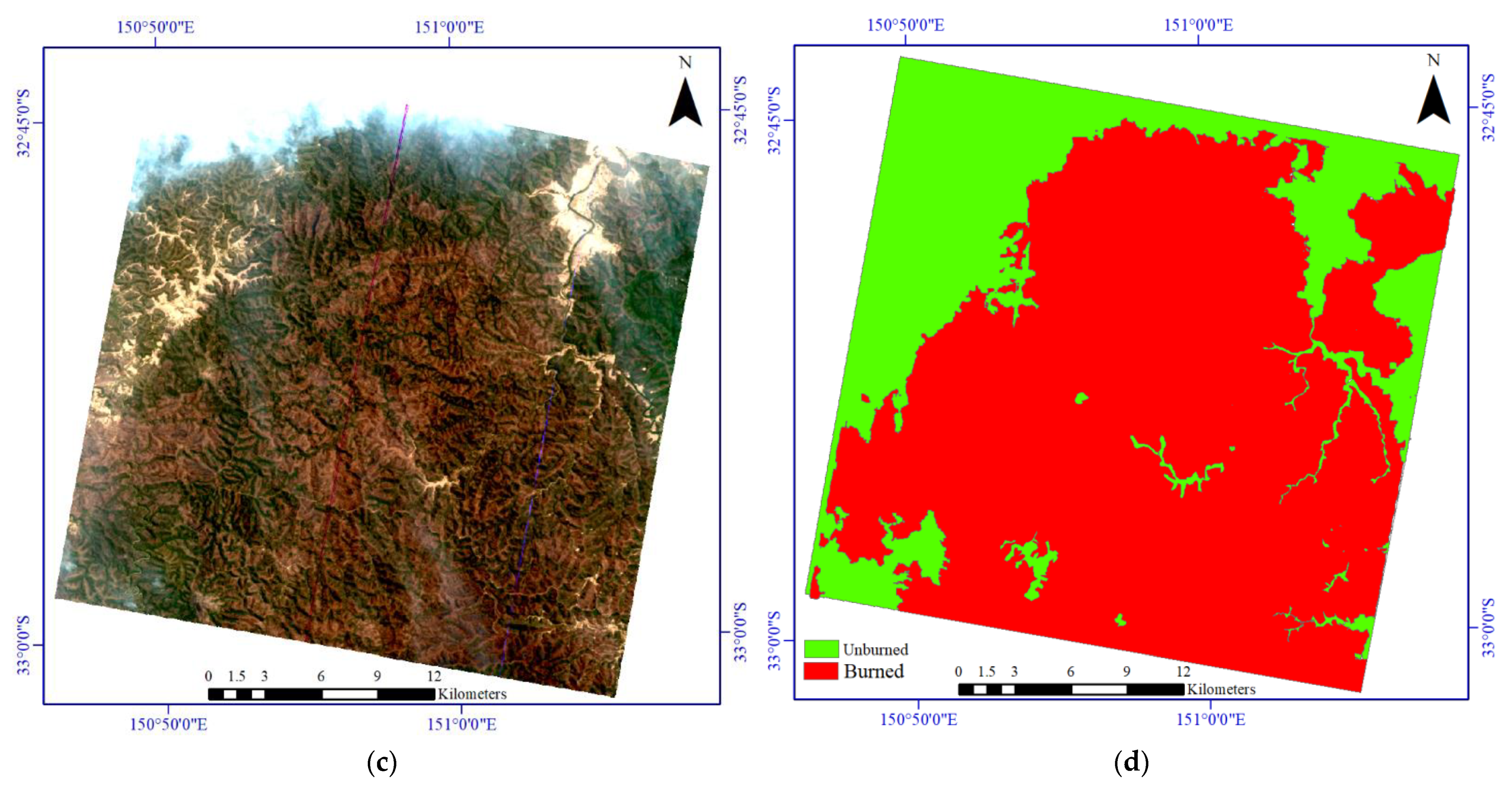
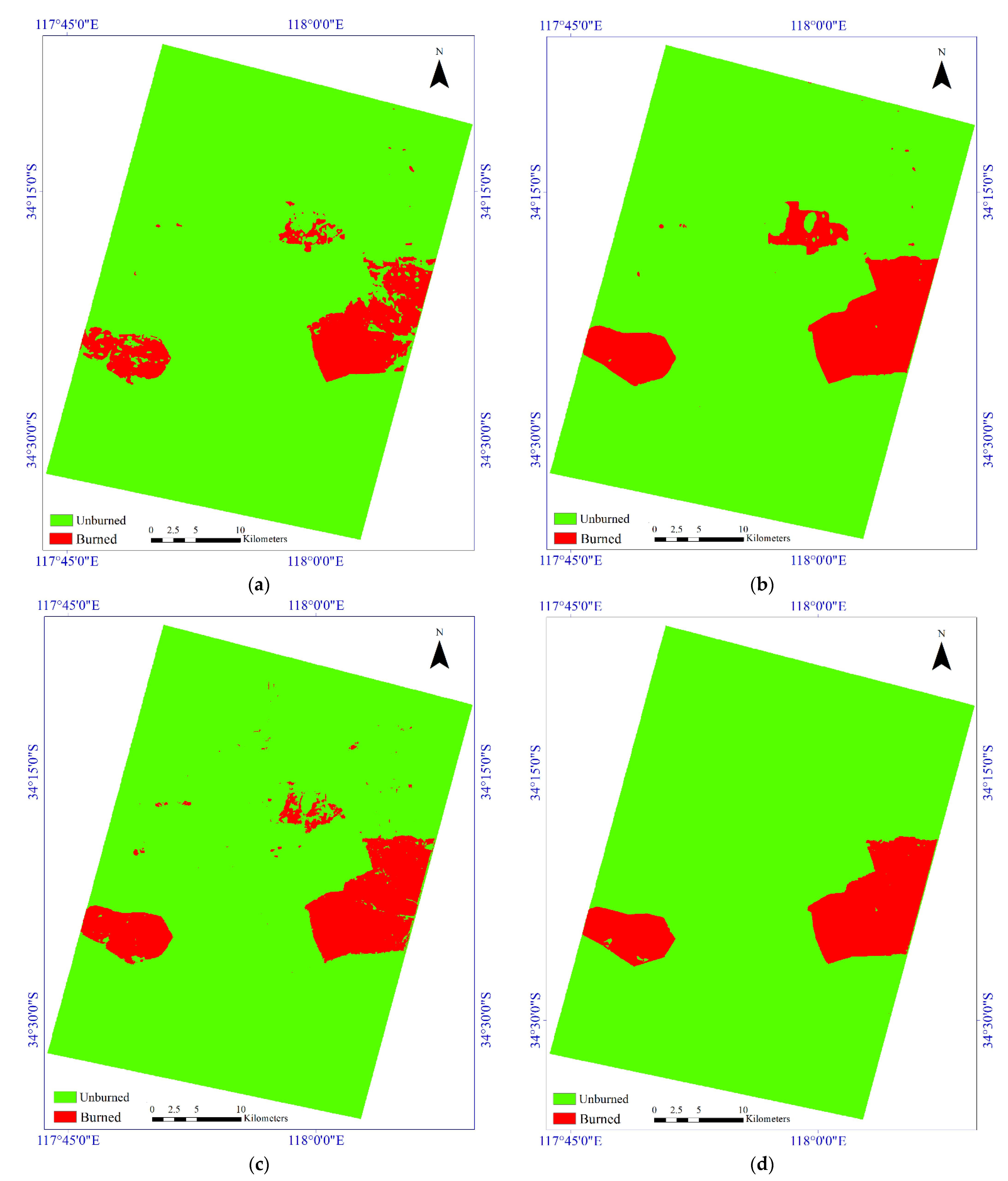
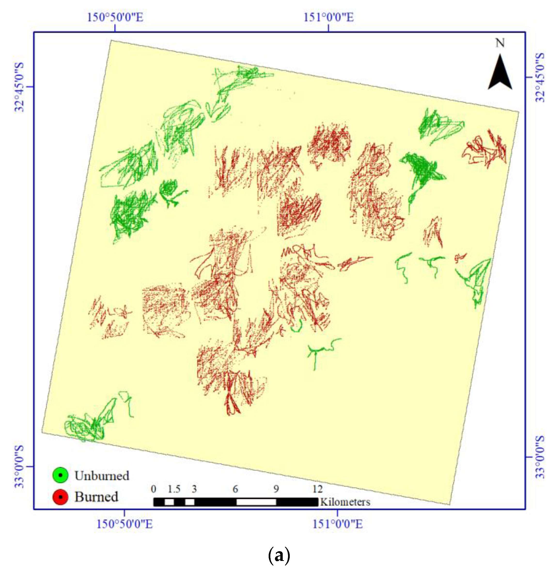
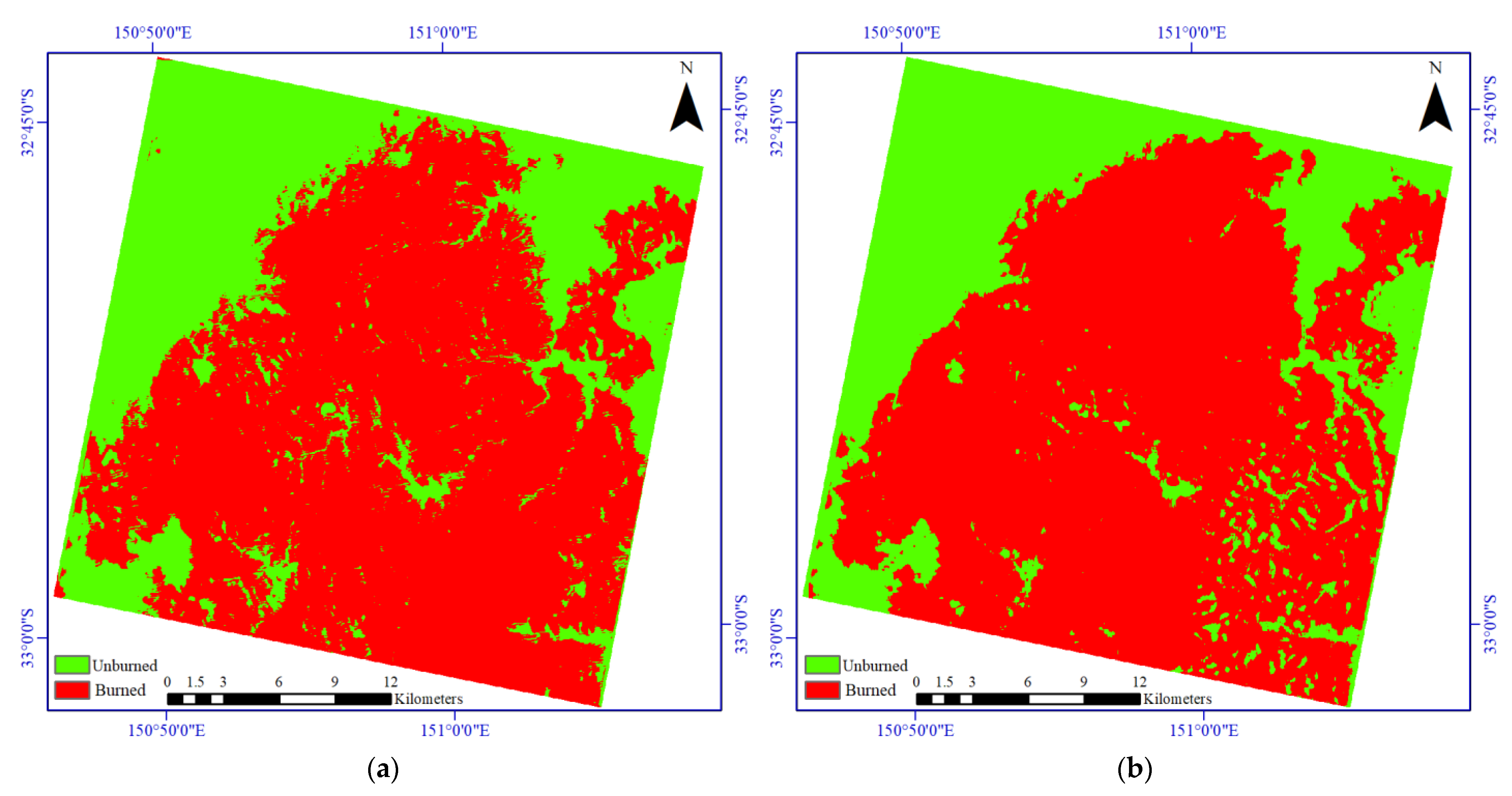
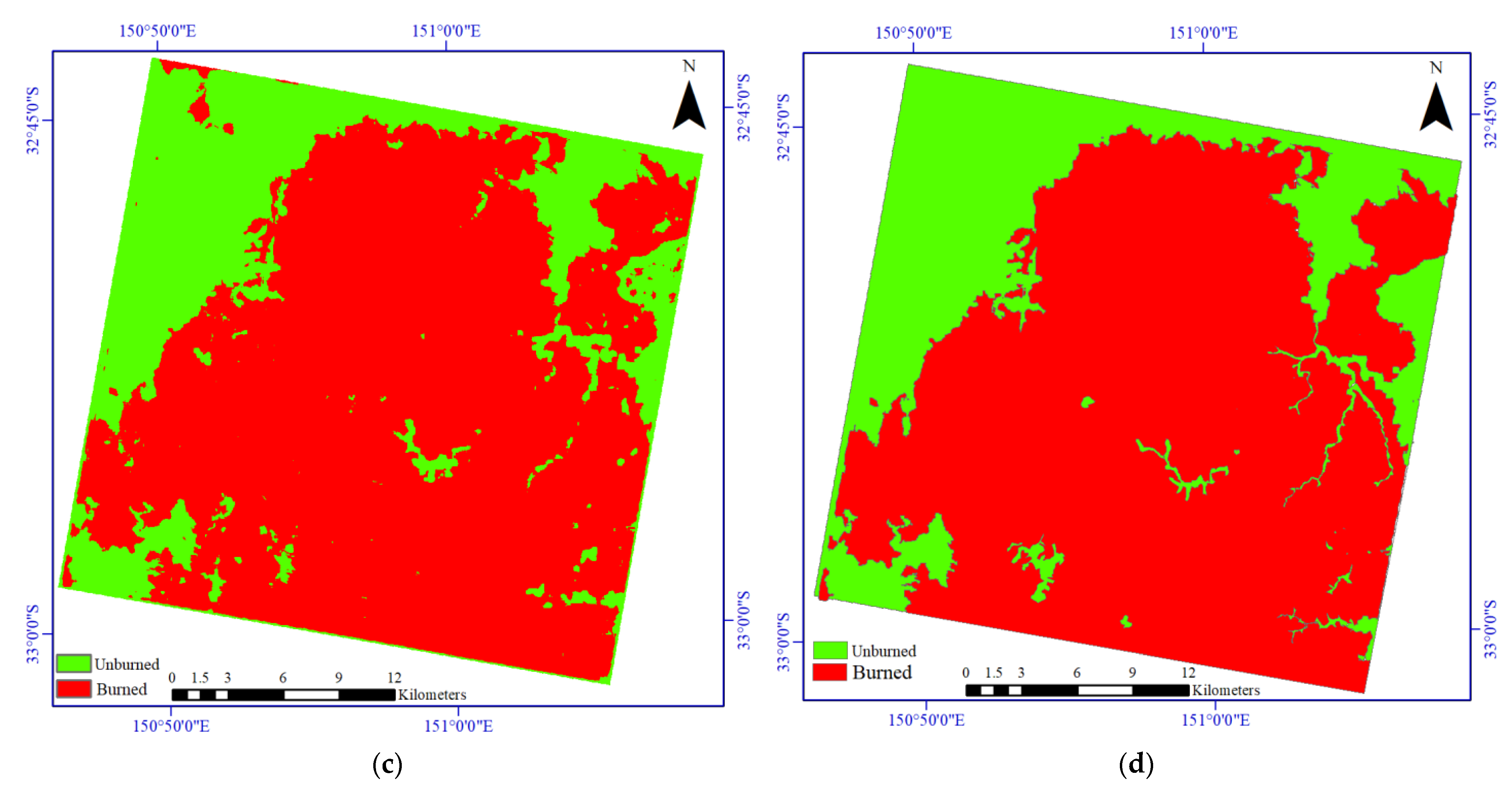
4.2.1. First Study Area
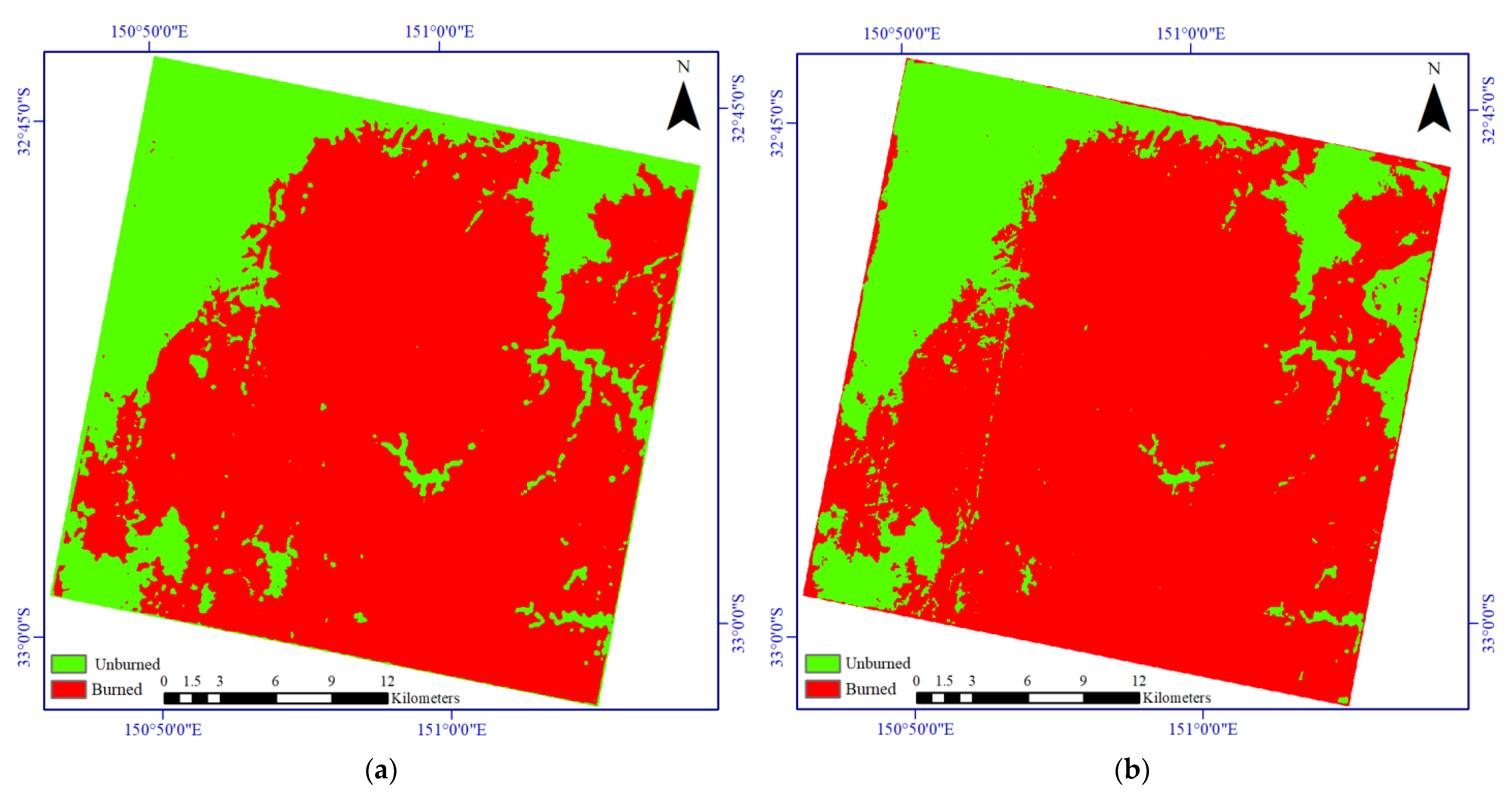
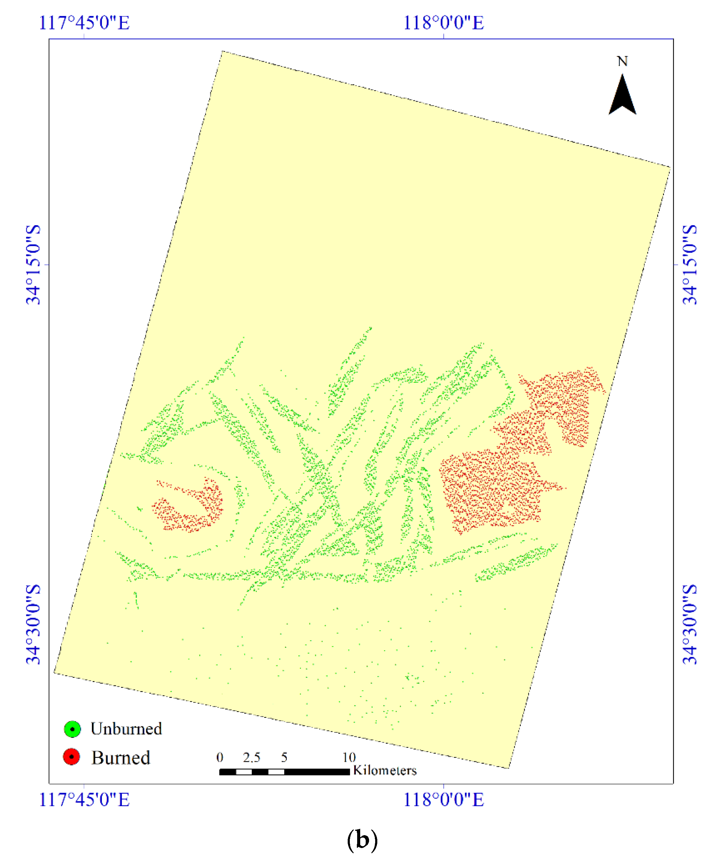
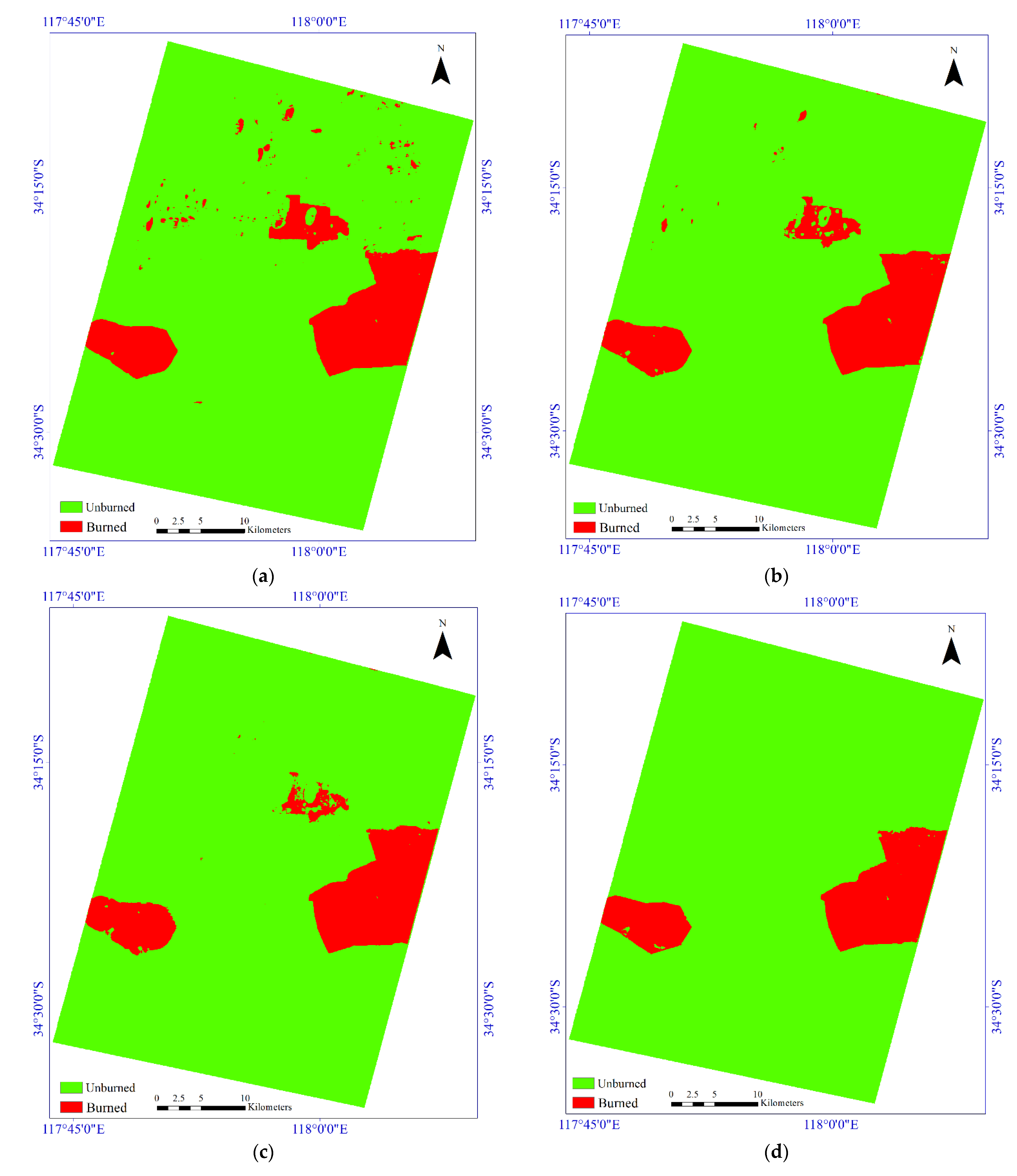
4.2.2. Second Study Area
5. Discussion
6. Conclusions
Author Contributions
Funding
Institutional Review Board Statement
Informed Consent Statement
Data Availability Statement
Acknowledgments
Conflicts of Interest
References
- Llorens, R.; Sobrino, J.A.; Fernández, C.; Fernández-Alonso, J.M.; Vega, J.A. A methodology to estimate forest fires burned areas and burn severity degrees using Sentinel-2 data. Application to the October 2017 fires in the Iberian Peninsula. Int. J. Appl. Earth Obs. Geoinf. 2021, 95, 102243. [Google Scholar] [CrossRef]
- Nohrstedt, D.; Mazzoleni, M.; Parker, C.F.; Di Baldassarre, G. Exposure to natural hazard events unassociated with policy change for improved disaster risk reduction. Nat. Commun. 2021, 12, 193. [Google Scholar] [CrossRef]
- Roy, D.P.; Li, Z.; Giglio, L.; Boschetti, L.; Huang, H. Spectral and diurnal temporal suitability of GOES Advanced Baseline Imager (ABI) reflectance for burned area mapping. Int. J. Appl. Earth Obs. Geoinf. 2021, 96, 102271. [Google Scholar] [CrossRef]
- de Luca, G.; Silva, J.M.; Modica, G. A workflow based on Sentinel-1 SAR data and open-source algorithms for unsupervised burned area detection in Mediterranean ecosystems. GIScience Remote Sens. 2021, 58, 516–541. [Google Scholar] [CrossRef]
- Duane, A.; Castellnou, M.; Brotons, L. Towards a comprehensive look at global drivers of novel extreme wildfire events. Clim. Chang. 2021, 165, 43. [Google Scholar] [CrossRef]
- Palaiologou, P.; Kalabokidis, K.; Troumbis, A.; Day, M.A.; Nielsen-Pincus, M.; Ager, A.A. Socio-Ecological Perceptions of Wildfire Management and Effects in Greece. Fire 2021, 4, 18. [Google Scholar] [CrossRef]
- Serra-Burriel, F.; Delicado, P.; Prata, A.T.; Cucchietti, F.M. Estimating heterogeneous wildfire effects using synthetic controls and satellite remote sensing. Remote Sens. Environ. 2021, 265, 112649. [Google Scholar] [CrossRef]
- Chowdhury, S.; Zhu, K.; Zhang, Y. Mitigating Greenhouse Gas Emissions Through Generative Adversarial Networks Based Wildfire Prediction. arXiv 2021, arXiv:2108.08952. [Google Scholar]
- Haque, M.K.; Azad, M.A.K.; Hossain, M.Y.; Ahmed, T.; Uddin, M.; Hossain, M.M. Wildfire in Australia during 2019–2020, Its Impact on Health, Biodiversity and Environment with Some Proposals for Risk Management: A Review. J. Environ. Prot. 2021, 12, 391–414. [Google Scholar] [CrossRef]
- Seydi, S.T.; Akhoondzadeh, M.; Amani, M.; Mahdavi, S. Wildfire damage assessment over Australia using sentinel-2 imagery and MODIS land cover product within the google earth engine cloud platform. Remote Sens. 2021, 13, 220. [Google Scholar] [CrossRef]
- Pandey, P.C.; Koutsias, N.; Petropoulos, G.P.; Srivastava, P.K.; Ben Dor, E. Land use/land cover in view of earth observation: Data sources, input dimensions, and classifiers—A review of the state of the art. Geocarto Int. 2021, 36, 957–988. [Google Scholar] [CrossRef]
- Seydi, S.T.; Hasanlou, M.; Amani, M.; Huang, W. Oil Spill Detection Based on Multi-Scale Multi-Dimensional Residual CNN for Optical Remote Sensing Imagery. IEEE J. Sel. Top. Appl. Earth Obs. Remote Sens. 2021, 14, 10941–10952. [Google Scholar] [CrossRef]
- Masek, J.G.; Wulder, M.A.; Markham, B.; McCorkel, J.; Crawford, C.J.; Storey, J.; Jenstrom, D.T. Landsat 9: Empowering open science and applications through continuity. Remote Sens. Environ. 2020, 248, 111968. [Google Scholar] [CrossRef]
- Vangi, E.; D’Amico, G.; Francini, S.; Giannetti, F.; Lasserre, B.; Marchetti, M.; Chirici, G. The new hyperspectral satellite PRISMA: Imagery for forest types discrimination. Sensors 2021, 21, 1182. [Google Scholar] [CrossRef]
- Wambugu, N.; Chen, Y.; Xiao, Z.; Wei, M.; Bello, S.A.; Junior, J.M.; Li, J. A hybrid deep convolutional neural network for accurate land cover classification. Int. J. Appl. Earth Obs. Geoinf. 2021, 103, 102515. [Google Scholar] [CrossRef]
- Xu, L.; Li, J.; Brenning, A. A comparative study of different classification techniques for marine oil spill identification using RADARSAT-1 imagery. Remote Sens. Environ. 2014, 141, 14–23. [Google Scholar] [CrossRef]
- Gu, Y.; Liu, T.; Gao, G.; Ren, G.; Ma, Y.; Chanussot, J.; Jia, X. Multimodal hyperspectral remote sensing: An overview and perspective. Sci. China Inf. Sci. 2021, 64, 1–24. [Google Scholar] [CrossRef]
- Hong, D.; Chanussot, J.; Zhu, X.X. An Overview of Multimodal Remote Sensing Data Fusion: From Image to Feature, from Shallow to Deep. In Proceedings of the 2021 IEEE International Geoscience and Remote Sensing Symposium IGARSS, Brussels, Belgium, 11–16 July 2021; pp. 1245–1248. [Google Scholar]
- Mardian, J.; Berg, A.; Daneshfar, B. Evaluating the temporal accuracy of grassland to cropland change detection using multitemporal image analysis. Remote Sens. Environ. 2021, 255, 112292. [Google Scholar] [CrossRef]
- Sun, Y.; Lei, L.; Li, X.; Sun, H.; Kuang, G. Nonlocal patch similarity based heterogeneous remote sensing change detection. Pattern Recognit. 2021, 109, 107598. [Google Scholar] [CrossRef]
- ElGharbawi, T.; Zarzoura, F. Damage detection using SAR coherence statistical analysis, application to Beirut, Lebanon. ISPRS J. Photogramm. Remote Sens. 2021, 173, 1–9. [Google Scholar] [CrossRef]
- Hashemi-Beni, L.; Gebrehiwot, A.A. Flood extent mapping: An integrated method using deep learning and region growing using UAV optical data. IEEE J. Sel. Top. Appl. Earth Obs. Remote Sens. 2021, 14, 2127–2135. [Google Scholar] [CrossRef]
- Liu, S.; Chi, M.; Zou, Y.; Samat, A.; Benediktsson, J.A.; Plaza, A. Oil spill detection via multitemporal optical remote sensing images: A change detection perspective. IEEE Geosci. Remote Sens. Lett. 2017, 14, 324–328. [Google Scholar] [CrossRef]
- Moya, L.; Geiß, C.; Hashimoto, M.; Mas, E.; Koshimura, S.; Strunz, G. Disaster Intensity-Based Selection of Training Samples for Remote Sensing Building Damage Classification. IEEE Trans. Geosci. Remote Sens. 2021, 59, 8288–8304. [Google Scholar] [CrossRef]
- Zheng, Z.; Zhong, Y.; Wang, J.; Ma, A.; Zhang, L. Building damage assessment for rapid disaster response with a deep object-based semantic change detection framework: From natural disasters to man-made disasters. Remote Sens. Environ. 2021, 265, 112636. [Google Scholar] [CrossRef]
- Hu, X.; Ban, Y.; Nascetti, A. Uni-Temporal Multispectral Imagery for Burned Area Mapping with Deep Learning. Remote Sens. 2021, 13, 1509. [Google Scholar] [CrossRef]
- Muñoz, D.F.; Muñoz, P.; Moftakhari, H.; Moradkhani, H. From local to regional compound flood mapping with deep learning and data fusion techniques. Sci. Total Environ. 2021, 782, 146927. [Google Scholar] [CrossRef]
- Zhang, Q.; Ge, L.; Zhang, R.; Metternicht, G.I.; Du, Z.; Kuang, J.; Xu, M. Deep-learning-based burned area mapping using the synergy of Sentinel-1&2 data. Remote Sens. Environ. 2021, 264, 112575. [Google Scholar]
- Chiang, S.-H.; Ulloa, N.I. Mapping and Tracking Forest Burnt Areas in the Indio Maiz Biological Reserve Using Sentinel-3 SLSTR and VIIRS-DNB Imagery. Sensors 2019, 19, 5423. [Google Scholar] [CrossRef] [Green Version]
- Lizundia-Loiola, J.; Franquesa, M.; Boettcher, M.; Kirches, G.; Pettinari, M.L.; Chuvieco, E. Implementation of the Burned Area Component of the Copernicus Climate Change Service: From MODIS to OLCI Data. Remote Sens. 2021, 13, 4295. [Google Scholar] [CrossRef]
- Pinto, M.M.; Trigo, R.M.; Trigo, I.F.; DaCamara, C.C. A Practical Method for High-Resolution Burned Area Monitoring Using Sentinel-2 and VIIRS. Remote Sens. 2021, 13, 1608. [Google Scholar] [CrossRef]
- Donezar, U.; De Blas, T.; Larrañaga, A.; Ros, F.; Albizua, L.; Steel, A.; Broglia, M. Applicability of the multitemporal coherence approach to sentinel-1 for the detection and delineation of burnt areas in the context of the copernicus emergency management service. Remote Sens. 2019, 11, 2607. [Google Scholar] [CrossRef] [Green Version]
- Xulu, S.; Mbatha, N.; Peerbhay, K. Burned Area Mapping over the Southern Cape Forestry Region, South Africa Using Sentinel Data within GEE Cloud Platform. ISPRS Int. J. Geo-Inf. 2021, 10, 511. [Google Scholar] [CrossRef]
- Liu, S.; Zheng, Y.; Dalponte, M.; Tong, X. A novel fire index-based burned area change detection approach using Landsat-8 OLI data. Eur. J. Remote Sens. 2020, 53, 104–112. [Google Scholar] [CrossRef] [Green Version]
- Nolde, M.; Plank, S.; Riedlinger, T. An Adaptive and Extensible System for Satellite-Based, Large Scale Burnt Area Monitoring in Near-Real Time. Remote Sens. 2020, 12, 2162. [Google Scholar] [CrossRef]
- Knopp, L.; Wieland, M.; Rättich, M.; Martinis, S. A deep learning approach for burned area segmentation with Sentinel-2 data. Remote Sens. 2020, 12, 2422. [Google Scholar] [CrossRef]
- de Bem, P.P.; de Carvalho Júnior, O.A.; de Carvalho, O.L.F.; Gomes, R.A.T.; Fontes Guimarães, R. Performance analysis of deep convolutional autoencoders with different patch sizes for change detection from burnt areas. Remote Sens. 2020, 12, 2576. [Google Scholar] [CrossRef]
- Ban, Y.; Zhang, P.; Nascetti, A.; Bevington, A.R.; Wulder, M.A. Near real-time wildfire progression monitoring with Sentinel-1 SAR time series and deep learning. Sci. Rep. 2020, 10, 1322. [Google Scholar] [CrossRef] [Green Version]
- Zhang, P.; Ban, Y.; Nascetti, A. Learning U-Net without forgetting for near real-time wildfire monitoring by the fusion of SAR and optical time series. Remote Sens. Environ. 2021, 261, 112467. [Google Scholar] [CrossRef]
- Farasin, A.; Colomba, L.; Garza, P. Double-step u-net: A deep learning-based approach for the estimation of wildfire damage severity through sentinel-2 satellite data. Appl. Sci. 2020, 10, 4332. [Google Scholar] [CrossRef]
- Lestari, A.I.; Rizkinia, M.; Sudiana, D. Evaluation of Combining Optical and SAR Imagery for Burned Area Mapping using Machine Learning. In Proceedings of the 2021 IEEE 11th Annual Computing and Communication Workshop and Conference (CCWC), Virtual, 27–30 January 2021; pp. 0052–0059. [Google Scholar]
- Belenguer-Plomer, M.A.; Tanase, M.A.; Chuvieco, E.; Bovolo, F. CNN-based burned area mapping using radar and optical data. Remote Sens. Environ. 2021, 260, 112468. [Google Scholar] [CrossRef]
- Proy, C.; Tanre, D.; Deschamps, P. Evaluation of topographic effects in remotely sensed data. Remote Sens. Environ. 1989, 30, 21–32. [Google Scholar] [CrossRef]
- Hao, D.; Wen, J.; Xiao, Q.; Wu, S.; Lin, X.; You, D.; Tang, Y. Modeling anisotropic reflectance over composite sloping terrain. IEEE Trans. Geosci. Remote Sens. 2018, 56, 3903–3923. [Google Scholar] [CrossRef]
- Pouyap, M.; Bitjoka, L.; Mfoumou, E.; Toko, D. Improved Bearing Fault Diagnosis by Feature Extraction Based on GLCM, Fusion of Selection Methods, and Multiclass-Naïve Bayes Classification. J. Signal Inf. Process. 2021, 12, 71–85. [Google Scholar]
- Raja, G.; Dev, K.; Philips, N.D.; Suhaib, S.M.; Deepakraj, M.; Ramasamy, R.K. DA-WDGN: Drone-Assisted Weed Detection using GLCM-M features and NDIRT indices. In Proceedings of the IEEE INFOCOM 2021-IEEE Conference on Computer Communications Workshops (INFOCOM WKSHPS), Vancouver, BC, Canada, 10–13 May 2021; pp. 1–6. [Google Scholar]
- Liu, W.; Wang, C.; Chen, S.; Bian, X.; Lai, B.; Shen, X.; Cheng, M.; Lai, S.-H.; Weng, D.; Li, J. Y-Net: Learning Domain Robust Feature Representation for Ground Camera Image and Large-scale Image-based Point Cloud Registration. Inf. Sci. 2021, 581, 655–677. [Google Scholar] [CrossRef]
- Yu, Y.; Wang, J.; Qiang, H.; Jiang, M.; Tang, E.; Yu, C.; Zhang, Y.; Li, J. Sparse anchoring guided high-resolution capsule network for geospatial object detection from remote sensing imagery. Int. J. Appl. Earth Obs. Geoinf. 2021, 104, 102548. [Google Scholar] [CrossRef]
- Chen, Y.; Jiang, H.; Li, C.; Jia, X.; Ghamisi, P. Deep feature extraction and classification of hyperspectral images based on convolutional neural networks. IEEE Trans. Geosci. Remote Sens. 2016, 54, 6232–6251. [Google Scholar] [CrossRef] [Green Version]
- Li, Y.; Cui, P.; Ye, C.; Junior, J.M.; Zhang, Z.; Guo, J.; Li, J. Accurate Prediction of Earthquake-Induced Landslides Based on Deep Learning Considering Landslide Source Area. Remote Sens. 2021, 13, 3436. [Google Scholar] [CrossRef]
- Seydi, S.T.; Hasanlou, M. A New Structure for Binary and Multiple Hyperspectral Change Detection Based on Spectral Unmixing and Convolutional Neural Network. Measurement 2021, 186, 110137. [Google Scholar] [CrossRef]
- Roy, S.K.; Kar, P.; Hong, D.; Wu, X.; Plaza, A.; Chanussot, J. Revisiting Deep Hyperspectral Feature Extraction Networks via Gradient Centralized Convolution. IEEE Trans. Geosci. Remote Sens. 2021. [Google Scholar] [CrossRef]
- Yu, Q.; Wang, S.; He, H.; Yang, K.; Ma, L.; Li, J. Reconstructing GRACE-like TWS anomalies for the Canadian landmass using deep learning and land surface model. Int. J. Appl. Earth Obs. Geoinf. 2021, 102, 102404. [Google Scholar] [CrossRef]
- Wu, C.; Zhang, F.; Xia, J.; Xu, Y.; Li, G.; Xie, J.; Du, Z.; Liu, R. Building Damage Detection Using U-Net with Attention Mechanism from Pre-and Post-Disaster Remote Sensing Datasets. Remote Sens. 2021, 13, 905. [Google Scholar] [CrossRef]
- Dhaka, V.S.; Meena, S.V.; Rani, G.; Sinwar, D.; Ijaz, M.F.; Woźniak, M. A survey of deep convolutional neural networks applied for prediction of plant leaf diseases. Sensors 2021, 21, 4749. [Google Scholar] [CrossRef] [PubMed]
- Li, Z.; Liu, F.; Yang, W.; Peng, S.; Zhou, J. A survey of convolutional neural networks: Analysis, applications, and prospects. IEEE Trans. Neural Netw. Learn. Syst. 2021, 1–21. [Google Scholar] [CrossRef] [PubMed]
- Rawat, W.; Wang, Z. Deep convolutional neural networks for image classification: A comprehensive review. Neural Comput. 2017, 29, 2352–2449. [Google Scholar] [CrossRef]
- Goodfellow, I.; Bengio, Y.; Courville, A. Deep Learning; MIT Press: Cambridge, MA, USA, 2016. [Google Scholar]
- Lu, L.; Wang, X.; Carneiro, G.; Yang, L. Deep Learning and Convolutional Neural Networks for Medical Imaging and Clinical Informatics; Springer: Cham, Switzerland, 2019. [Google Scholar]
- DeLancey, E.R.; Simms, J.F.; Mahdianpari, M.; Brisco, B.; Mahoney, C.; Kariyeva, J. Comparing deep learning and shallow learning for large-scale wetland classification in Alberta, Canada. Remote Sens. 2020, 12, 2. [Google Scholar] [CrossRef] [Green Version]
- Seydi, S.; Rastiveis, H. A Deep Learning Framework for Roads Network Damage Assessment Using Post-Earthquake Lidar Data. Int. Arch. Photogramm. Remote Sens. Spat. Inf. Sci. 2019. [Google Scholar] [CrossRef] [Green Version]
- Yu, C.; Han, R.; Song, M.; Liu, C.; Chang, C.-I. A simplified 2D-3D CNN architecture for hyperspectral image classification based on spatial–spectral fusion. IEEE J. Sel. Top. Appl. Earth Obs. Remote Sens. 2020, 13, 2485–2501. [Google Scholar] [CrossRef]
- Nogueira, K.; Chanussot, J.; Dalla Mura, M.; Dos Santos, J.A. An introduction to deep morphological networks. IEEE Access 2021, 9, 114308–114324. [Google Scholar] [CrossRef]
- Limonova, E.E.; Alfonso, D.M.; Nikolaev, D.P.; Arlazarov, V.V. Bipolar Morphological Neural Networks: Gate-Efficient Architecture for Computer Vision. IEEE Access 2021, 9, 97569–97581. [Google Scholar] [CrossRef]
- Shen, Y.; Zhong, X.; Shih, F.Y. Deep morphological neural networks. arXiv Prepr. 2019, arXiv:1909.01532. [Google Scholar]
- Franchi, G.; Fehri, A.; Yao, A. Deep morphological networks. Pattern Recognit. 2020, 102, 107246. [Google Scholar] [CrossRef]
- Islam, M.A.; Murray, B.; Buck, A.; Anderson, D.T.; Scott, G.J.; Popescu, M.; Keller, J. Extending the morphological hit-or-miss transform to deep neural networks. IEEE Trans. Neural Netw. Learn. Syst. 2020, 32, 4826–4838. [Google Scholar] [CrossRef] [PubMed]
- Klemen, M.; Krsnik, L.; Robnik-Šikonja, M. Enhancing deep neural networks with morphological information. arXiv Prepr. 2020, arXiv:2011.12432. [Google Scholar]
- Mondal, R. Morphological Network: Network with Morphological Neurons; Indian Statistical Institute: Kolkata, India, 2021. [Google Scholar]
- Salehi, S.S.M.; Erdogmus, D.; Gholipour, A. Tversky loss function for image segmentation using 3D fully convolutional deep networks. In Proceedings of the International Workshop on Machine Learning in Medical Imaging, Quebec City, QC, Canada, 10 September 2017; pp. 379–387. [Google Scholar]
- Zhan, Y.; Fu, K.; Yan, M.; Sun, X.; Wang, H.; Qiu, X. Change detection based on deep siamese convolutional network for optical aerial images. IEEE Geosci. Remote Sens. Lett. 2017, 14, 1845–1849. [Google Scholar] [CrossRef]
- Arabi, M.E.A.; Karoui, M.S.; Djerriri, K. Optical remote sensing change detection through deep siamese network. In Proceedings of the IGARSS 2018—2018 IEEE International Geoscience and Remote Sensing Symposium, Valencia, Spain, 22–27 July 2018; pp. 5041–5044. [Google Scholar]
- Yang, L.; Chen, Y.; Song, S.; Li, F.; Huang, G. Deep Siamese networks based change detection with remote sensing images. Remote Sens. 2021, 13, 3394. [Google Scholar] [CrossRef]
- Guarini, R.; Loizzo, R.; Facchinetti, C.; Longo, F.; Ponticelli, B.; Faraci, M.; Dami, M.; Cosi, M.; Amoruso, L.; De Pasquale, V. PRISMA Hyperspectral Mission Products. In Proceedings of the IGARSS 2018—2018 IEEE International Geoscience and Remote Sensing Symposium, Valencia, Spain, 22–27 July 2018; pp. 179–182. [Google Scholar]
- Loizzo, R.; Guarini, R.; Longo, F.; Scopa, T.; Formaro, R.; Facchinetti, C.; Varacalli, G. PRISMA: The Italian Hyperspectral Mission. In Proceedings of the IGARSS 2018—2018 IEEE International Geoscience and Remote Sensing Symposium, Valencia, Spain, 22–27 July 2018; pp. 175–178. [Google Scholar]
- He, K.; Zhang, X.; Ren, S.; Sun, J. Delving deep into rectifiers: Surpassing human-level performance on imagenet classification. In Proceedings of the IEEE International Conference on Computer Vision, Santiago, Chile, 7–13 December 2015; pp. 1026–1034. [Google Scholar]
- Grivei, A.-C.; Văduva, C.; Datcu, M. Assessment of Burned Area Mapping Methods for Smoke Covered Sentinel-2 Data. In Proceedings of the 2020 13th International Conference on Communications (COMM), Bucharest, Romania, 18–20 June 2020; pp. 189–192. [Google Scholar]
- Barboza Castillo, E.; Turpo Cayo, E.Y.; de Almeida, C.M.; Salas López, R.; Rojas Briceño, N.B.; Silva López, J.O.; Barrena Gurbillón, M.Á.; Oliva, M.; Espinoza-Villar, R. Monitoring wildfires in the northeastern peruvian amazon using landsat-8 and sentinel-2 imagery in the GEE platform. ISPRS Int. J. Geo-Inf. 2020, 9, 564. [Google Scholar] [CrossRef]
- Syifa, M.; Panahi, M.; Lee, C.-W. Mapping of post-wildfire burned area using a hybrid algorithm and satellite data: The case of the camp fire wildfire in California, USA. Remote Sens. 2020, 12, 623. [Google Scholar] [CrossRef] [Green Version]
- Quintano, C.; Fernández-Manso, A.; Fernández-Manso, O. Combination of Landsat and Sentinel-2 MSI data for initial assessing of burn severity. Int. J. Appl. Earth Obs. Geoinf. 2018, 64, 221–225. [Google Scholar] [CrossRef]
- Ngadze, F.; Mpakairi, K.S.; Kavhu, B.; Ndaimani, H.; Maremba, M.S. Exploring the utility of Sentinel-2 MSI and Landsat 8 OLI in burned area mapping for a heterogenous savannah landscape. PLoS ONE 2020, 15, e0232962. [Google Scholar] [CrossRef]
- Roy, D.P.; Huang, H.; Boschetti, L.; Giglio, L.; Yan, L.; Zhang, H.H.; Li, Z. Landsat-8 and Sentinel-2 burned area mapping-A combined sensor multi-temporal change detection approach. Remote Sens. Environ. 2019, 231, 111254. [Google Scholar] [CrossRef]
- Lima, T.A.; Beuchle, R.; Langner, A.; Grecchi, R.C.; Griess, V.C.; Achard, F. Comparing Sentinel-2 MSI and Landsat 8 OLI imagery for monitoring selective logging in the Brazilian Amazon. Remote Sens. 2019, 11, 961. [Google Scholar] [CrossRef] [Green Version]


| Sensor | Properties | First Study Area | Second Study Area |
|---|---|---|---|
| Sentinel-2 | Spectral bands | 13 | 13 |
| Spatial resolution (m) | 10 | 10 | |
| Resampled spatial resolution (m) | 30 | 30 | |
| Data size (pixel) | 1168 × 1168 | 1159 × 1853 | |
| Pre-event acquired date | December 2019 | October 2019 | |
| Post-event acquired date | November 2020 | January 2020 | |
| PRISMA | Spectral bands | 169 | 169 |
| Spatial resolution (m) | 30 | 30 | |
| Data size (pixel) | 1168 × 1168 | 1159 × 1853 | |
| Post-event acquired date | December 2019 | January 2020 |
| Case Study | Number of Pixels in the Study Area | Class | Number of Samples | Training | Validation | Testing |
|---|---|---|---|---|---|---|
| First study area | 989,764 | Unburned | 15,318 | 9803 | 2450 | 3065 |
| Burned | 21,387 | 13,687 | 3421 | 4459 | ||
| Second study area | 1,955,898 | Unburned | 6590 | 4217 | 1054 | 1318 |
| Burned | 3206 | 2051 | 513 | 642 |
| Scenario | Pre-Event Dataset | Post-Event Dataset |
|---|---|---|
| S#1 | Sentinel-2 | Sentinel-2 |
| S#2 | Sentinel-2 | PRISMA |
| Method | Scenario | OA (%) | Recall (%) | F1-Score (%) | IOU | KC |
|---|---|---|---|---|---|---|
| Siamese network | S#1 | 87.94 | 87.10 | 91.34 | 0.740 | 0.716 |
| S#2 | 94.79 | 96.19 | 96.43 | 0.786 | 0.868 | |
| CNN method proposed by [42] | S#1 | 89.35 | 89.40 | 92.46 | 0.842 | 0.744 |
| S#2 | 94.35 | 97.13 | 96.17 | 0.851 | 0.853 | |
| DSMNN-Net | S#1 | 90.24 | 92.51 | 93.26 | 0.864 | 0.755 |
| S#2 | 97.46 | 97.99 | 98.25 | 0.901 | 0.936 |
| Method | Scenario | OA (%) | Recall (%) | F1-Score (%) | IOU | KC |
|---|---|---|---|---|---|---|
| Siamese network | S#1 | 97.32 | 78.90 | 85.03 | 0.739 | 0.835 |
| S#2 | 97.41 | 98.79 | 88.05 | 0.786 | 0.866 | |
| CNN method proposed by [42] | S#1 | 98.21 | 98.94 | 91.44 | 0.842 | 0.904 |
| S#2 | 98.35 | 97.75 | 91.94 | 0.851 | 0.910 | |
| DSMNN-Net | S#1 | 98.56 | 95.13 | 92.75 | 0.864 | 0.919 |
| S#2 | 98.95 | 98.90 | 94.80 | 0.901 | 0.942 |
| Reference | Accuracy | Method | Dataset |
|---|---|---|---|
| Grivei, et al. [77] | (F1-Score: 0.873) | Support vector machine algorithm and spectral indices, factor analysis | Sentinel-2 |
| Barboza Castillo, et al. [78] | 94.4 | Thresholding on the spectral index | Sentinel-2 |
| Syifa, et al. [79] | 92 | Support vector machine and imperialist competitive algorithm | Sentinel-2 |
| Quintano, et al. [80] | 84 | Spectral index and thresholding | Combination of Landsat-8 and Sentinel-2 |
| Ngadze, et al. [81] | 92 | Random forest | Sentinel-2 |
| Roy, et al. [82] | 92 | Random forest change regression, and a region growing manner | Combination of Landsat-8 and Sentinel-2 |
| Lima, et al. [83] | 96 | Thresholding on the spectral index | Sentinel-2 |
| Seydi, Akhoondzadeh, Amani and Mahdavi [10] | 91 | Spectral and spatial features and random forest | Sentinel-2 |
| DSMNN-Net | 98 | Deep-learning based | Sentinel-2 |
Publisher’s Note: MDPI stays neutral with regard to jurisdictional claims in published maps and institutional affiliations. |
© 2021 by the authors. Licensee MDPI, Basel, Switzerland. This article is an open access article distributed under the terms and conditions of the Creative Commons Attribution (CC BY) license (https://creativecommons.org/licenses/by/4.0/).
Share and Cite
Seydi, S.T.; Hasanlou, M.; Chanussot, J. DSMNN-Net: A Deep Siamese Morphological Neural Network Model for Burned Area Mapping Using Multispectral Sentinel-2 and Hyperspectral PRISMA Images. Remote Sens. 2021, 13, 5138. https://doi.org/10.3390/rs13245138
Seydi ST, Hasanlou M, Chanussot J. DSMNN-Net: A Deep Siamese Morphological Neural Network Model for Burned Area Mapping Using Multispectral Sentinel-2 and Hyperspectral PRISMA Images. Remote Sensing. 2021; 13(24):5138. https://doi.org/10.3390/rs13245138
Chicago/Turabian StyleSeydi, Seyd Teymoor, Mahdi Hasanlou, and Jocelyn Chanussot. 2021. "DSMNN-Net: A Deep Siamese Morphological Neural Network Model for Burned Area Mapping Using Multispectral Sentinel-2 and Hyperspectral PRISMA Images" Remote Sensing 13, no. 24: 5138. https://doi.org/10.3390/rs13245138
APA StyleSeydi, S. T., Hasanlou, M., & Chanussot, J. (2021). DSMNN-Net: A Deep Siamese Morphological Neural Network Model for Burned Area Mapping Using Multispectral Sentinel-2 and Hyperspectral PRISMA Images. Remote Sensing, 13(24), 5138. https://doi.org/10.3390/rs13245138