A Novel 4D Track-before-Detect Approach for Weak Targets Detection in Clutter Regions

Abstract

A 4D TBD approach is developed here for closely weak extended target tracking and overcoming heterogeneous clutter background and various clutter regions. The 4D measurements in this work are the points containing three positional information in spatial space and corresponding timestamp. The proposed method is mainly designed to address two issues. The first one is the dilemma between the weak target detection and difficult computation originating from the high dimensions of measurement. The second issue is the suppression of inhomogeneous background clutter and various clutter regions. The extension experiment using synthetic data showcases that no false alarm track would be built in the clutter regions, and the detection rate of close targets exceeds 94%. The experiments using real 3D radar also prove that the method works well in tracking closely maneuvering extended targets even if a clutter region exists.

1. Introduction

In this work, a 4D TBD approach method is developed to detect the weak tracks in 3D radar systems. The 4D information of measurement includes the 3D position and its timestamp. Two extensively existing issues greatly deteriorate the target tracking performance in the application of 3D radars. The first issue is the dilemma between the weak extended target detection and difficult computation originating from the high dimensions of measurement [1].

The targets in this work are assumed extended targets [2]. The PHD filter [3] and CPHD filter [4] have been developed for multiple extended target tracking. Compared with single point target tracking, measurement partition [5] should be added before using a PHD filter. Extensive computation will be necessary to associate all possible measurement partitions with potential tracks, especially where lots of targets or measurements exist [3]. In [6,7], raw hydrophone data of a bistatic architecture sonar are processed using a TBD strategy, where several consecutive scans (or frames) are jointly processed, relying on target kinematics or, simply, exploiting the physically admissible target transitions, jointly declaring the presence of a target [8]. The unthresholded data in [6,7,8] are far more than the normal measurements. Therefore, extended target tracking using a TBD method strategy is a computationally complex task. In the issue of weak trajectory detection, various TBD methods have been developed such as DP-TBD [9,10,11], PF-TBD [12,13,14,15,16], HT-TBD [2,17,18,19], and some optimization based TBD [20]. In 3D target tracking scenarios, the computation of the TBD methods [9,10,12,13,14,17,18,20] will sharply increase for a satisfying tracking performance. It is mainly because all possible high-dimensional solutions are exploited. The methods [2,19,21] are designed for 2D radars whose position information only contains the X axis and Y axis. Therefore, to solve the problem, the proposed 4D TBD consists of two stages. A 3D TBD in the first stage is designed to filter out the majority of clutter points, and multiple 2D TBD in the second stage is used to carefully detect the tracks with the reserved measurements. Therefore, the proposed method is efficient in dealing with high-dimensional measurements and maintains a remarkably good performance in tracking weak extended targets.

The proposed method here is designed to track the weak targets in uniform linear motion and slowly maneuvering targets, especially for aircraft, using air surveillance radar [22]. In our former work [13,19,21], tracking maneuvering targets [23] were divided into two stages, tracklet generation and tracklet association. In maneuvering target tracking cases, extended target tracklets can be extracted by the proposed method. In the tracklet association, the tracklets of the same target are associated to get the whole maneuvering trajectory. The tracklets are far fewer than the points, which decreases the computation of obtaining trajectory by associating points directly. Therefore, the maneuvering target tracking problem can be also addressed with fewer extra computations.

The second issue is the clutter region suppression [24]. The regions in the surveillance area can be quite different. For example, downtown areas usually generate far more false alarm points than villages. The nonhomogeneity of the surveillance region makes the tracking method very sensitive to false alarms and target miss-detection. In these scenarios, the clutter region suppression is significant in reducing false tracks and improving true target track life [25]. To address this issue, Spatio-temporal detection [26], a clutter map [27], and a prior knowledge-based method [25] have been developed to suppress the clutter region. In [25,28,29,30], clutter region suppression using a clutter map is applied as pre-processing before target tracking. In [25,28], the clutter regions are labeled and then the measurements or initial tracks in these regions are removed. In [29,30], the clutter densities of different regions are considered, and the clutter map is integrated with standard tracking methods. The points that originated from low clutter density regions are given a higher weight and are more likely to be associated with a track.

In the proposed method, rather than estimating point weight with a clutter map, a novel clutter map in each detection bin is integrated with the TBD method. The component of various clutter regions and background can be well canceled in track detection.

Not only the two issues mentioned above, but other issues, such as the ability to cope with multiple close tracks and the universality of the extended target and non-extended target, are also addressed in this work. The merits are validated by both simulation and real experiments of 3D radar.

This paper is organized as follows. Section 2 introduces the system and state-of-the-art models. In Section 3, the framework of the proposed 4D-TBD is introduced at first. Then, a detailed description of the three parts of the proposed 4D-TBD is presented. Thirdly, the theoretical model of the whole algorithm is presented. Finally, the expression of achieving the optimal detection thresholds is derived. To illustrate the effectiveness of the proposed method, existing approaches are compared with the proposed method. Section 4 shows results using both Monte Carlo simulation and real data gathered from actual air surveillance radar. Conclusions are drawn in Section 5.

2. System Overview

2.1. Preliminaries

A 3D radar system is considered in this work capable of returning the target position in 3D space. We write k for the index of a potential target, i for the index of measurement, and t for the time. Vectors and matrices are denoted by boldface characters. The state evolution of individual targets is assumed following the linear Markov model; thus, the target motion model can be expressed by:

$$\left[\begin{array}{c}{\widehat{x}}_t^k\\ {\widehat{y}}_t^k\\ {\widehat{z}}_t^k\end{array}\right]=\left[\begin{array}{c}{\widehat{x}}_0^k\\ {\widehat{y}}_0^k\\ {\widehat{z}}_0^k\end{array}\right]+t\left[\begin{array}{c}{v}_x^k\\ v_y^k\\ v_z^k\end{array}\right]$$

(1)

where the $({\widehat{x}}_t^k,{\widehat{y}}_t^k,{\widehat{z}}_t^k)$ is the target position at time t in X, Y, and Z axes, respectively. The $(v_x^k,v_y^k,v_z^k)$ is the corresponding velocities, and the $(x_0^k,y_0^k,z_0^k)$ regards the initial location at time $t=0$.

The measurement model of 3D radar can be represented by:

$$\left\{\begin{array}{cc}\hfill r_t^k=& \sqrt{{({\widehat{x}}_t^k+e_x)}^2+{({\widehat{y}}_t^k+e_y)}^2+{({\widehat{z}}_t^k+e_z)}^2}+e_r\hfill \\ \hfill {\alpha }_t^k=& arctan\left(\frac{{\widehat{y}}_t^k+e_y}{{\widehat{x}}_t^k+e_x}\right)+ e_{\alpha }\hfill \\ \hfill {\varphi }_t^k=& arctan\left(\frac{{\widehat{z}}_t^k}{\sqrt{{({\widehat{z}}_t^k+e_z)}^2+{({\widehat{y}}_t^k+e_y)}^2}}\right)+e_{\varphi }\hfill \end{array}\right.$$

(2)

The $(e_x,e_y,e_z)$ is the system noise originating from the mismatching between the assumed motion model (1) and ground truth. The $(e_r,e_{\alpha },e_{\varphi })$ is the measurement noise originating from the noise in the radar system. Both the $(e_x,e_y,e_z)$ and the $(e_r,e_{\alpha },e_{\varphi })$ are unavoidable in real cases and assumed zero-mean and Gaussian.

The track detection in this work is performed in Cartesian coordinates. The measurement is the unlabeled points which have 3 components. The position component is the $(x_i,y_i,z_i)$. The time component $\left(t_i\right)$ regards the time when the measurement is acquired. The feature component $\left(w_i\right)$ means the point score of points such as the amplitude of the point. A larger point score infers that this point more likely originated from a target. Therefore, each measurement point $Z_i$ can be represented by:

$$Z_i=\{x_i,y_i,z_i,t_i,w_i\}$$

(3)

Meanwhile, the extended target problem arises for the high resolution of the radar. Each target may generate more than one point. The set of points originating from a target can be expressed by ${\left\{\mathit{z}\right\}}_t^k$, where

$${\left\{\mathit{z}\right\}}_t^k=\{x_t^{k,n},y_t^{k,n},z_t^{k,n},w_t^{k,n}{|n=1,\cdots ,|\left\{\mathit{z}\right\}}_t^k\left|\right\},$$

(4)

where $|•|$ denotes cardinality. The quantity of target points during one illumination of radar beam ${|\left\{\mathit{z}\right\}}_t^k|$ usually is assumed as following a Poisson distribution whose expectation is ${\gamma }_k$. The ${\gamma }_k$ is related to the target size and radar parameters. The time interval between two scans of the target is represented by $t_{\mathrm{In}}$, and $\frac{t_2-t_1}{t_{\mathrm{In}}}\times {\gamma }_k$ target points will be generated during $t_1$ to $t_2$ on average.

Besides the points of the target, the surveillance area also contains the points of the non-target. The false alarm points can be divided into two categories. The first resource is background clutter originating from the noise of radar itself and ghost waves. The false alarm points of the background are usually randomly and uniformly scattered among the entire surveillance area. We assume that the background clutter density is ${\gamma }_0$ per cubic meter. The second source of false alarm points is clutter regions. For the difference between areas, the clutter density of regions can be quite different. For example, an urban region generates far more electromagnetic interference and brings more clutter points. The clutter regions are usually irregular and contain more false alarm points. Meanwhile, the false alarm rate of clutter regions is various and unknown. The false point set of background and a clutter region is denoted by ${\left\{\mathit{z}\right\}}_{\mathrm{F}}^0$ and ${\left\{\mathit{z}\right\}}_{\mathrm{F}}^c$, and c is the index of the clutter region. The quantity of false alarm points in the background and clutter region is also assumed to follow a Poisson distribution whose expectation is the production of clutter density and clutter region volume. The density of $c$-th clutter region is represented by ${\gamma }_c^0$.

Therefore the set of measurements during time $t_1$ and $t_2$ can be expressed by

$$\begin{array}{cc}\hfill \mathit{Z}=& \{x_i,y_i,z_i,t_i,w_i|i=1,\dots ,N;t_1\le t_i\le t_2\}\hfill \\ \hfill =& {\left\{\mathit{z}\right\}}_t^1\bigcup \cdots {\left\{\mathit{z}\right\}}_t^M\bigcup {\left\{\mathit{z}\right\}}_{\mathrm{F}}^0\bigcup {\left\{\mathit{z}\right\}}_{\mathrm{F}}^1\cdots \bigcup {\left\{\mathit{z}\right\}}_{\mathrm{F}}^C\hfill \end{array}$$

(5)

where N, M, and C are the number of measurement points, targets, and clutter regions, respectively.

The proposed method is designed to acquire the target trajectory ${\left\{\mathit{z}\right\}}_k$ which contains all the points of the $k$th target.

$${\left\{\mathit{z}\right\}}_k=\left\{{\left\{\mathit{z}\right\}}_t^k\right|t=1,\cdots ,K\},k=1,\cdots ,M$$

(6)

The temporal and spatial relationship between the target points in (1) is exploited to solve the problem.

2.2. Overview and Comparison with Previous Work

The proposed 4D TBD method is mainly designed to address the issues of the weak target detection and non-homogeneous clutter with measurement of 3D radar systems. Clutter density of background and clutter regions in each detection bin is estimated for clutter suppression before the processing of current measurements. In each detection bin, the clutter component can be canceled by subtracting the current map and the clutter one. By processing the measurements during a relatively long time period jointly, the “energy” or “vote” of a target can be accumulated, and that of clutter is well canceled.

The 4D TBD problem is decomposed into a 3D TBD stage and a 2D TBD stage, corresponding to a rough detection and a final confirmation, respectively. Two thresholds corresponding to the two TBD stages are set. The 3D TBD is applied to get the most promising candidates using the first detection threshold $T_d^1$. The candidates are further detected by multiple 2D TBD, and a candidate can be confirmed as a target if its score exceeds the second detection threshold $T_d^2$. The majority of non-candidate points are discarded in the first stage. So, we can save a lot of computation time because far fewer reserved measurements are carefully processed.

According to (1), each track is defined by 6 unknown parameters $(x_0^k,v_{\mathrm{x}}^k,y_0^k,v_{\mathrm{y}}^k,z_0^k,v_{\mathrm{z}}^k)$, and a 6D parameter space is necessary for enumeration of all possible candidates in [17,31]. The measurements will vote for the 6D parameter space, and the optimal track is confirmed by searching the highest score in the 6D parameter space. The computation will be incurably large. In [18], HT is performed $C_n^2$ times, where n is the dimension of the measurements, by independently mapping each of the measured parameters versus the others. In 4D measurement scenarios, there are X versus Y, X versus Z, X versus time, Y versus Z, Y versus time, and Z versus time. Each 2D HT obtains a set of candidate points. The target track should be the intersection of the $C_n^2$ point set. However, the method is insufficient in coping multiple closely distributed tracks for two reasons. Firstly, the candidate tracks obtained in each 2D HT should be associated before the intersection. If all possible associations of 2D HT detections are enumerated, pairs of associations will take an extremely long time to compute. Secondly, several close tracks would be detected as a “larger” target, which results in some misdetection. In [13], PF TBD is applied, but 6D particles are necessary. Far more particles should be exploited, otherwise the track performance is unsatisfying because of under sampling.

3. Processing

3.1. Framework of the Proposed Method

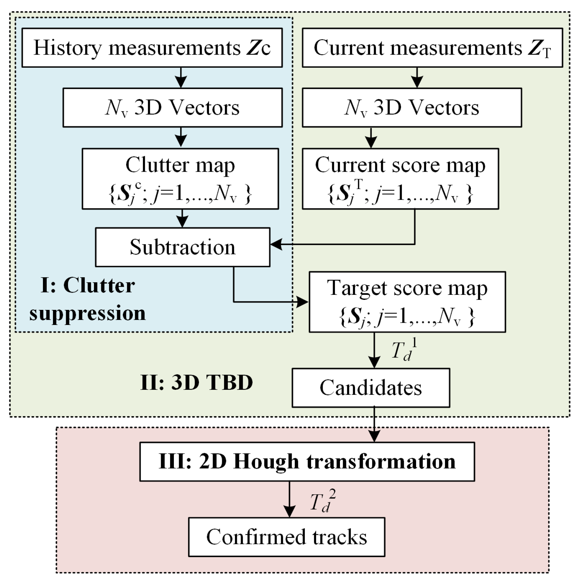
The proposed method consists of three parts, clutter suppression, 3D TBD, and 2D HT. The processing flowchart is presented in Figure 1. The three components are highlighted by blue, green, and red boxes. Firstly, $N_v$ detection bins are built [21], each detection bin corresponding to a 3D vector. In [2,19,21], the 3 dimensions in 3D TBD regard the X axis, Y axis, and time, respectively. A total of 140 3D vectors are selected for the limitation of target velocity [2]. However, the three dimensions here are the X axis, Y axis, and Z axis. Without the limitation of the target motion model, 1217 3D vectors covering all directions are exploited, and 1217 detection bins are built. The 3D vectors are built based on tessellation of Platonic solids in [32].

In clutter suppression, history measurements are firstly rotated and then projected to get a score map. Clutter density of background and clutter regions in the detection bin is denoted by the score map, so we called the score map “clutter map”. Each detection bin corresponds to one clutter map, and 1217 clutter maps are obtained in total. Then, in track detection processing, the current measurements are rotated by the same 3D vector and generate a current score map in the same way. In each detection bin, the current score map is subtracted by the clutter map. The reserved votes are regarded as target votes. The 3D TBD method introduced the 3D rotation, voting strategy for maps, and backtrace for the candidates whose score exceeds threshold $T_d^1$.

In the third part, each candidate contains one track at most. Therefore, three HT are performed on X-axis versus time, Y-axis versus time and Z-axis versus time respectively. The intersection of the point set obtained by the 3 Hough transformations is tested with the second threshold $T_d^2$. The intersection is confirmed as a target track if its score is larger than $T_d^2$. In maneuvering target tracking scenarios, tracklets can be detected by the proposed method firstly, and the whole trajectory can be then obtained by associating the tracklets [21,33].

3.2. Clutter Region Suppression

The acquisition during a long period, ${\mathit{Z}}_{\mathrm{c}}=\{x_i,y_i,z_i,t_i,w_i|i=1,\cdots ,N_{\mathrm{c}};t_1^C\le t_i\le t_2^C\}$, is exploited to estimate the effect of clutter regions and background noise. $(t_1^C,t_2^C)$ means the time window of clutter points. $N_{\mathrm{v}}$ 3D vectors are built, $\left\{\left(e_j^{\mathrm{x}},e_j^{\mathrm{y}},e_j^{\mathrm{z}}\right)|j=1,\cdots ,N_{\mathrm{v}}\right\}$. Then, the projection points $\{{\dot{x}}_i^j,{\dot{y}}_i^j,{\dot{z}}_i^j,t_i,w_i|i=1,\cdots ,N_{\mathrm{c}}\}$ can be obtained by:

$$\left\{\begin{array}{cc}\hfill & {\dot{x}}_i^j=({\left(e_j^{\mathrm{y}}\right)}^2+{\left(e_j^{\mathrm{z}}\right)}^2)x_i-\left(e_j^{\mathrm{x}}\right)\frac{\left(e_j^{\mathrm{y}}\right)y_i+\left(e_j^{\mathrm{z}}\right)z_i}{{\left(e_j^{\mathrm{x}}\right)}^2+{\left(e_j^{\mathrm{y}}\right)}^2+{\left(e_j^{\mathrm{z}}\right)}^2}\hfill \\ \hfill & {\dot{y}}_i^j=({\left(e_j^{\mathrm{x}}\right)}^2+{\left(e_j^{\mathrm{z}}\right)}^2)y_i-\left(e_j^{\mathrm{y}}\right)\frac{\left(e_j^{\mathrm{x}}\right)x_i+\left(e_j^{\mathrm{z}}\right)z_i}{{\left(e_j^{\mathrm{x}}\right)}^2+{\left(e_j^{\mathrm{y}}\right)}^2+{\left(e_j^{\mathrm{z}}\right)}^2}\hfill \\ \hfill & {\dot{z}}_i^j=({\left(e_j^{\mathrm{x}}\right)}^2+{\left(e_j^{\mathrm{y}}\right)}^2)z_i-\left(e_j^{\mathrm{z}}\right)\frac{\left(e_j^{\mathrm{x}}\right)x_i+\left(e_j^{\mathrm{y}}\right)y_i}{{\left(e_j^{\mathrm{x}}\right)}^2+{\left(e_j^{\mathrm{y}}\right)}^2+{\left(e_j^{\mathrm{z}}\right)}^2}\hfill \end{array}\right.$$

(7)

Rotation of the projected points is performed along the Z axis by ${\alpha }^j$, and ${\alpha }^j=arctan\left(\frac{e_j^{\mathrm{x}}}{e_j^{\mathrm{y}}}\right)$. Then, the rotated point $\left({\ddot{x}}_i^j,{\ddot{y}}_i^j,{\ddot{z}}_i^j\right)$ can be obtained by

$$\left(\begin{array}{c}{\ddot{x}}_i^j\\ {\ddot{y}}_i^j\\ {\ddot{z}}_i^j\end{array}\right)=\left(\begin{array}{ccc}cos\left({\alpha }^j\right)& -sin\left({\alpha }^j\right)& 0\\ sin\left({\alpha }^j\right)& cos\left({\alpha }^j\right)& 0\\ 0& 0& 1\end{array}\right)\left(\begin{array}{c}{\dot{x}}_i^j\\ {\dot{y}}_i^j\\ {\dot{z}}_i^j\end{array}\right)$$

(8)

Then, the above points are rotated again along the X axis by ${\beta }^j=arctan\left(\frac{\sqrt{{\left(e_j^{\mathrm{x}}\right)}^2+{\left(e_j^{\mathrm{y}}\right)}^2}}{e_j^{\mathrm{z}}}\right)$. The points after the above two rotations $\left({\widehat{x}}_i^j,{\widehat{y}}_i^j,{\widehat{z}}_i^j\right)$ are calculated by

$$\left(\begin{array}{c}{\widehat{x}}_i^j\\ {\widehat{y}}_i^j\\ {\widehat{z}}_i^j\end{array}\right)=\left(\begin{array}{ccc}1& 0& 0\\ 0& cos\left({\beta }^j\right)& -sin\left({\beta }^j\right)\\ 0& sin\left({\beta }^j\right)& cos\left({\beta }^j\right)\end{array}\right)\left(\begin{array}{c}{\ddot{x}}_i^j\\ {\ddot{y}}_i^j\\ {\ddot{z}}_i^j\end{array}\right)$$

(9)

The clutter map corresponding to the 3D vector $\left(e_j^{\mathrm{x}},e_j^{\mathrm{y}},e_j^{\mathrm{z}}\right)$ can be represented by ${\mathbf{S}}_j^{\mathrm{c}}$, ${\mathbf{S}}_j^{\mathrm{c}}=\{S_j^{\mathrm{c}}(m,n),m=1,2,\cdots ,N_j^{\mathrm{x}};n=1,2,\cdots ,N_j^{\mathrm{y}}\}$. The size of clutter map ${\mathbf{S}}_j^{\mathrm{c}}$ is calculated by

$$\begin{array}{cc}& N_j^{\mathrm{x}}=⌈\frac{{\widehat{x}}_{\max }^j-{\widehat{x}}_{\min }^j}{w_{xy}}⌉\hfill \\ & N_j^{\mathrm{y}}=⌈\frac{{\widehat{y}}_{\max }^j-{\widehat{y}}_{\min }^j}{w_{xy}}⌉\hfill \end{array}$$

(10)

The ${\widehat{x}}_{\max }^j$ and ${\widehat{x}}_{\min }^j$ denote the maximum and minimum value of the rotated point set. So does the ${\widehat{y}}_{\max }^j$ and ${\widehat{y}}_{\max }^j$.

$$\begin{array}{cc}& {\widehat{x}}_{\max }^j=max\left(\left\{{\widehat{x}}_i^j|1,\dots ,N_{\mathrm{c}}\right\}\right);{\widehat{x}}_{\min }^j=min\left(\left\{{\widehat{x}}_i^j|1,\dots ,N_{\mathrm{c}}\right\}\right)\hfill \\ & {\widehat{y}}_{\max }^j=max\left(\left\{{\widehat{y}}_i^j|1,\dots ,N_{\mathrm{c}}\right\}\right);{\widehat{y}}_{\min }^j=min\left(\left\{{\widehat{y}}_i^j|1,\dots ,N_{\mathrm{c}}\right\}\right)\hfill \end{array}$$

(11)

The $N_c$ points $\left\{\left({\widehat{x}}_i^j,{\widehat{y}}_i^j,{\widehat{z}}_i^j,w_i|i=1,\cdots ,N_c\right)\right\}$ vote for the clutter map ${\mathbf{S}}_j^{\mathrm{c}}$ by

$$s_j^{\mathrm{c}}\left(x,y\right)=\frac{{\sum }_{i=1}^{N_{\mathrm{c}}}{I}_3(x,y)w_i}{t_1^{\mathrm{c}}-t_2^{\mathrm{c}}}$$

(12)

$$I_3(x,y)=\left(\begin{array}{cc}& 1;x=\left[\frac{{\widehat{x}}_i^j-{\widehat{x}}_{\min }^j}{w_{xy}}\right];y=\left[\frac{{\widehat{y}}_i^j-{\widehat{y}}_{\min }^j}{w_{xy}}\right]\hfill \\ & 0;\mathrm{Otherwise}\hfill \end{array}\right.$$

(13)

The clutter map set $\left\{{\mathbf{S}}_j^{\mathrm{c}}\right|j=1,\cdots ,N_{\mathrm{v}}\}$ is designed to cancel the component of the clutter region in the projected map.

3.3. The 4D TBD

After obtaining the clutter map in $N_v$ detection bins, we detect the current tracks by the latest measurements. The latest measurement point set is represented by $\mathit{Z}=\{x_i,y_i,z_i,t_i,w_i|i=1,\cdots ,N;t_1^T\le t_i\le t_2^T\left\}\right\}$. $(t_1^T,t_2^T)$ denote the time window in which the target track exists. The $\mathit{Z}$ is also rotated by $N_v$ 3D vectors in each detection bin. Each detection bin generates a current projected map. Corresponding to the $N_v$ clutter map, the $N_v$ current projected map is represented by $\left\{{\mathbf{S}}_j^{\mathrm{T}}\right|j=1,\cdots ,N_{\mathrm{v}}\}$. Current projected map ${\mathbf{S}}_j^{\mathrm{T}}$ is obtained by (7)–(9) and (12) using measurements $\mathit{Z}$.

Then, we can get the projected map after clutter region suppression, $\left\{{\mathbf{S}}_j\right|j=1,\cdots ,N_{\mathrm{v}}\}$, by subtraction of the two maps.

$${\mathbf{S}}_j=\left\{S_j(m,n)\right|m=1,\cdots ,N_j^{\mathrm{x}};n=1,\cdots ,N_j^{\mathrm{y}}\}$$

(14)

$$S_j(m,n)=S_j^{\mathrm{T}}(m,n)-S_j^{\mathrm{c}}(m,n)$$

(15)

Then the cells whose score is larger than a threshold $T_{\mathrm{d}}^1$ in map $\left\{{\mathbf{S}}_j\right\}$ are found out. These cells are candidates potentially containing a target track. Therefore, these cells are called “candidate cell”. If all the cells in $\left\{{\mathbf{S}}_j\right\}$ are smaller than the $T_{\mathrm{d}}^1$, it infers that no target whose direction close to the 3D vector of this detection bin exists. It is unnecessary to do further processing on this detection bin.

The candidate cells in the same score map are firstly clustered into sets to get the candidate regions by the region growing method in [33,34]. Each candidate cell set potentially contains a target track. It assumes that $N_j$ candidate regions are obtained in the ${\mathbf{S}}_j$. Further detection will be performed on each set. The cardinality of a candidate cell set is denoted by $N_j^r$. Candidate region set ${\mathbf{R}}_j$ can be expressed by

$$\begin{array}{cc}\hfill {\mathbf{R}}_j& =\left\{{\mathbf{R}}_j^r\right|r=1,\dots ,N_j\}\hfill \\ \hfill {\mathbf{R}}_j^r& =\{S_j^r(m_a,n_a)>T_{\mathrm{d}}^1|a=1,\dots ,N_j^r\}\hfill \end{array}$$

(16)

The processing of each region in $\left\{{\mathbf{S}}_j\right\}$ follows three steps.

Firstly, the points voting for the candidate cell set are backtracked. The 3D straight line which corresponds to a candidate cell $S_j(m_a,n_a)$ can be expressed by

$$\frac{x-(m_a{w}_{\mathrm{xy}}-{\widehat{x}}_{\min }^j)}{e_j^{\mathrm{x}}}=\frac{y-(m_b{w}_{\mathrm{xy}}-{\widehat{y}}_{\min }^j)}{e_j^{\mathrm{y}}}=\frac{z}{e_j^{\mathrm{z}}}$$

(17)

If the distance $d_i^j(m_a,n_a)$ between the 3D line (17) and a rotated point $\left({\widehat{x}}_i^j,{\widehat{y}}_i^j,{\widehat{z}}_i^j\right)$ is smaller than cell width $w_{\mathrm{xy}}$, the point $\left({\widehat{x}}_i^j,{\widehat{y}}_i^j,{\widehat{z}}_i^j\right)$ should vote for the cell $S_j(m_a,n_a)$. The expressions for the distance $d_i^j(m_a,n_a)$ are available in [19]. The point set voting for the $S_j(m_a,n_a)$ is denoted by ${\mathit{Z}}_j(m_a,n_a)=\left\{\left({\widehat{x}}_i^j,{\widehat{y}}_i^j,{\widehat{z}}_i^j\right)|i=1,\cdots ,N_j(m_a,n_a)\right\}$. Then, the corresponding point set of the candidate region ${\mathit{Z}}_j^r$ can be expressed by the union of $N_j^{\mathrm{c}}$ point set, i.e.,

$${\mathit{Z}}_j^r={\mathit{Z}}_j(m_1,n_1)\bigcup \cdots \bigcup {\mathit{Z}}_j(m_{N_j^{\mathrm{c}}},n_{N_j^{\mathrm{c}}})$$

(18)

The parameter r denotes the index of the candidate regions in ${\mathbf{S}}_j$. Each set ${\mathit{Z}}_j^r$ is promising and contains one track.

Secondly, three 2D HT are performed according to (1). On the X axis, a parameter space map of $(x_0^k,v_{\mathrm{x}}^k)$ is built. The parameter space map has $N_{\mathrm{H}}^0$ bins for $x_0^k$ and $N_{\mathrm{H}}^{\mathrm{V}}$ bins for $v_{\mathrm{x}}^k$. The parameter space map can be denoted by ${\mathbf{S}}_{j,\mathrm{x}}^r=\left\{S_{j,\mathrm{x}}^r(x,y)\right|x=1,\cdots ,N_{\mathrm{H}}^0;y=1,\cdots ,N_{\mathrm{H}}^{\mathrm{V}}\}$. The bin width of $x_0^k$ and $v_{\mathrm{x}}^k$ is $w_{\mathrm{H}}^0$ and $w_{\mathrm{x}}^k$, respectively. The voting process corresponding to the X axis can be expressed by

$$S_{j,\mathrm{x}}^r\left(x,y\right)=\sum _{i=1}^{|{\mathit{Z}}_j^r|}{I}_2(x,y)w_i$$

(19)

$$I_2(x,y)=\left(\begin{array}{c}1;x=\left[\frac{{\widehat{y}}_i^j-{\widehat{x}}_i^j{w}_{\mathrm{x}}^{k}y}{w_{\mathrm{H}}^0}\right]\hfill \\ 0;\mathrm{Otherwise}\hfill \end{array}\right.$$

(20)

The maximum score of parameter space map, $M_{j,\mathrm{x}}^r$, can be obtained by enumeration. Similarly, on the Y axis and Z axis, 2D HT is also performed for the $M_{j,\mathrm{y}}^r$ and $M_{j,\mathrm{z}}^r$. If all three maximums, $M_{j,\mathrm{x}}^r$,$M_{j,\mathrm{y}}^r$, and $M_{j,\mathrm{Z}}^r$, are larger than a fixed threshold $T_{\mathrm{d}}^2$, we believe that one track exits in the point set ${\mathit{Z}}_j^r$, i.e.,

$$\left\{\begin{array}{c}\hfill M_{j,\mathrm{x}}^r>T_{\mathrm{d}}^2\\ \hfill M_{j,\mathrm{y}}^r>T_{\mathrm{d}}^2\\ \hfill M_{j,\mathrm{z}}^r>T_{\mathrm{d}}^2\end{array}\right.\Rightarrow \mathrm{Target}\mathrm{track}\mathrm{confirmed}$$

(21)

The points which were voting for the cell of maximum vote $M_{j,\mathrm{x}}^r$ are represented by ${\mathbf{T}}_j^{r,\mathrm{x}}$. Similarly, we can get the point sets ${\mathbf{T}}_j^{r,\mathrm{y}}$ and ${\mathbf{T}}_j^{r,\mathrm{z}}$. The obtained tracklet in ${\mathbf{T}}_j^r$ is exactly the intersection of the three point set, i.e.,

$${\mathbf{T}}_j^r={\mathbf{T}}_j^{r,\mathrm{x}}\bigcap {\mathbf{T}}_j^{r,\mathrm{y}}\bigcap {\mathbf{T}}_j^{r,\mathrm{z}}$$

(22)

Thirdly, track fusion is necessary to avoid duplicate detection. The same track may be detected in more than one detection bin if 3D vectors of detection bins are very close. Therefore, if two 3D vectors, $\left(e_{j_1}^{\mathrm{x}},e_{j_1}^{\mathrm{y}},e_{j_1}^{\mathrm{z}}\right)$ and $\left(e_{j_2}^{\mathrm{x}},e_{j_2}^{\mathrm{y}},e_{j_2}^{\mathrm{z}}\right)$, meet the expression in (23), the tracks detected in the two detection bins are attempted for fusion.

$$arccos\left(e_{j_1}^{\mathrm{x}}{e}_{j_2}^{\mathrm{x}}+e_{j_1}^{\mathrm{y}}{e}_{j_2}^{\mathrm{y}}+e_{j_1}^{\mathrm{z}}{e}_{j_2}^{\mathrm{z}}\right)<T_{\mathrm{f}}$$

(23)

The $T_{\mathrm{f}}$ is a constant set to $\frac{\pi }{15}$ in our experiments. Each pair of the tracklets obtained in $j_1$-th and $j_2$-th detection bins are compared. Two tracks are fused if they are sharing the same points, and the fusion can be expressed by (24)

$$\left|{\mathbf{T}}_{j_1}^r\bigcup {\mathbf{T}}_{j_2}^r\right|>\eta min\left\{\left|{\mathbf{T}}_{j_1}^r\right|,\left|{\mathbf{T}}_{j_1}^r\right|\right\}⟹{\mathbf{T}}_j^r={\mathbf{T}}_{j_1}^r\bigcap {\mathbf{T}}_{j_2}^r$$

(24)

where the constant parameter $\eta$ is set to 0.5 in the experiments.

3.4. Theoretical Model

After the introduction of methods in each stage, an integrated theoretical model of the whole algorithm is given.

The measurements during a time period are projected, rotated firstly. Then, a map voted by the rotated points is obtained in each detection bin. Each map contains $N_j^{\mathrm{x}}\times N_j^{\mathrm{Y}}$ grid cells which are sized $w_{\mathrm{xy}}\times w_{\mathrm{xy}}$. The votes in a map cell consist of three parts when a track exists, i.e., the votes of the target, background, and clutter region. The expectation of the three components all follow a Poisson distribution, and their expectation is

$$\frac{t_2^T-t_1^T}{t_{\mathrm{In}}}\times {\gamma }_k\Rightarrow \mathrm{Target}$$

(25)

$$(t_2^T-t_1^T)\left(w_{\mathrm{xy}}{w}_{\mathrm{xy}}{R}_{\mathrm{C}}\right){\gamma }_0\Rightarrow \mathrm{Background}\mathrm{clutter}$$

(26)

$$(t_2^T-t_1^T)\left(w_{\mathrm{xy}}{w}_{\mathrm{xy}}{R}_{\mathrm{C}}{I}_3(x,y)\right){\gamma }_c^0\Rightarrow \mathrm{Clutter}\mathrm{region}$$

(27)

The $R_{\mathrm{C}}$ means the radar coverage range. The historical measurement ${\mathit{Z}}_{\mathrm{c}}$ is exactly used to estimate the clutter components, i.e., (26) and (27). The clutter components in each grid cell and in $N_{\mathrm{v}}$ detection bins ($\left\{{\mathbf{S}}_j^{\mathrm{c}}\right|j=1,\cdots ,N_{\mathrm{v}}\}$) are estimated by (7)–(12).

If a target exists in a cell, the expectation of the points voting for the cell is the summation of (25) and (26) (target not in a clutter region) or the summation of (25)–(27) (target in a clutter region). The map is precisely the ${\mathbf{S}}_j^{\mathrm{T}}$, which is estimated by $\mathit{Z}$ by using (7)–(12).

In ${\mathbf{S}}_j^{\mathrm{c}}$ and ${\mathbf{S}}_j^{\mathrm{T}}$, the distributions of false alarm points in each cell generated by background (26) and clutter regions (27) are the same, as the variation of clutter is quite slow compared with that of the target cell. Therefore, after the subtraction of ${\mathbf{S}}_j^{\mathrm{c}}$ and ${\mathbf{S}}_j^{\mathrm{T}}$ (15), only the components of target (25) are reserved in ${\mathbf{S}}_j$, and it is much larger than the residual error of subtraction in (15). Therefore, target detection in ${\mathbf{S}}_j$ is quite easy, and the subtraction in each detection bin is the theoretical basis of our improvements.

The distribution of the quantity of the points in a target cell can be expressed by (28) because the summation of several individual Poisson processes also follows a Poisson distribution.

$$\begin{array}{cc}\hfill P_{\mathrm{t}}\left(n\right)& =\frac{{\left({\gamma }_{\mathrm{t}}^{3\mathrm{D}}\right)}^n}{n!}\times e^{-{\gamma }_{\mathrm{t}}^{3\mathrm{D}}};n=0,1,\dots ,\infty \hfill \\ & {\gamma }_{\mathrm{t}}^{3\mathrm{D}}=(t_2^T-t_1^T)(\frac{{\gamma }_k}{t_{\mathrm{In}}}+\left(w_{\mathrm{xy}}{w}_{\mathrm{xy}}{R}_{\mathrm{C}}\right)({\gamma }_0+I_3(x,y){\gamma }_c^0))\hfill \end{array}$$

(28)

Similarly, the distribution of a cell in which a target is absent can be written as

$$\begin{array}{cc}\hfill P_{\mathrm{c}}\left(n\right)& =\frac{{\left({\gamma }_{\mathrm{c}}^{3\mathrm{D}}\right)}^n}{n!}\times e^{-{\gamma }_{\mathrm{c}}^{3\mathrm{D}}};n=0,1,\dots ,\infty \hfill \\ & {\gamma }_{\mathrm{c}}^{3\mathrm{D}}=(t_2^T-t_1^T)\left(w_{\mathrm{xy}}{w}_{\mathrm{xy}}{R}_{\mathrm{C}}\right)({\gamma }_0+I_3(x,y){\gamma }_c^0)\hfill \end{array}$$

(29)

The vote of cell in clutter map $S_j^{\mathrm{c}}(x,y)$ is the expectation of clutter components, i.e., $S_j^{\mathrm{c}}(x,y)=(t_2^T-t_1^T)\left(w_{\mathrm{xy}}{w}_{\mathrm{xy}}{R}_{\mathrm{C}}({\gamma }_0+I_3(x,y){\gamma }_c^0)\right)$. If the threshold equals $T_d^1$, the false alarm detection probability of a cell $(x,y)$ can be written as

$$P_{\mathrm{FA}}^{3\mathrm{D}}\left(T_d^1\right)=\sum _{n={\gamma }_{\mathrm{c}}^{3\mathrm{D}}+T_d^1}^{\infty }{P}_{\mathrm{c}}\left(n\right)$$

(30)

The false alarm rate is the summation of the probability of votes more than ${\gamma }_{\mathrm{c}}^{3\mathrm{D}}+T_d^1$. According to (30), the estimated clutter $S_j^{\mathrm{c}}(x,y)$ and the component ${\gamma }_{\mathrm{c}}^{3\mathrm{D}}$ in (29) are canceled out. Therefore, the summation is usually very low in using an appropriate $T_d^1$.

According to (28), the detection rate can be written as

$$P_{\mathrm{D}}^{3\mathrm{D}}\left(T_d^1\right)=\sum _{n={\gamma }_{\mathrm{c}}^{3\mathrm{D}}+T_d^1}^{\infty }{P}_{\mathrm{t}}\left(n\right)$$

(31)

For the contribution of target component, $(t_2^T-t_1^T)\left(\frac{{\gamma }_k}{t_{\mathrm{In}}}\right)$, exceeding ${\gamma }_{\mathrm{c}}^{3\mathrm{D}}+T_d^1$ is quite easy for the ${\gamma }_{\mathrm{t}}^{3\mathrm{D}}$. It provides a remarkable detection rate of the target tracklet.

Even if a false alarm tracklet is built by the 3D HT, three 2D HT are performed to further verify the tracklet. In the 2D HT, the parameter space is divided into $H_{\mathrm{H}}^0\times H_{\mathrm{H}}^{\mathrm{V}}$ grid cells. Each point would vote for all $H_{\mathrm{H}}^{\mathrm{V}}$ speed bins in 2D Hough map ${\mathbf{S}}_{j,\mathrm{x}}^r$, each velocity bin one vote. Therefore, the map ${\mathbf{S}}_{j,\mathrm{x}}^r$ has $|{\mathit{Z}}_j^r|\times H_{\mathrm{H}}^{\mathrm{V}}$ votes in total. If a cell has been correctly confirmed as a tracklet candidate, it contains $(t_2-t_1)\left(w_{\mathrm{xy}}{w}_{\mathrm{xy}}{R}_{\mathrm{C}}\right)({\gamma }_0+I_3(x,y){\gamma }_c^0)+T_d^1$ points, at least. The point cardinality of the set ${\mathit{Z}}_j^r$ follows the distribution:

$$\begin{array}{cc}\hfill P_{2\mathrm{t}}\left(n\right)& =\frac{\frac{{\left({\gamma }_{\mathrm{t}}^{3\mathrm{D}}\right)}^n}{n!}\times e^{-{\gamma }_{\mathrm{t}}^{3\mathrm{D}}}}{{\displaystyle \sum _{n=⌈{\gamma }_{\mathrm{t}}^{3\mathrm{D}}+T_{d,\mathrm{opt}}^1⌉}^{\infty }}{P}_{\mathrm{t}}\left(n\right)};n=⌈{\gamma }_{\mathrm{t}}^{3\mathrm{D}}+T_{d,\mathrm{opt}}^1⌉,\dots ,\infty \hfill \end{array}$$

(32)

Similarly, the point cardinality of set $|{\mathit{Z}}_j^r|$ in which no target points exist but has been falsely confirmed as a candidate follows the distribution:

$$\begin{array}{cc}\hfill P_{2\mathrm{c}}\left(n\right)& =\frac{\frac{{\left({\gamma }_{\mathrm{c}}^{3\mathrm{D}}\right)}^n}{n!}\times e^{-{\gamma }_{\mathrm{c}}^{3\mathrm{D}}}}{{\displaystyle \sum _{n=⌈{\gamma }_{\mathrm{c}}^{3\mathrm{D}}+T_{d,\mathrm{opt}}^1⌉}^{\infty }}{P}_{\mathrm{c}}\left(n\right)};n=⌈{\gamma }_{\mathrm{c}}^{3\mathrm{D}}+T_{d,\mathrm{opt}}^1⌉,\dots ,\infty \hfill \end{array}$$

(33)

If the clutter points randomly vote for the $H_{\mathrm{H}}^0\times H_{\mathrm{H}}^{\mathrm{V}}$ cells in map ${\mathbf{S}}_{j,\mathrm{x}}^r$, the expectation of vote in each cell can be expressed by

$$\frac{{\gamma }_{\mathrm{c}}^{3\mathrm{D}}+T_{d,\mathrm{opt}}^1}{H_{\mathrm{H}}^0}$$

(34)

According to (33), the vote distribution of a cell in map ${\mathbf{S}}_{j,\mathrm{x}}^r$ if no target exits can be expressed by

$$\begin{array}{cc}\hfill P_{2\mathrm{c}}^{\mathrm{x}}\left(n\right)& =\frac{\frac{{\left({\gamma }_{\mathrm{c}}^{2\mathrm{D}}\right)}^n}{n!}\times e^{-{\gamma }_{\mathrm{c}}^{2\mathrm{D}}}}{{\displaystyle \sum _{n=⌈{\gamma }_{\mathrm{c}}^{3\mathrm{D}}+T_{d,\mathrm{opt}}^1⌉}^{\infty }}{P}_{\mathrm{c}}\left(n\right)};n=0,\dots ,\infty \hfill \\ & {\gamma }_{\mathrm{c}}^{2\mathrm{D}}=\frac{{\gamma }_{\mathrm{c}}^{3\mathrm{D}}+T_{d,\mathrm{opt}}^1}{H_{\mathrm{H}}^0}\hfill \end{array}$$

(35)

Then, the false alarm rate of $T_d^2$ in map ${\mathbf{S}}_{j,\mathrm{x}}^r$ can be written as

$$P_{\mathrm{FA}}^{2\mathrm{D},\mathrm{x}}\left(T_d^2\right)=\sum _{n={\gamma }_{\mathrm{c}}^{2\mathrm{D}}+T_d^2}^{\infty }{P}_{2\mathrm{c}}^{\mathrm{x}}\left(n\right)$$

(36)

Similarly, the distributions $P_{\mathrm{FA}}^{2\mathrm{D},\mathrm{y}}\left(T_d^2\right)$ and $P_{\mathrm{FA}}^{2\mathrm{D},\mathrm{z}}\left(T_d^2\right)$, which correspond to ${\mathbf{S}}_{j,\mathrm{y}}^r$ and ${\mathbf{S}}_{j,\mathrm{z}}^r$, are available, and the three distributions are individual with each other. Therefore, according to (21), the overall false alarm rate of track detection can be expressed by

$$P_{\mathrm{FA}}^{2\mathrm{D}}\left(T_d^2\right)=P_{\mathrm{FA}}^{2\mathrm{D},\mathrm{x}}\left(T_d^2\right)\times P_{\mathrm{FA}}^{2\mathrm{D},\mathrm{y}}\left(T_d^2\right)\times P_{\mathrm{FA}}^{2\mathrm{D},\mathrm{z}}\left(T_d^2\right)$$

(37)

The $P_{\mathrm{FA}}^{2\mathrm{D},\mathrm{x}}\left(T_d^2\right)$ is usually very low because the score is hard to exceed $T_d^2$ if the point set originates from clutter and the points are randomly voting for the cells. Meanwhile, according to (37), even if the false alarm arises in one 2D HT map, the false alarm track is very hard to pass the three 2D HT map detection at the same time. Therefore, (36) and (37) grant our method an extremely low false track detection rate.

If the target points exist in a cell, the clutter points randomly vote for the $H_{\mathrm{H}}^0\times H_{\mathrm{H}}^{\mathrm{V}}$ cells in map ${\mathbf{S}}_{j,\mathrm{x}}^r$. However, all the target points would vote for the one cell, and the vote expectation of the cell can be expressed by

$$\frac{{\gamma }_{\mathrm{c}}^{3\mathrm{D}}+T_{d,\mathrm{opt}}^1}{H_{\mathrm{H}}^0}+\frac{{\gamma }_k}{t_{\mathrm{In}}}$$

(38)

According to (32), the distribution of votes in a cell of map ${\mathbf{S}}_{j,\mathrm{x}}^r$ when the target actually exists can be expressed by

$$\begin{array}{cc}\hfill P_{2\mathrm{t}}^{\mathrm{x}}\left(n\right)& =\frac{\frac{{\left({\gamma }_{\mathrm{t}}^{2\mathrm{D}}\right)}^n}{n!}\times e^{-{\gamma }_{\mathrm{t}}^{2\mathrm{D}}}}{{\displaystyle \sum _{n=⌈{\gamma }_{\mathrm{t}}^{3\mathrm{D}}+T_{d,\mathrm{opt}}^1⌉}^{\infty }}{P}_{\mathrm{t}}\left(n\right)};n=0,\dots ,\infty \hfill \\ & {\gamma }_{\mathrm{t}}^{2\mathrm{D}}=\frac{{\gamma }_{\mathrm{c}}^{3\mathrm{D}}+T_{d,\mathrm{opt}}^1}{H_{\mathrm{H}}^0}+\frac{{\gamma }_k}{t_{\mathrm{In}}}\hfill \end{array}$$

(39)

The detection rate of $T_d^2$ in map ${\mathbf{S}}_{j,\mathrm{x}}^r$ can be written as

$$P_{\mathrm{D}}^{2\mathrm{D},\mathrm{x}}\left(T_d^2\right)=\sum _{n={\gamma }_{\mathrm{t}}^{2\mathrm{D}}+T_d^2}^{\infty }{P}_{2\mathrm{t}}^{\mathrm{x}}\left(n\right)$$

(40)

According to (21), the track can be confirmed only if it is detected in all three 2D Hough maps. Therefore, the overall track detection rate can be expressed by

$$P_{\mathrm{D}}^{2\mathrm{D}}=P_{\mathrm{D}}^{2\mathrm{D},\mathrm{x}}\left(T_d^2\right)\times P_{\mathrm{D}}^{2\mathrm{D},\mathrm{y}}\left(T_d^2\right)\times P_{\mathrm{D}}^{2\mathrm{D},\mathrm{z}}\left(T_d^2\right)$$

(41)

For the component of target points, $\frac{{\gamma }_k}{t_{\mathrm{In}}}$, the vote is very easy to exceed $T_d^2$, and the $P_{\mathrm{D}}^{2\mathrm{D},\mathrm{x}}\left(T_d^2\right)$ is close to 1. Similarly, a high detection rate of target track $P_{\mathrm{D}}^{2\mathrm{D}}$ can be achieved.

3.5. Implementation of the Whole Algorithm

The implementation of the proposed method is explained by the Pseudocode in Algorithm 1. In the Pseudocode, lines 1–3 present the clutter map ${\mathbf{S}}_j^{\mathrm{c}}$ estimation using ${\mathit{Z}}_{\mathrm{c}}$ in $N_v$ detection bins. In lines 5 and 6, target map ${\mathbf{S}}_j$ is calculated, and only the component of target (25) is reserved. In line 7, $N_j$ target regions are easily obtained. In lines 9–12, three 2D HT are performed. In lines 13–15, the target tracklet is confirmed. After getting all the tracklets in $N_v$ detection bins in lines 4–17, tracklet fusion is performed in line 18.

A diagram presenting the whole process is given in Figure 2 to make our method more understandable. The two sub-figures in the first line present the measurement points $\mathit{Z}$ in the example and the 3D vectors $\left(e_j^{\mathrm{x}},e_j^{\mathrm{y}},e_j^{\mathrm{z}}\right)$. They are the inputs to detect the four target tracklets. The measurements include the target points and false alarm points originating in the background and two clutter regions. The weight of all points is the same at the beginning. The target points are labeled by larger balls for distinction. The blue to red points denote the initial points to most recently obtained points. In the second line, three 3D vectors are presented as examples. Each vector regards a detection bin. In the third line, points after projection (7) and two rotation (8) and (9), i.e., $\left({\widehat{x}}_i^j,{\widehat{y}}_i^j,{\widehat{z}}_i^j\right)$, in the three detection bins are presented. In the first detection bin, one target track is perpendicular to the current X-Y plane. Two target tracks are perpendicular to the plane in the subfigure in line 3, column 2. In the fourth line, the score maps before clutter suppression ${\mathbf{S}}_j^{\mathrm{T}}$ in the three detection bins are presented. The vote of two clutter regions is quite outstanding. The clutter map ${\mathbf{S}}_j^{\mathrm{c}}$, which is built by history measurements ${\mathit{Z}}_{\mathrm{c}}$, is presented by the subfigures in the fifth line. Subfigures in the sixth line and seventh line present the projected map when the false alarm points are absent and present, respectively. In the projected map ${\mathbf{S}}_j$, the target region is much easier to be detected. The target region in the first detection bin is outstanding in subfigure of line 7, column 1. The points in set ${\mathit{Z}}_1^1$, which vote for the target region, are presented in the subfigure of line 8, column 1. Then, one tracklet can be obtained after 2D HT in the subfigure of line 9, column 1. Similarly, in the second detection bin, two target regions are detected in the subfigures of line 7, column 2. Two tracklets can be then obtained after two individual 2D HT processing. In the third column ($j\mathrm{th}$ detection bin), no target regions can be obtained in subfigures of line 7, column 3. That means no tracklet can be obtained in this detection bin. The subfigures in the bottom (line 10) present all the tracklets obtained by the $N_{\mathrm{v}}$ detection bins.

Algorithm 1: The 4D Track-before-detect method.

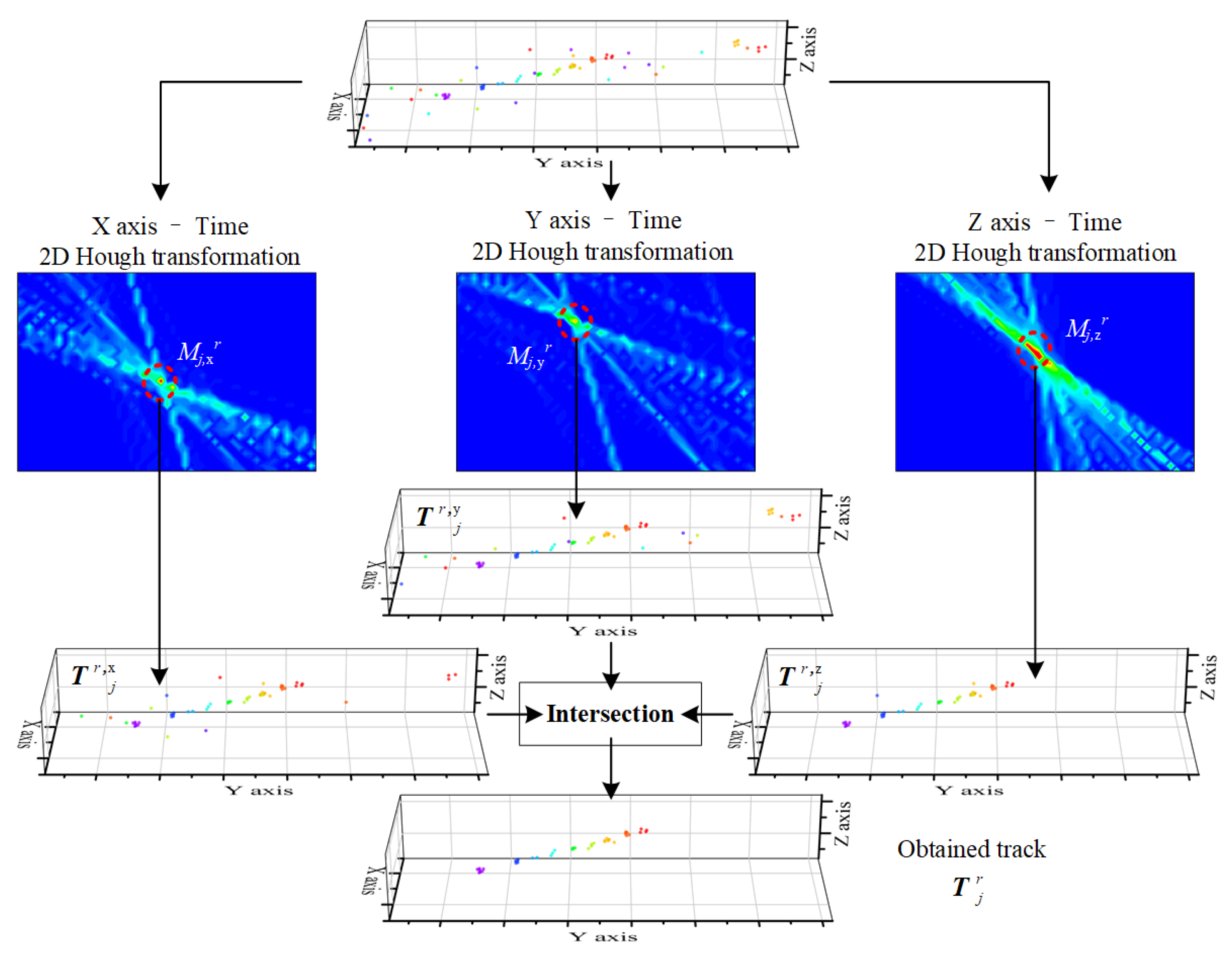
An example of 2D HT is presented in Figure 3. The subfigure in the first line presents the point set of a target region, ${\mathit{Z}}_i^r$. It shows that the point of a target tracklet and a few false alarm points exist. In the second line, the maps of HT in X axis-time, Y axis-time, and Z axis-time are present. The target region in each 2D HT map ($M_{j,\mathrm{x}}^r$, $M_{j,\mathrm{y}}^r$ and $M_{j,\mathrm{z}}^r$) is highlighted by a red circle. As is presented in the three subfigures in the third line, the points which were voting for the target region in each 2D HT map are extracted, i.e., ${\mathbf{T}}_j^{r,\mathrm{x}}$, ${\mathbf{T}}_j^{r,\mathrm{Y}}$, and ${\mathbf{T}}_j^{r,\mathrm{Z}}$. In the three point sets, both the target points and a few false alarm points are included. At the bottom of Figure 3, the intersection of three point set, also the obtained track, is presented. It shows that all the target points are detected in the track ${\mathbf{T}}_j^r$, and false alarm points have been filtered out.

3.6. Discussion of Thresholds

The tracking performance is closely related to the detection thresholds $T_d^1$ in (16) and $T_d^2$ in (21). The optimal values of the two thresholds are decided by the parameters of targets and measurement environment.

The $T_d^1$ is applied to confirm the candidate target region in the 3D voting process. The optimal threshold $T_{d,\mathrm{opt}}^1$ can be defined by (42) according to (30) and (31)

$$T_{d,\mathrm{opt}}^1=argmax\left\{P_{\mathrm{D}}^{3\mathrm{D}}\left(T_d^1\right)-P_{\mathrm{FA}}^{3\mathrm{D}}\left(T_d^1\right)\right\}$$

(42)

The track is easier to be detected if more target points and fewer clutter points are voting for the cell, i.e.,

$$(t_2-t_1)\left(\frac{{\gamma }_k}{t_{\mathrm{In}}}-w_{\mathrm{xy}}{w}_{\mathrm{xy}}{R}_{\mathrm{C}}({\gamma }_0+I_3(x,y){\gamma }_c^0)\right)\gg 0$$

(43)

In (43), $t_{\mathrm{In}}$ and $R_{\mathrm{C}}$ are the constants in the radar system. The ${\gamma }_k$, ${\gamma }_0$, and ${\gamma }_c^0$ are related to targets and measurement environment and are out of our control. The $w_{\mathrm{xy}}$ should match with the measurement position error of radar systems, otherwise not all the target points would vote for the cell. Therefore, the most simple approach to improve the target track detection performance is to enhance the time period, i.e., $(t_2-t_1)$. However, it is worth noting that the discussion in this section is built on the target model in (17). Therefore, a very large value of $(t_2-t_1)$ is unsuitable because the target may be maneuvering during $t_1$ to $t_2$. The (43) also proves that the merit of track-before-detect method comes from accumulating the target “votes” according to the target motion model during a long enough time.

The $T_d^2$ is applied to confirm the candidate target region in the 2D voting process. Similarly, the optimal threshold $T_{d,\mathrm{opt}}^2$ can be defined by

$$T_{d,\mathrm{opt}}^2=argmax\left\{P_{\mathrm{D}}^{2\mathrm{D}}\left(T_d^2\right)-P_{\mathrm{FA}}^{2\mathrm{D}}\left(T_d^2\right)\right\}$$

(44)

With using $T_{d,\mathrm{opt}}^1$ and $T_{d,\mathrm{opt}}^2$, a high target track detection rate and a very low false alarm track rate can be achieved at the same time.

4. Case Study

4.1. Synthetic Data Experiment

To fully access the superiority of the proposed algorithm, experiments using synthetic data are conducted.

4.1.1. Optimal Threshold Estimation

Before performing the tracking method, the optimal thresholds $T_{d,\mathrm{opt}}^1$ and $T_{d,\mathrm{opt}}^2$ are estimated. The parameters used in the method are presented in

Table 1. Parameters of the proposed method.

Parameter	Values
$N_v$	1217
$w_{\mathrm{xy}}$	100 m
$(t_2^C-t_1^C)$	40 s
$(t_2^T-t_1^T)$	10 s
$t_{\mathrm{In}}$	1.1 s
${\gamma }_c^0$	$15\times {10}^{-10}$
${\gamma }_k$	3
$R_C$	30 Km
$T_f$	$\pi /15$
$\gamma$	0.5
$w_{\mathrm{H}}^0$	50 m/s
$w_{\mathrm{x}}^0$	200 m
$T_{d,\mathrm{opt}}^1$	11.5
$T_{d,\mathrm{opt}}^2$	19.97

. These parameters are applied in both synthetic data and real experiments. Figure 4a presents the relationship between $T_d^1$ and $\left\{P_{\mathrm{D}}^{3\mathrm{D}}\left(T_d^1\right)-P_{\mathrm{FA}}^{3\mathrm{D}}\left(T_d^1\right)\right\}$, and that of $T_d^2$ and $\left\{P_{\mathrm{D}}^{2\mathrm{D}}\left(T_d^2\right)-P_{\mathrm{FA}}^{2\mathrm{D}}\left(T_d^2\right)\right\}$ is presented in Figure 4b. The detection performance could be remarkably good when the difference is close to 1. The curves in different colors mean using different $T_e^t$, $T_e^t=t_2^{\mathrm{T}}-t_1^{\mathrm{T}}$. A large $T_e^t$ represents more measurements are jointly processed in the time window. The curves of $T_e^t=1,\cdots ,10$ s infer that a larger time window is beneficial to achieve a better performance on weak targets. According to (42) and (44), the optimal $T_d^1$ and $T_d^2$ are 11.5 and 19.97 respectively.

4.1.2. Scenario and Parameters of Synthetic Experiment

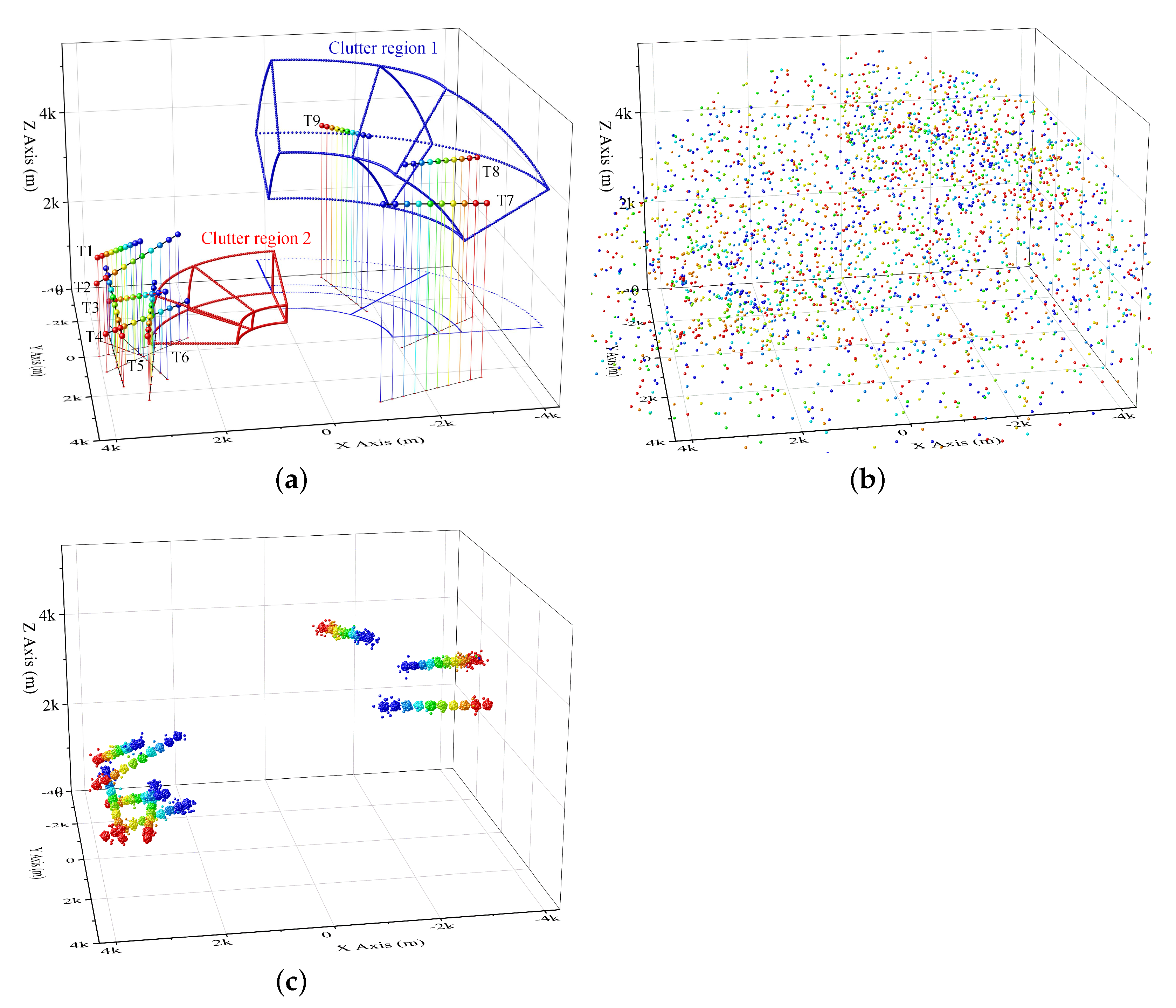
In order to numerically assess the performance of the proposed processing chain, 200 Monte Carlo numerical simulations are performed for the tracks. Figure 5a presents the simulated scenario in which 9 target tracks and 2 clutter regions exist. The time duration of the measurement is 10 scans. The 9 tracks are labeled by $\mathrm{T}1$ to $\mathrm{T}9$ and can be partitioned into 3 groups. The first group, which includes track 1 to track 6, is closely distributed tracks. The second group is merely track 7, an individual target. The third group contains track 8 and track 9. Track 8 is located at the boundary of clutter region 1. Half of track 8 is in the clutter region, and the other 5 scans are out of the clutter region. Track 9 is totally inside the clutter region. The two clutter regions, clutter region 1 and clutter region 2, are different in clutter density. Besides clutter regions, the background false alarm points also widely exist in the surveillance area. The values of simulation parameters are patched in

Table 2. Simulation parameters.

Parameter	Values
Measurement rate (${\gamma }_k$)	2.5
Measurement noise in X Y Z axis	(30, 30, 30) (m)
Background clutter density (${\gamma }_0$)	5 × 10−10 (1/m3)
Clutter region 1 density (${\gamma }_1^0$)	15 × 10−10 (1/m3)
Clutter region 2 density (${\gamma }_2^0$)	25 × 10−10 (1/m3)

.

The synthetic measurement points in an experiment during 10 scans are presented in Figure 5b. The point color represents the time information; red means the first scan, and blue means the last scan. It is hard to find the target points without an outstanding tracking method because of the massive clutter points.

Monte Carlo experiments are performed by the proposed method, ET-PHD [35], CPHD filter [36], Bernoulli filter [37], and GLMB filter [38]. In ET-PHD [35], points are partitioned into sets in advance for extended target tracking. In the CPHD filter [36], Bernoulli filter [37], and GLMB filter [38], targets are assumed to generate one point at most. Table 1 and

Table 3. Parameters of methods.

Parameters	Values
	ET-PHD [35]	CPHD [36]	Bernoulli Filter [37]	GLMB [38]
Total number of particles	10,000	10,000
Particles per expected target	1000	1000	1000	1000
Particles from birth intensity	100	100	100	100
Grid size for digital gating			80	80
Measurements rate	2.5
Maximum and minimum distances	(50, 20)
for point partitioning
Survival probability	99%
Detection probability	80%
Process noise standard deviation	50 m/s2
Uniform clutter intensity per scan	5 × 10−10
Pruning threshold	10−5
Confirmation threshold	0.5
Birth intensity
Birth weight	0.02
Birth mean vector	$m_B^1=[3000;0;3000;0;3000;0]$      $m_B^2=[-3000;0;3000;0;3000;0]$
	$m_B^3=[3000;0;-3000;0;3000;0]$    $m_B^4=[-3000;0;-3000;0;3000;0]$
Birth covariance matrix	diag(${[{10}^2;20;{10}^2;20;{10}^2;20]}^2$)	diag(${[{10}^2;20;{10}^2;20;{10}^2;20;(\pi /30)]}^2$)

summarize the values of the parameters used in the proposed method and in the comparison methods [35,36,37,38], respectively. The parameter did not change in all experiments.

The above methods in comparison to [35,36,37,38] are not TBD methods. Therefore, multi-dimensional HT-based TBD [18] is also tested to present the superiority of the proposed method in weak target detection.

4.1.3. Result of the Proposed Method

The target points obtained in 200 Monte Carlo experiments using the proposed method are presented in Figure 5c. It infers that almost all the target points are founded, and no false tracks are built in clutter regions.

The detection rate and OSPA distance of the three groups has been patched in

Table 4. Simulation result.

	Group	Detection Rate	Positional Error	False Alarm Track Per Scan	Detection vs. False Alarm	OSPA Distance
Proposed method	1	94.99%	16.46	2	∞	15.20
	2	99.30%	14.15
	3	99.00%	14.97
ET-PHD [35]	1	72.58%	19.19	1.16	63.93%	23.90
	2	75.16%	15.09
	3	78.41%	14.97
CPHD [36]	1	84.05%	16.26	2.07	41.31%	58.37
	2	89.93%	14.89
	3	89.65%	14.51
Bernoulli filter [37]	1	83.32%	16.10	2.3	36.91%	59.57
	2	91.19%	14.89
	3	90.42%	14.96
GLMB [38]	1	84.80%	15.15	2.09	41.19%	57.52
	2	91.04%	13.71
	3	90.63%	14.22

. The cut-off distance and distance order in the calculation of OSPA distance are 75 m and 1, respectively. The detection rate of the three groups is always higher than 94%. Not unexpectedly, group 2, an individual track, achieved the highest detection rate and the lowest OSPA distance. The two tracks in the clutter region can be also well detected. It proves that the clutter can be well suppressed by the clutter maps in each detection bin no matter if the track is inside or at the boundary of the clutter region. In 200 Monte Carlo experiments, no false alarm tracks were built by the two clutter regions or by background clutter. In the group of close tracks, all the track points were associated with the correct track. No incorrect tracks were built by incorrect associations of target points. The incorrect track here regards a track whose points originated from different targets. Incorrect tracks usually arise in the method which is insufficient in coping with multiple closely distributed tracks.

4.1.4. Result of Non-TBD Methods

Table 4 presents the results of comparison methods, ET-PHD [35], CPHD [36], Bernoulli filter [37], and GLMB filter [38]. In all three groups, for the merits of multi-scan detection, the detection rate of ET-PHD [35] was lower than that of the proposed method by about 20%. For the existence of close tracks and clutter region, $1.16$ false alarm targets were acquired per scan, on average. Among the $1.16$ false alarm targets, $0.253$ targets in the background (most of them nearby the group 1), $0.152$ targets in clutter region 1, and $0.759$ targets in clutter region 2 were obtained.

In [36,37,38], targets are assumed to merely generate one point. Tracking extended targets here is beneficial for weak target detection, but false alarm tracks may be generated by the reserved points of the extended target. As is presented in Table 4, their detection rate is higher than ET-PHD [35], but it suffers from more false alarm tracks. Therefore, the OSPA distance of methods [36,37,38] is higher than ET-PHD [35].

In the sixth column of Table 4, the detection rate vs false alarm rate is calculated. That of the proposed method can be very large, and the ET-PHD [35] is higher than the other methods [36,37,38]. As to the positional error, ET-PHD [35] is slightly larger than our method and methods [36,37,38], particularly in group 1. The positional error of [38] is slightly lower than the others.

Therefore, Table 4 proves that the proposed method achieves a much lower OSPA distance. The superiority of the proposed method includes improving target detection, decreasing positional error, and suppression of clutter.

4.1.5. Result of Multi-Dimensional HT-TBD

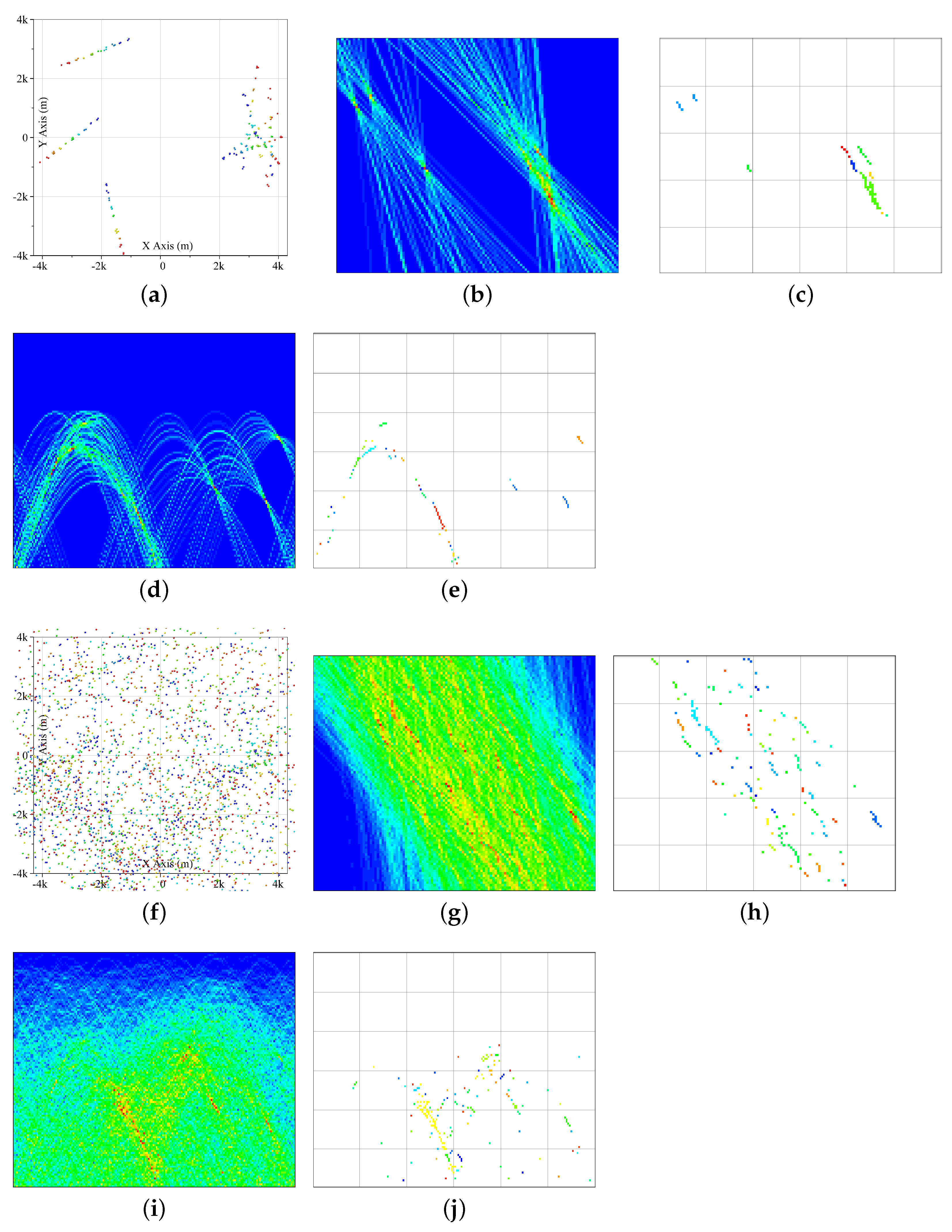
To access the superiority of the proposed method in TBD methods. Multi-dimensional HT-TBD [18] is performed with the synthetic data as comparison. The result is presented in Figure 6. In processing the 4D points with the method in [18], 2D HT is performed $\frac{4\times 3}{2}$ times by independently mapping each of the measured parameters versus the other three. Then, the most-likely linear target tracks for each data cluster are determined. After that, the candidate linear target tracks are associated. Finally, the intersections of the sets for the 6 HT domains are regarded as possible target tracks. The experiment of [18] consists of two parts, testing the multi-dimensional HT-TBD [18] method only using the target points and using the both the target points and clutter points. The multi-dimensional HT-TBD [18] is performed using the information of the X-axis and Y-axis.

Firstly, only the target points in Figure 6a are fed to the multi-dimensional HT-TBD. The parameter map in Figure 6b can be obtained if the gradient $k_p$ and intercept $b_p$ in (45) are the two parameters of the voting map.

$$\begin{array}{c}\hfill y_i=k_p\times x_i+b_p\end{array}$$

(45)

The widths of the gradient bin and intercept bin are 25 and 100, respectively. In (45), the $y_i$ and $x_i$ are the position on the X axis and timestamp, respectively. Figure 6b infers that the vote of the 3 individual tracks is outstanding compared with their surrounding cells. However, the vote of the close tracks, group 1 in Figure 5a, is overlapped. It is hard to distinguish the individual tracks. The cluster result of Figure 6b is presented in Figure 6c. The three individual tracks can be detected as three individual regions, and each region generates a candidate point set. It means the three tracks can be detected individually. However, the close tracks will be detected as one larger region, and the points of all 6 tracks in group 1 will be put in one set.

Then, another parameter space, range $\rho$ and azimuth $\theta$, is tested. The range $\rho$ and azimuth $\theta$ in (46) are constants if the target points in a straight line.

$$\begin{array}{c}\hfill \rho =x_i\times cos\left(\theta \right)+y_i\times sin\left(\theta \right)\end{array}$$

(46)

The widths of the range bin and azimuth bin are 100 m and $\pi /90$, respectively. In (46), the $y_i$ and $x_i$ are the position on the X axis and timestamp, respectively. The 2D HT map and corresponding result using the $\rho$ and $\theta$ are presented in Figure 6d,e. A similar problem arises in the close tracks. Figure 6c,e infers that the multi-dimensional HT-TBD [18] is available to detect individual targets but insufficient to detect close tracks.

Secondly, both the points of the target and clutter are processed by the multi-dimensional HT-TBD; the fed points are presented in Figure 6f. The result corresponding to (45) is presented in Figure 6g,h. The vote of targets is falling in that of enormous clutter. The correct candidate point set is missed. The result corresponding to (46) is presented in Figure 6i,j. The problem is similar. The result in Figure 6f–g infers that, in 4D scenarios, the multi-dimensional HT-TBD is insufficient to cope with the strong clutter backgrounds and clutter regions.

4.2. Real Data Experiment

To further access the performance of the proposed method. An extensive experiment using a 3D radar is performed. The coverage range of the radar is about 30 km, and the horizontal rotate speed of the radar antenna is $\pi$ rad/s, i.e., $t_{\mathrm{In}}=2$. The scope of the vertical angle for the elevation of targets is 0 to $\frac{\pi }{3}$. The targets in the surveillance area are multiple maneuvering airplanes. The GPS in the airplane records the ground truth of the airplane’s trajectory. The experiment contains two real scenarios. However, in both experiments, only the ground truth of the airplane which belongs to our experiment is available.

4.2.1. Experiment 1

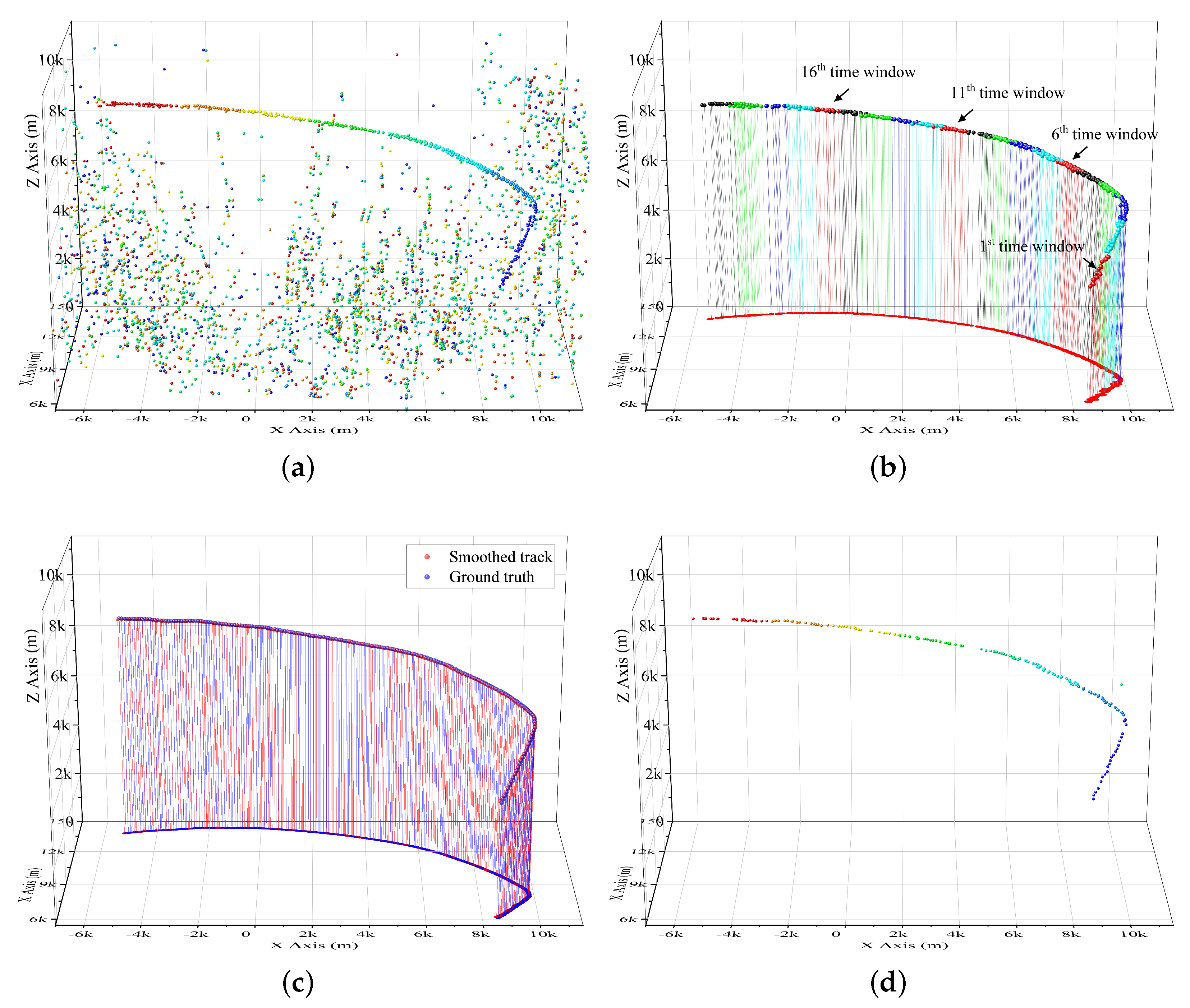
The measurements of scenario 1 are the unlabelled points presented in Figure 7a. It contains the measurements of 400 s, i.e., all the points from the $1\mathrm{st}$ to $200\mathrm{th}$ scan. The 3 axes of the figure regard the X position, Y position, and altitude. The point color regards the time information, the blue to red points denote the initial points to the most recently obtained points. The points are partitioned into time windows [21] to access the tracklet detection performance, and the points in each time window are individually processed. The width of the time window here is 20 s, i.e., the points of 10 scans are jointly processed.

The detected tracks in each time window are presented in Figure 7b. The target track can be well detected in each time window despite the inhomogeneous clutter background. It is worth noting that in the $3\mathrm{rd}$ and $4\mathrm{th}$ time windows, the target is maneuvering. Both the target course and speed are varying along with the time. The track is detected in $3\mathrm{rd}$ and $4\mathrm{th}$ time windows and infers that, although the method is designed for targets in a straight line, maneuvering targets can be also detected. The smoothed track can be obtained with the tracklet association method in [21]. The smoothed track is presented by the red line in Figure 7c. It matches well with the ground truth. Meanwhile, the PHD filter [35] in the 3D version is also tested, and the tracking result is presented in Figure 7d. An outline of the track can be obtained, but the target is lost in some scans. Meanwhile, in some scans, plenty of measurements (several times of measurement rate) are generated by the target. One target may be falsely detected as two close targets. So, some false alarm tracks are caused by the instability of the measurement rate.

Then, track smoothing and outlier removal are performed to decrease the position error of the track. The difference between the ground truth and the smoothed tracks is presented in Figure 8a. The red, blue, and green lines mean the difference in 3D space. In the $30\mathrm{th}$ to $40\mathrm{th}$ scan where the target is maneuvering, the difference is similar with the others. Those of the PHD filter [35] are presented in Figure 8b, and only the positional error of detected target is presented. Comparison between Figure 8a,b infers that the positional error of the two methods is similar. However, the positional error of scans where the target is maneuvering ($30\mathrm{th}$ to $40\mathrm{th}$ scan) is slightly larger than the other scans. In Figure 8c, the innovation square which evaluates the difference between the measurement and corresponding prediction is presented. In most scans, even the scans in which the target is maneuvering, the innovation of the method is stable and similar with the others. It means that our tracking method is stable to access the correct measurement point and to get a suitable prediction even if the target is maneuvering. Figure 8d shows the OSPA distance of methods [35,36,37,38] among 200 scans. The cut-off value and the distance order are 200 m and 1, respectively. The result of the real experiment, on average, is summarized in

Table 5. Result of two real experiments.

		Detection Rate	False Alarm Track	Detection vs. False Alarm	Positional Error	OSPA Distance
Experiment 1	Proposed method	100%	0	∞	70.88	70.88
	ET-PHD [35]	75.49%	0.1618	466.56%	96.69	92.92
	CPHD [36]	83.82%	0.7206	116.32%	88.63	124.04
	Bernoulli filter [37]	86.21%	0.5833	147.80%	70.41	108.31
	GLMB [38]	85.29%	0.6470	131.82%	68.91	110.77
Experiment 2	Proposed method	100%	0	∞	73.34	73.34
	ET-PHD [35]	75.34%	0.2422	311.06%	56.69	92.71
	CPHD [36]	85.29%	0.6471	131.82%	68.91	110.77
	Bernoulli filter [37]	84.09%	0.9182	91.58%	74.13	121.04
	GLMB [38]	81.36%	0.6909	117.76%	64.06	112.89

. The comparison infers that the ET-PHD filter [35] and the methods [36,37,38] are no better than the proposed method mainly because of the misdetection and false alarm track, respectively. We think it is an acceptable result to track a moving target whose speed is about 200 m per second.

4.2.2. Experiment 2

In the second experiment, the surveillance area has 2 tracks to access the tracking performance of close targets. The measurement of 220 scans is presented in Figure 9a. The longer track exists in all 220 scans, and the shorter one keeps 40 scans, from $151\mathrm{th}$ to $190\mathrm{th}$ scans. The two tracks are close with each other in $166\mathrm{th}$ to $180\mathrm{th}$ scans. Meanwhile, the clutter density in the region of track crossing is much larger than that of other regions. The 220 scans are partitioned into 22 not overlapped time windows. The tracks obtained in each time window are presented in Figure 9b. In the $15\mathrm{th}$ to $18\mathrm{th}$ time window, two tracks are obtained without false alarm tracks, even if the clutter region exists.

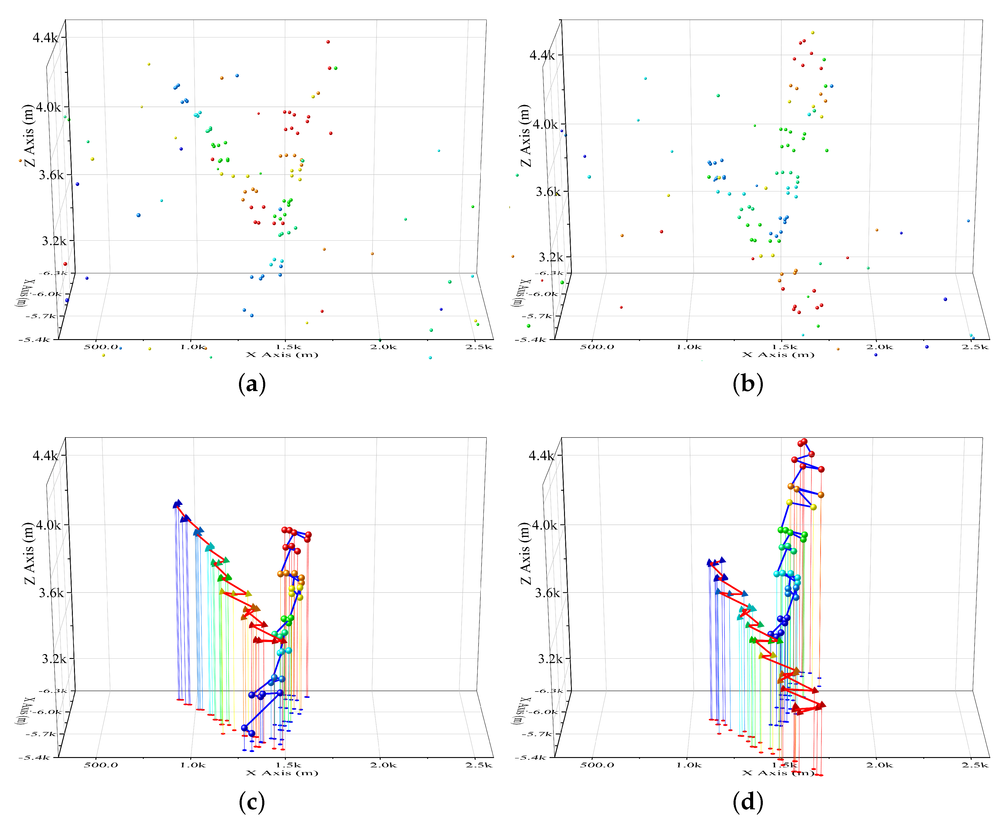
The points of $166\mathrm{th}$ to $175\mathrm{th}$ are presented in Figure 10a, and $171\mathrm{th}$ to $180\mathrm{th}$ are presented in Figure 10b. Among the 36 points of track 1, it has 12 points whose distance from the points of track 2 is smaller than 350 m. Among the 36 points of track 2, 11 points have a distance from track 1 smaller than 350 m. The nearest distance between two tracks is merely 268 m. The obtained track using the the points of Figure 10a is presented in Figure 10c. The obtained track in Figure 10b is presented in Figure 10d. The two tracks obtained are labeled by balls and triangles, respectively. Figure 10 infers that the points of closely distributed tracks can be well partitioned into correct tracks.

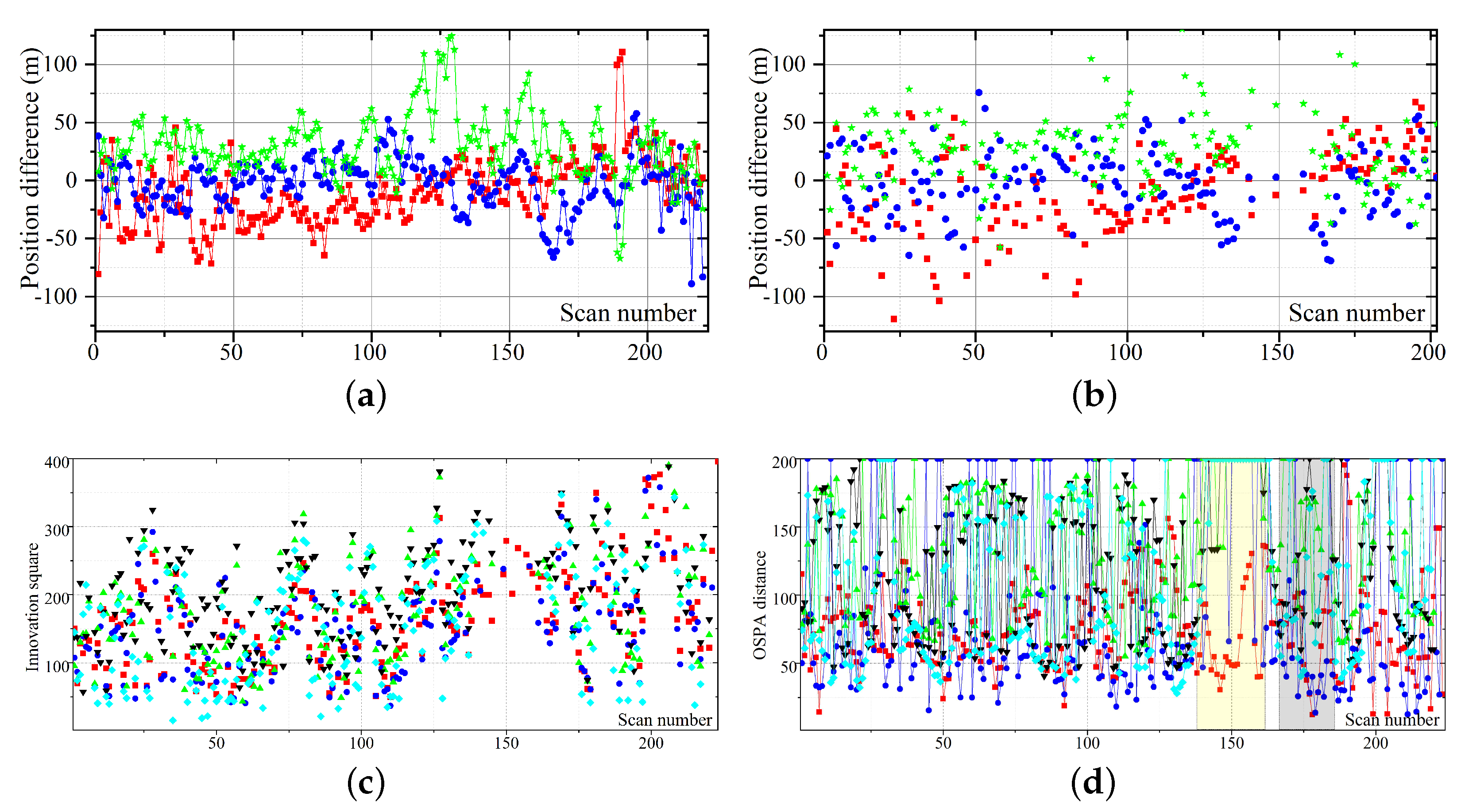
As to the position error, only the ground truth of track 1 is available. The position differences between the smoothed track and ground truth in X, Y, and Z axes using the proposed method are presented in Figure 11a. That of the ET-PHD filter is presented in Figure 11b. It infers that lots of false alarm tracks are built by the clutter region. Meanwhile, the target is lost in 22 successive scans for the clutter region. In Figure 8c, the innovation square of the five methods is presented, which proves the stability of the proposed method in multiple target tracking. The overall OSPA distance of 220 scans is presented in Figure 11d. In Figure 11d, the gray rectangle labels the scans in which two tracks are close with each other. It infers that the corresponding position error is similar to the other scans. The yellow rectangle labels the scans, $140\mathrm{th}$ to $160\mathrm{th}$, in which the target is quite weak and merely generates a few measurements per scan. It has 3.21 target points per scan, on average, in all 220 scans and 1.39 target points during $140\mathrm{th}$ to $160\mathrm{th}$ scans. The target is hard to detect in these scans by using the comparisons [35,36,37,38]. The result further proves that the proposed method works well in close track scenarios.

The result summarized in Table 5 infers that the proposed method is superior in suppression of clutter region and detection of a weak target for the benefit of multi-scan detection.

5. Conclusions

In this work, a 4D TBD is developed for extended target detection in 3D radar systems. The problem is designed to detect the closely distributed weak extended targets using the 3D positional information and timestamp of points, in spite of heterogeneous background clutter and various clutter regions. The method is divided into three parts, and plenty of detection bins are built. The 4D TBD process is completed by a 3D TBD and three 2D TBD. Although the proposed 4D TBD is designed for the straight-line targets, the experiment using the real data infers that the method also works well for closely maneuvering targets.

References

1. Jevtic, M.; Markovic, K.; Mikluc, D.; Misic, B.; Pajic, T.T. Real-time implementation of target tracking system for air surveillance radar applications. In Proceedings of the 11th International Conference on Telecommunication in Modern Satellite, Cable and Broadcasting Services (TELSIKS), Nis, Serbia, 16–19 October 2013; Volume 10. [Google Scholar]
2. Yan, B.; Xu, N.; Zhao, W.-B.; Xu, L.-P. A Three-Dimensional Hough Transform-Based Track-Before-Detect Technique for Detecting Extended Targets in Strong Clutter Backgrounds. Sensors 2019, 19, 881. [Google Scholar] [CrossRef] [Green Version]
3. Granström, K.; Natale, A.; Braca, P.; Ludeno, G.; Serafino, F. Gamma Gaussian inverse Wishart probability hypothesis density for extended target tracking using X-band marine radar data. IEEE Trans. Geosci. Remote Sens. 2015, 53, 6617–6631. [Google Scholar] [CrossRef]
4. Orguner, U.; Lundquist, C.; Granström, K. Extended target tracking with a cardinalized probability hypothesis density filter. In Proceedings of the 14th International Conference on Information Fusion, Milan, Italy, 3–6 June 2011; pp. 1–8. [Google Scholar]
5. Yan, B.; Xu, N.; Xu, L.P.; Mu, Q.; Cheng, P. An improved partitioning algorithm based on FCM algorithm for extended target tracking in PHD filter. Digit. Signal Process. 2019, 90, 54–70. [Google Scholar] [CrossRef]
6. Orlando, D.; Ehlers, F.; Ricci, G. Track-before-detect algorithms for bistatic sonars. In Proceedings of the 2010 2nd International Workshop on Cognitive Information Processing, Elba, Italy, 14–16 June 2010; pp. 180–185. [Google Scholar]
7. Ehlers, F.; Orlando, D.; Ricci, G. Batch tracking algorithm for multistatic sonars. IET Radar Sonar Navig. 2012, 6, 746–752. [Google Scholar] [CrossRef]
8. Orlando, D.; Venturino, L.; Lops, M.; Ricci, G. Track-Before-Detect Strategies for STAP Radars. IEEE Trans. Signal Process. 2010, 58, 933–938. [Google Scholar] [CrossRef]
9. Yi, W.; Morelande, M.R.; Kong, L.; Yang, J. An Efficient Multi-Frame Track-Before-Detect Algorithm for Multi-Target Tracking. IEEE Sel. Top. Signal Process. 2013, 7, 421–434. [Google Scholar] [CrossRef]
10. Yan, B.; Xu, L.; Li, M.; Yan, J.Z. Track-before-detect algorithm based on dynamic programming for multi-extended-targets detection. IET Signal Process. 2017, 11, 674–686. [Google Scholar] [CrossRef]
11. Yi, W.; Fang, Z.; Li, W.; Hoseinnezhad, R.; Kong, L. Multi-Frame Track-Before-Detect Algorithm for Maneuvering Target Tracking. IEEE Trans. Veh. Technol. 2020, 69, 4104–4118. [Google Scholar] [CrossRef]
12. Garcia-Fernandez, A.F. Track-before-detect labeled multi-bernoulli particle filter with label switching. IEEE Trans. Aerosp. Electron. Syst. 2016, 52, 2123–2138. [Google Scholar] [CrossRef]
13. Garcia-Fernandez, A.F. Track before detect for radar using stochastic particle flow filters. In Proceedings of the 2020 IEEE Radar Conference (RadarConf20), Florence, Italy, 21–25 September 2020; pp. 1–6. [Google Scholar]
14. Bao, Z.; Jiang, Q.; Liu, F. A PHD-Based Particle Filter for Detecting and Tracking Multiple Weak Targets. IEEE Access 2019, 7, 145843–145850. [Google Scholar] [CrossRef]
15. Zhichao, B.; Qiuxi, J.; Fangzheng, L. Multiple model efficient particle filter based track-before-detect for maneuvering weak targets. J. Syst. Eng. Electron. 2020, 31, 647–656. [Google Scholar] [CrossRef]
16. Kim, D.; Ristic, B.; Guan, R.; Rosenberg, L. A Bernoulli Track-Before-Detect Filter for Interacting Targets in Maritime Radar. IEEE Trans. Aerosp. Electron. Syst. 2021, 57, 1981–1991. [Google Scholar] [CrossRef]
17. Carlson, B.D.; Evans, E.D.; Wilson, S.L. Search radar detection and track with the Hough transform. I. system concept Track-Before-Detect Filter for Interacting Targets in Maritime Radar. IEEE Trans. Aerosp. Electron. Syst. 1994, 30, 102–108. [Google Scholar] [CrossRef]
18. Moyer, L.R.; Spak, J.; Lamanna, P. A Multi-Dimensional Hough Transform-Based Track-Before-Detect Technique for Detecting Weak Targets in Strong Clutter Backgrounds. IEEE Trans. Aerosp. Electron. Syst. 2011, 47, 3062–3068. [Google Scholar] [CrossRef]
19. Yan, B.; Xu, N.; Wang, G.; Yang, S.; Xu, L.P. Detection of Multiple Maneuvering Extended Targets by Three-Dimensional Hough Transform and Multiple Hypothesis Tracking. IEEE Access 2019, 7, 80717–80732. [Google Scholar] [CrossRef]
20. Yan, B.; Zhao, X.Y.; Xu, N.; Chen, Y.; Zhao, W.B. A grey wolf optimization-based track-before-detect method for maneuvering extended target detection and tracking. Sensors 2019, 19, 1577. [Google Scholar] [CrossRef] [PubMed] [Green Version]
21. Yan, B.; Enrico, P.; Xu, N.; Sun, Z.; Xu, L.P. Multiple Maneuvering Extended Targets Detection by 3D Projection and Tracklet Association. Signal Process. 2021, 179, 107821. [Google Scholar] [CrossRef]
22. Fiscante, N.; Addabbo, P.; Clemente, C.; Biondi, F.; Giunta, G.; Orlando, D. A Track-Before-Detect Strategy Based on Sparse Data Processing for Air Surveillance Radar Applications. Remote Sens. 2021, 13, 662. [Google Scholar] [CrossRef]
23. Peng, D.; Jing, Z.; Gong, D.; Tang, B. Maneuvering multi-target tracking based on variable structure multiple model GMCPHD filter. Signal Process. 2017, 141, 158–167. [Google Scholar]
24. Liu, Z.; Wei, X.; Li, X. Adaptive clutter suppression for airborne random pulse repetition interval radar based on compressed sensing. Prog. Electromagn. Res. 2012, 128, 291–311. [Google Scholar] [CrossRef] [Green Version]
25. Benavoli, A.; Chisci, L.; Farina, A.; Immediata, S.; Timmoneri, L.; Zappa, G. Knowledge-based system for multi-target tracking in a littoral environment. IEEE Trans. Aerosp. Electron. Syst. 2006, 42, 1100–1119. [Google Scholar] [CrossRef] [Green Version]
26. Yan, B.; Xu, N.; Zhao, W.; Li, M.; Xu, L. An Efficient Extended Targets Detection Framework Based on Sampling and Spatio-Temporal Detection. Sensors 2019, 19, 2912. [Google Scholar] [CrossRef] [PubMed] [Green Version]
27. Musicki, D.; Suvorova, S.; Morelande, M.; Moran, B. Clutter map and target tracking. In Proceedings of the 7th International Conference on Information Fusion, Philadelphia, PA, USA, 25–28 July 2005; Volume 1, pp. 1–8. [Google Scholar]
28. Zhou, G.; Yu, C.; Zong, C.; Quan, T.; Cui, N. Clutter-knowledge-based target tracking method in complex conditions. IET Int. Radar Conf. 2009, 1, 1–5. [Google Scholar]
29. Chen, X.; Tharmarasa, R.; Pelletier, M.; Kirubarajan, T. Integrated Bayesian clutter estimation with JIPDA/MHT trackers. IEEE Trans. Aerosp. Electron. Syst. 2013, 49, 395–414. [Google Scholar] [CrossRef]
30. Chen, X.; Tharmarasa, R.; Kirubarajan, T.; McDonald, M. Online clutter estimation using a Gaussian kernel density estimator for multitarget tracking. IET Radar Sonar Navig. 2015, 9, 1–9. [Google Scholar] [CrossRef]
31. Sobhani, B.; Zwick, T.; Chiani, M. Target TOA association with the hough transform in UWB radars. IEEE Trans. Aerosp. Electron. Syst. 2016, 52, 743–754. [Google Scholar] [CrossRef]
32. Dalitz, C.; Schramke, T.; Jeltsch, M. Iterative Hough transform for line detection in 3D point clouds. Image Process. Line 2017, 7, 184–196. [Google Scholar] [CrossRef] [Green Version]
33. Yan, B.; Andrea, G.; Paolini, E. A Track-Before-Detect Approach for UWB Radar Sensor Networks. In Proceedings of the IEEE Radar Conference, Florence, Italy, 21–25 September 2020; pp. 1–6. [Google Scholar]
34. Yan, B.; Andrea, G.; Paolini, E. A Track-Before-Detect Algorithm for UWB Radar Sensor Networks. Signal Process. 2021, 5, 108257. [Google Scholar] [CrossRef]
35. Granstrom, K.; Lundquist, C.; Orguner, O. Extended target tracking using a Gaussian-mixture PHD filter. IEEE Trans. Aerosp. Electron. Syst. 2012, 48, 3268–3286. [Google Scholar] [CrossRef] [Green Version]
36. Vo, B.-N.; Vo, B.-T.; Cantoni, A. Analytic Implementations of the Cardinalized Probability Hypothesis Density Filter. IEEE Trans. Signal Process. 2007, 55, 3553–3567. [Google Scholar] [CrossRef]
37. Vo, B.-T.; See, C.M.; Ma, N.; Ng, W.T. Multi-Sensor Joint Detection and Tracking with the Bernoulli Filter. IEEE Trans. Aerosp. Electron. Syst. 2012, 48, 1385–1402. [Google Scholar] [CrossRef]
38. Vo, B.-N.; Vo, B.-T.; Hung, H. An Efficient Implementation of the Generalized Labeled Multi-Bernoulli Filter. IEEE Trans. Signal Process. 2017, 65, 1975–1987. [Google Scholar] [CrossRef] [Green Version]
Figure 1. The flowchart of the proposed method.
Remotesensing 13 04942 g001
Figure 2. The flowchart of the proposed method.
Remotesensing 13 04942 g002
Figure 3. The 2D Hough transformation on three axes.
Remotesensing 13 04942 g003
Figure 4. (a) Simulation for T d , opt 1 . (b) Simulation for T d , opt 2 .
Remotesensing 13 04942 g004
Figure 5. (a) The simulation scenario. (b) The measurements in one experiment. (c) The target points obtained from 200 Monte Carlo experiments (before trajectory smoothing).
Remotesensing 13 04942 g005
Figure 6. (a) Target points in 2D version. (b) Parameter map of 2D HT using (45) and only using target points. (c) Cluster result of 2D HT parameter map using (45). (d) Parameter map of 2D HT using (46) and only using target points. (e) Cluster result of 2D HT parameter map using (46). (f) All measurement points in 2D version. (g) Parameter map of 2D HT using (45) and using all measurements. (h) Cluster result of 2D HT parameter map using (45). (i) Parameter map of 2D HT using (46) and using all measurements. (j) Cluster result of 2DHT parameter map using (46).
Remotesensing 13 04942 g006
Figure 7. (a) The measurements in of scenario 1 among 1 to 200 scans. (b) The tracklets obtained in 20 time windows. (c) The smoothed track and the ground truth. (d) The target position obtained by the ET-PHD filter [35].
Remotesensing 13 04942 g007
Figure 8. (a) The position difference between the smoothed track and ground truth of X, Y, and Z axes using the proposed method. (b) The position difference between the smoothed track and ground truth of X, Y, and Z axes using the ET-PHD filter [35]. (c) The innovation square of the proposed method and four comparisons [35,36,37,38]. (d) The OSPA distance of the proposed method and four comparisons [35,36,37,38]. In (c,d), red squares mean the proposed method, blue balls mean the ET-PHD [35], green triangles mean the CPHD filter [36], black inverted triangles mean the Bernoulli filter [37], and cyan diamonds mean the GLMB filter [38].
Remotesensing 13 04942 g008
Figure 9. (a) The measurements in scenario 2 among 1 to 220 scans. (b) The tracklets obtained in 22 time windows. (c) The smoothed track and the ground truth. (d) The target position obtained by the ET-PHD filter [35].
Remotesensing 13 04942 g009
Figure 10. (a) The measurement of 166th to 175th scans. (b) The measurement of 171th to 180th scans. (c) The two obtained tracks corresponding to Figure 10a. (d) The two obtained tracks corresponding to Figure 10b.
Remotesensing 13 04942 g010
Figure 11. (a) The position difference between the smoothed track and ground truth of X, Y, and Z axes using the proposed method. (b) The position difference between the smoothed track and ground truth of X, Y, and Z axes using the ET-PHD filter [35]. (c) The innovation square of the proposed method and four comparisons [35,36,37,38]. (d) The OSPA distance of the proposed method and four comparisons [35,36,37,38]. Yellow rectangle means weak target scans. Gray rectangle means closely targeted scans. In (c,d), red squares mean the proposed method, blue balls mean the ET-PHD [35], green triangles mean the CPHD filter [36], black inverted triangles mean the Bernoulli filter [37], and cyan diamonds mean the GLMB filter [38].
Remotesensing 13 04942 g011