Article

An Improved Smooth Variable Structure Filter for Robust Target Tracking

1
School of Aerospace Science and Technology, Xidian University, Xi’an 710126, China
2
Department of Electrical, Electronic, and Information Engineering, University of Bologna, 47521 Cesena (FC), Italy
*
Author to whom correspondence should be addressed.
Remote Sens. 2021, 13(22), 4612; https://doi.org/10.3390/rs13224612
Submission received: 20 August 2021 / Revised: 11 November 2021 / Accepted: 12 November 2021 / Published: 16 November 2021
(This article belongs to the Special Issue Radar Signal Processing for Target Tracking)

Abstract

:
As a new-style filter, the smooth variable structure filter (SVSF) has attracted significant interest. Based on the predictor-corrector method and sliding mode concept, the SVSF is more robust in the face of modeling errors and uncertainties compared to the Kalman filter. Since the estimation performance is usually insufficient in real cases where the measurement vector is of fewer dimensions than the state vector, an improved SVSF (ISVSF) is proposed by combining the existing SVSF with Bayesian theory. The ISVSF contains two steps: firstly, a preliminary estimation is performed by SVSF. Secondly, Bayesian formulas are adopted to improve the estimation for higher accuracy. The ISVSF shows high robustness in dealing with modeling uncertainties and noise. It is noticeable that ISVSF could deliver satisfying performance even if the state of the system is undergoing a sudden change. According to the simulation results of target tracking, the proposed ISVSF performance can be better than that obtained with existing filters.

1. Introduction

State estimation of dynamic systems has been widely used in various engineering fields, such as target tracking, navigation, signal processing, computer vision, automatic control, etc. [1,2]. However, a variety of noise and interference have made systems more complex and changeable. This makes accurate information about noise statistics and system models not readily available. Besides that, the system state may have a sudden change, which means that when a state encounters unknown external interference, it may change suddenly and dramatically in forms similar to the sinusoid wave and rectangular wave. As a result, efforts to develop new methods to improve system robustness and estimation accuracy have been under active consideration recently.
Various filters have been developed to estimate the system state value according to the measurements. The Kalman filter (KF) [3], the most widely used filter in linear Gaussian systems, is the optimal method under the criteria of minimum mean square error, maximum likelihood and maximum posterior. However, in nonlinear systems, the KF may be affected by divergence. So, a variety of filters have been developed for better estimation performance in a nonlinear system, which mainly can be divided into three categories. In the first category, the nonlinear system is simplified into a linear one. A typical example in this category is the extended Kalman filter (EKF) [4,5], in which the nonlinear system is simplified as a linear one by only utilizing the first-order Taylor expansion and discarding the higher-order terms. In the second category, the probability density distribution of a nonlinear function is replaced by selecting a certain number of sigma points, and the posterior probability density are calculated by these points. These methods have been termed “numerical integration methods” [6]. The two most widely used methods of this category are the unscented Kalman filter (UKF) and the cubature Kalman filter (CKF) [7]. The last category is based on particle filter methods, which work well in nonlinear and non-Gaussian systems but are time-consuming in iterative computation [8,9]. Given that, the particle filters may not meet the time requirement in some real cases. Some cutting-edge methods such as the generalized regression neural network have also been applied in target tracking [10,11].
Knowledge of the mathematical model and noise statistics is essential in a majority of existing methods, and the robustness of these methods would be severely reduced if inappropriate modeling or noise modeling are used. Therefore, filters of higher robustness have been proposed to deal with uncertainties of models and noise. For example, one of the most widely used methods in handling model uncertainty is an adaptive strategy using “multiple models” based on the Bayesian framework. Additionally, the strategy usually implements the interactive multi-model method [1] or the variable structure interactive multi-model [12]. In real cases, various noises need to be reduced, such as the heavy-tailed noise [13], non-Gaussian distributions noise [14] and Student’s t distribution noise [15]. The combination of noise models and the adaptive methods in [13,14,15] have achieved good results. However, all of the mentioned algorithms are built on the Kalman filter, and thus, some shortcomings still exist, such as sensitivity to parameters, etc. In order to improve the robustness of the filter in terms of model uncertainties and anti-noise interference ability, the smooth variable structure filter (SVSF) has been developed [16].
The SVSF [16] is a recently developed filter that is designed to handle the issue of model uncertainty and noise interference. The estimated state of the SVSF is constrained to fluctuate around the true state trajectory within a small region and shows high robustness and stability. The SVSF is simple in structure and feasible to implement. However, it is regarded as a suboptimal filter [7,17] due to its low accuracy. Therefore, [18] attempts have been made to refine the SVSF by deducing the its state error covariance. They show that the priori and posteriori state error covariance matrices of the SVSF are similar to the KF in linear systems, and are expected to extend to other applications. The authors of [19] further deduced the optimal bounded layer width of SVSF based on the posterior state covariance matrix. Based on this, the SVSF is combined with other filters (such as KF, EKF, UKF, and CKF), which can take advantage of both the robustness of the SVSF and the accuracy of these filters [7,17,20,21]. For example, combinations of SVSF with the UKF (UK-SVSF) or CKF (CK-SVSF) filtering systems [20] are better than separate methods, but will be affected by their own disadvantages and interference with each other. In [22], the dependence of the estimation performance on parameters is avoided by an uncertainty learning strategy. Additionally, the second-order SVSF [23] and other methods [20,24] have been proposed to improve the stability and robustness. Since its development, the SVSF has been applied in various applications [25], such as vehicle navigation [24,26,27,28,29,30,31], fault detection and diagnosis [32,33], battery management [34,35,36,37], and artificial intelligence [33,38,39]. However, it was found that the SVSF can be further improved if two shortcomings can be solved. (1) The SVSF is generally used in systems with one measurement corresponding to each state variable. When the dimension of the measurement vector is less than that of the state variables, the original SVSF cannot estimate the lower partition of the state vector. For example, tracking sensors usually measure the target position but do not record the velocity and acceleration of the target. Thus, [16] developed a similar Luenberger’s reduced order observer strategy, which constructs a reduced order estimator to estimate the lower partition of the state vector. However, the system is required to be completely observable and completely controllable, and meanwhile, the calculation process for the lower partition of the state vector needs to be independent, which greatly limits the versatility of the method. Another popular solution [17,21] is to construct an “artificial” measurement of the lower partition of the state vector, which is portable and widely used. However, the estimation of the lower partition of the state vector cannot achieve satisfactory results when the measurement noise intensity is high. (2) In short, compared with filters based on Bayesian theory, the SVSF is insufficient to suppress noise. If the noise can be further eliminated, the performance of the SVSF can be greatly improved and the SVSF could be advantageous in more applications.
An improved smooth variable structure filter (ISVSF), devoted to solving the above described shortcomings, is proposed here. It is built on the basis of the SVSF and inspired by the Bayesian theory [40]. In line with the SVSF strategy, the proposed ISVSF deduces the priori and posterior error covariance matrix of the state variables in the linear system. The Bayesian method is exploited to calculate the new state estimation by means of estimated state and error covariance of SVSF.
Three main advantages of the ISVSF are as follows. (1) The ISVSF can maintain high robustness even if the system state is undergoing sudden change or the modeling is deviating from the actual model. (2) Compared with the original SVSF, the exploited Bayesian method contributes to a higher estimation accuracy. Meanwhile, the obtained error covariance matrix is helpful in further improving application with other methods, such as the interacting multiple model methods or constructing smoother. (3) When the dimension of the state variables is larger than that of the measurements, the state error covariance will be exploited to estimate the lower partition of the state vector in ISVSF. ISVSF is a newer strategy than the previous method [16,17] of the SVSF system, and it has computational complexity almost identical to that of the Kalman filter.
In general, this paper proposes the real-time ISVSF as it could achieve the high accuracy of the Bayesian solution and robustness similar to that of the SVSF. The ISVSF proposed here also can be applied in systems with states undergoing sudden changes. However, our former work [41] proposed a non real-time smoother, which is also applied in maneuvering target tracking. The rest of the paper is structured as follows: The review of the SVSF will be presented in Section 2, the elaborate explanation of the proposed ISVSF algorithm in Section 3, the simulation process and an analysis in Section 4 and conclusions of the main findings in this paper in Section 5. Table 1 provides a list of nomenclature used throughout the paper.

2. The SVSF Strategies

2.1. The SVSF

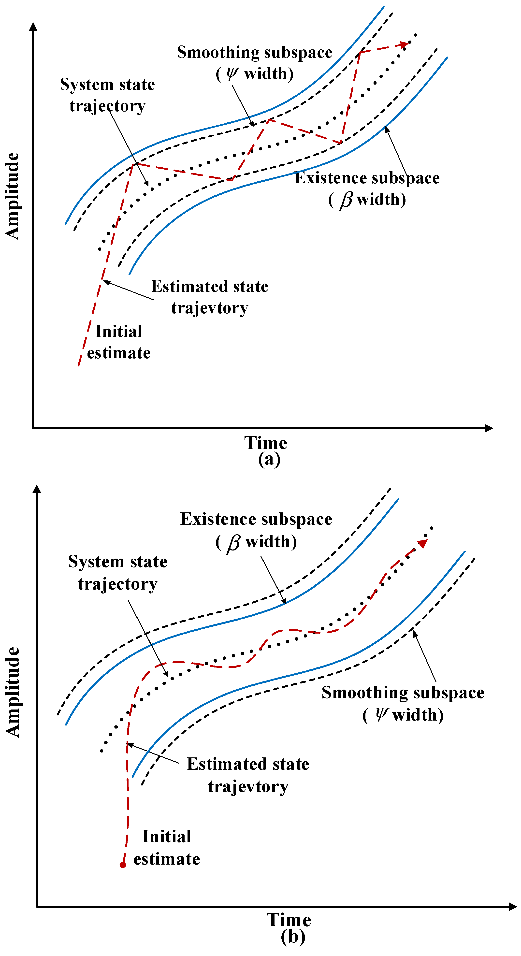
In 2003, Habibi and Burton proposed a novel form of predictor-corrector filter, called the variable structure filter (VSF) [42]. The VSF uses sliding mode concepts to construct a switching gain, which makes the state estimates converge within a boundary of the real value to ensure system stability. Based on the VSF, the SVSF was proposed with a less complex gain in 2007 [16]. As shown in Figure 1, the true trajectory of the system has some fluctuations caused by dynamic interference or disturbance noises. The estimated state trajectory gradually approaches the real trajectory until it reaches the existence subspace. If it remains in the existence subspace, the estimated state is forced to switch back and forth on the real state trajectory by SVSF gain [24]. If the errors caused by modeling error and noise are bounded, then the state estimates will be kept within a limit. The SVSF strategy ensures stability and robustness in resolving modeling uncertainties and errors.
In the case of linear dynamic systems under a zero-mean and Gaussian noise, the state equation and observation equation of a dynamic system are as follows:
{ x k + 1 = F x k + w k z k + 1 = H x k + 1 + v k + 1
where k is the discrete time, x k n is the state vector, and F n × n is the system model matrix or the state transition matrix. z k m is the measurement, H m × n is the linear measurement (out) matrix, w k n and v k m are the process noise vector and the measurement noise, respectively, and their covariances are represented by R k and Q k , respectively.
The iterative process of SVSF contains two steps and can be summarized as follows:
The prediction stage: the predicted state estimate x ^ k + 1 | k is calculated according to the system model matrix F and the previous state estimate x ^ k | k .
x ^ k + 1 | k = F x ^ k | k
A priori estimated measurement z ^ k + 1 | k is calculated according to the priori estimated state x ^ k + 1 | k and the measurement matrix H is as follows:
z ^ k + 1 | k = H x ^ k + 1 | k
The priori measurement innovations e k + 1 | k svsf are calculated in SVSF as:
e k + 1 | k svsf = z k + 1 z ^ k + 1 | k
The updating stage: the SVSF’s corrective gain K k + 1 svsf [16] is calculated as follows:
K k + 1 svsf = H + diag [ ( | e k + 1 svsf | + γ | e k | k | ) sat ( ψ ¯ 1 e k + 1 svsf ) ] [ diag ( e k + 1 svsf ) ] 1
where K k + 1 svsf is a gain function, H + is the pseudoinverse matrix of H , and the diag function is to construct diagonal matrix. | e | is the absolute value of e , γ ( 0 γ < 1 ) is the SVSF’s “memory” (convergence rate), and represents the Hadamard product. s a t is a saturation function. Besides that,
sat ( ψ ¯ 1 e k + 1 | k svsf ) = { 1 , ψ ¯ 1 e k + 1 | k svsf 1 ψ ¯ 1 e k + 1 | k svsf , 1 < ψ ¯ 1 e k + 1 | k svsf < 1 1 , ψ ¯ 1 e k + 1 | k svsf 1
and
ψ ¯ 1 = [ 1 ψ 1 0 0 0 0 0 0 1 ψ m ]
where ψ i ( i = 1 m ) represents the width of the smoothing boundary layer in every dimension, the value setting is described in [16,19], and m is the dimension of state estimation. The estimated state x ^ k + 1 | k + 1 is updated as follows:
x ^ k + 1 | k + 1 = x ^ k + 1 | k + K k + 1 | k svsf e k + 1 | k svsf
The posterior measurement estimate z ^ k + 1 | k + 1 and its innovation e k + 1 | k + 1 are described as:
z ^ k + 1 | k + 1 = H x ^ k + 1 | k + 1
e k + 1 | k + 1 = z k + 1 z ^ k + 1 | k + 1
The influence of existence subspaces on estimation is shown in Figure 2. The width of the existence subspace β is unknown and dynamic, and contains modeling errors and noises. Additionally, as indicated by [16], an upper bound can be selected according to a priori knowledge [17]. As shown in Figure 2, once the estimated state enters the existence subspace, the estimated state (by SVSF gain) will remain in the existence subspace and switch back and forth along the true state trajectory [17], and a high-frequency switching is called chattering [24]. The smoothing boundary layer ψ can decrease the chattering amplitude and make the estimated state trajectory smoother. The smoothing boundary layer ψ can reflect the level of interference and uncertainties. As shown in Figure 2a, when ψ β , the uncertain factors are underestimated [16] and the filter gain is more easily affected by the uncertain factors; therefore, the chattering appears. However, when the smoothing boundary layer is larger than the existence boundary layer ( ψ > β ), the chattering effects will be removed [24], as shown in Figure 2b.
SVSF is applied in systems where the state variables and measurement vector share the same dimension. Compared with the KF, SVSF has to rely on Luenberger’s strategy [16] or the “artificial” measurement [17] if measurements are less than states.

2.2. Review of Combining SVSF with Other Estimation Strategies

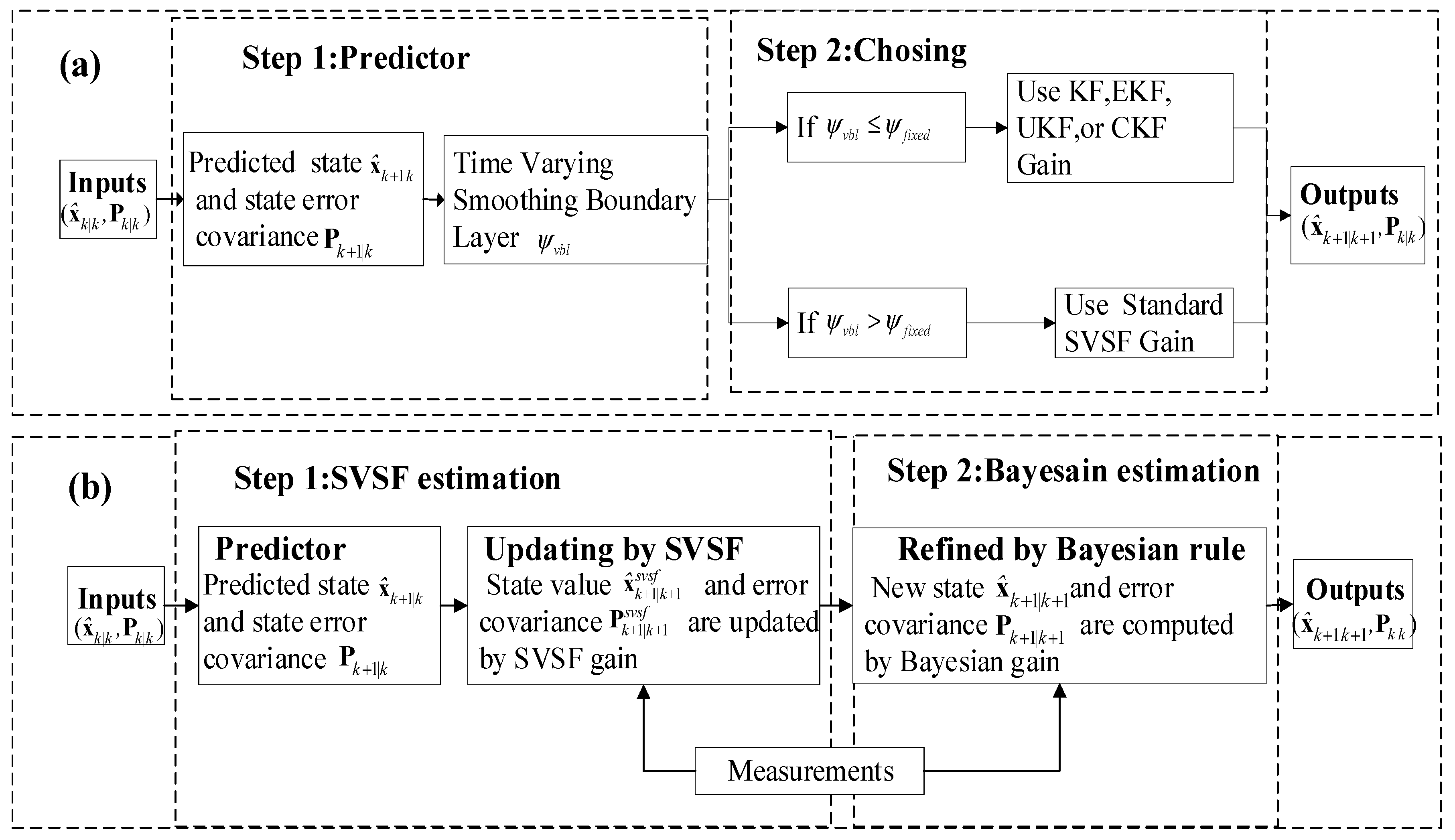
The development, improvement and application of the SVSF and its variants are discussed in the introduction [20]. Particularly, among the derivative methods of SVSF, the combination of the SVSF with different filtering is an effective solution to improve accuracy while preserving robustness even if model uncertainties exist [20]. To satisfy different demands, SVSF has been combined with EKF (EK-SVSF), UKF (UK-SVSF) and CKF (CK-SVSF). Those methods have the same structure, and the difference between SVSF and those combinations lies in the calculation of the gain as shown in Figure 3a. Given that, the calculated time varying smoothing boundary layer ψ vbl is compared with the fixed varying smoothing boundary layer ψ fixed to determine which gain will be utilized (e.g., SVSF or other filters); if ψ vbl ψ fixed ,the KF-based gain will be used to obtain optimality. If ψ vbl > ψ fixed , the standard SVSF gain is used to keep robustness at the cost of estimation accuracy.
The UK-SVSF is one of popular methods in the combination strategies and has been applied in many different systems [20,21,43,44]. For better understanding of the combination strategy, the UK-SVSF is chosen and its specific process is summarized as follows. The UKF uses the 2 n + 1 sigma points to estimate state. The sigma points and their corresponding weights are selected based on the following rules.
X 0 , k | k = x ^ k | k
W 0 = κ n + κ
where the X 0 , k | k is the first sigma point and W 0 is its corresponding weight, n is n -dimensional of state, κ is a design value (a small value less than 1 or that can be calculated by κ = 3 n ), and the next i = 1 , , n points and corresponding weights can be computed as:
X i , k | k = x ^ k | k + ( ( n + κ ) P k | k ) i
W i = 1 2 ( n + κ )
where ( ( n + κ ) P k | k ) i is the i - th column of the square root of ( n + κ ) P k | k , and W i is associated with the X i , k | k sigma points. The rest of the i = n + 1 , , 2 n points and their corresponding weights may be derived as:
X i , k | k = x ^ k | k ( ( n + κ ) P k | k ) i
W i = 1 2 ( n + κ )
The propagation of these sigma points can be calculated as:
X ^ i , k + 1 | k = f ( X ^ i , k | k )
The predicted state estimate and predicted state error covariance are calculated as follows:
x ^ k + 1 | k = i = 0 2 n W i X ^ i , k + 1 | k
P k + 1 | k = i = 0 i = 2 n W i ( X ^ i , k + 1 | k x ^ k + 1 | k ) ( X ^ i , k + 1 | k x ^ k + 1 | k ) T + Q k + 1
The nonlinear measurement propagation can be calculated as follows:
Z ^ i , k + 1 | k = h ( X ^ i , k + 1 | k )
where h is the measurement function. The predicted measurement z ^ k + 1 | k and the priori measurement innovation e k + 1 | k can be calculated as follows:
z ^ k + 1 | k = i = 0 2 n W i Z ^ i , k + 1 | k
e k + 1 | k = z k z ^ k + 1 | k
The predicted measurement covariance and the cross-covariance (between state and measurement) are calculated as follows:
P z z , k + 1 | k = i = 0 i = 2 n W i ( Z ^ i , k + 1 | k z ^ k + 1 | k ) ( Z ^ i , k + 1 | k z ^ k + 1 | k ) T + R k + 1
P x z , k + 1 | k = i = 0 i = 2 n W i ( X ^ i , k + 1 | k x ^ k + 1 | k ) ( Z ^ i , k + 1 | k z ^ k + 1 | k ) T
From (23) and (24), the UKF gain can be computed as follows:
K UKF , k + 1 = P x z , k + 1 | k P z z , k + 1 | k 1
The time varying boundary layer width is calculated as follows:
ψ vbl = ( A 1 H P k + 1 | k H T P z z , k + 1 | k 1 )
where
A = diag ( | e k + 1 | k | + γ | e k | k | )
If ψ vbl ψ fixed , the gain is updated by K k + 1 = K UKF , k + 1 , otherwise when ψ vbl > ψ fixed , K k + 1 = K k + 1 svsf is derived through the SVSF-based Equation (5). So, the state is updated as follows:
x ^ k + 1 | k + 1 = x ^ k + 1 | k + K k + 1 e k + 1 | k
Finally the covariance and the posteriori error are updated as follows:
P k + 1 | k + 1 = ( I K k + 1 H ) P k + 1 | k ( I K k + 1 H ) T + K k + 1 R k + 1 K k + 1 T
e k + 1 | k + 1 = z k + 1 h ( x ^ k + 1 | k + 1 )
However, those methods still have disadvantages. When the dimension of the measurement vector is less than that of the state variables, the original SVSF cannot estimate the lower partition of the state vector, and thus the accuracy will be decreased. If ψ vbl > ψ fixed appears frequently, the accuracy of the combination methods will decrease because the standard SVSF gain is used. However the proposed ISVSF can overcome this shortcoming.

3. Methodology for the Proposed ISVSF

3.1. Motivation of This Work

A generalized version of the SVSF cannot estimate the lower partition of the state vector when there are fewer dimensions of measurements than state, which can be overcome in Bayesian filters. This kind of filter, based on Bayesian theory, uses the state error covariance to obtain the probability density function and calculate the optimal gain to estimate the state value. Since the state error covariance can reflect a positive correlation among different dimensions of the state vector, even if the lower partition of the state vector has no corresponding measurements, it can still be precisely estimated. Inspired by this, the ISVSF was integrated with the Bayesian theory to estimate the lower partition of the state vector, which cannot been estimated in the SVSF.
Many practical algorithms based on the Bayesian filtering method are widely used, such as KF, EKF, UKF, PF, etc. From the Bayesian viewpoint, the estimation is to recursively calculate a certain degree of belief in the state x k + 1 at the time k + 1 , by substituting x k at time k and z k + 1 at time k + 1 .
In light of the system, the state-space model can be defined with the following equations at discrete-time.
Process equation:
x k + 1 = f k ( x k ) + w k
Measurement equation:
z k + 1 = h ( x k ) + v k
where f k : n x × n w n x is a function of the state x k , h k : n x × n v n z is also a known function, n x , n w , n z , n v are dimension of the state, process noise, measurement noise and measurement vector, respectively, and { w k } and { v k } are independent process and measurement noise sequences.
The initial probability density function (PDF) p ( x 0 | z 0 ) is known, and PDF p ( x k | z 1 : k ) at time k can be obtained by iterative computing. In the prediction stage, the prior PDF of the state at time k + 1 can be calculated by (31) and the Chapman–Kolmogorov equation.
p ( x k + 1 | z ) 1 : k = p ( x k + 1 | x k ) p ( x k | z 1 : k ) d x k
Based on a first-order Markov process, the p ( x k + 1 | x k ) can be calculated by (31) and the known statistics of w k .
In the updating stage, the measurement z k + 1 is obtained at time k + 1 , and the state may be used to update the prior p ( x k + 1 | x k ) through Bayes’ rule:
p ( x k + 1 | z 1 : k + 1 ) = p ( z k + 1 | x k + 1 ) p ( x k + 1 | z 1 : k ) p ( z k + 1 | z 1 : k )
where the normalizing constant is
p ( z k + 1 | z 1 : k ) = p ( z k + 1 | x k + 1 ) p ( x k + 1 | z 1 : k ) d x k + 1
p ( z k + 1 | x k + 1 ) is obtained by (32) and the known statistics of v k . According to (34), the posterior density p ( x k + 1 | z 1 : k + 1 ) at time k + 1 is obtained. Equations (33) and (34) form the basis for KF, EKF, UKF, PF, etc. When the noise statistics and the model of (31), (32) are known, the Bayesian filter can achieve relatively satisfactory performance.
The ISVSF replaces Equation (31) with the SVSF to predict the state value and obtain the prior state PDF. Figure 3b is the flowchart of the proposed ISVSF, whose process can be divided into two steps. The main purpose of step 1 is to reduce the uncertainty of the modeling and serious external interferences. In this step, the state and its error covariance are estimated by the SVSF. To this end, the reformulated state error covariance of the SVSF can be used to calculate the state PDF. The results of state and the prior state PDF in step 1 can be utilized to calculate new estimation results by means of Bayes’ rule in step 2. Finally, the outputs are the revised estimated state and state covariance. The revised state value at the final stage contains the estimated lower partition of the state vector when n x > n z . Since the SVSF is also a predictor-correct estimator, its lower partition of the state vector can help improve the forecast precision of the model and eventually improve the estimation accuracy.

3.2. The Proposed ISVSF Derivation

The state error covariance matrix, which has many functions, is widely used in Bayesian filters. It can indicate the differences between the actual and the estimated values, and can also reflect the correlation among different state dimensions. The original SVSF is based on sliding mode concepts, and it has no state error covariance matrix and no use of the state error covariance matrix in the estimation process. Figure 4 shows the complete calculation process and iterative calculation steps of the proposed method in detail. As shown in Figure 4, the derivation of the SVSF covariance is added in the proposed method, and then used in a new gain calculation. The estimated state value of the SVSF is corrected by the new gain, and finally the new state and its error covariance can be obtained. Figure 4 is the ISVSF algorithm block diagram. A more sophisticated formula derivation in Figure 4 is as follows.

3.2.1. Step 1: The SVSF Estimation Process

Based on the linear system, the complete derivation process is shown as follows:
x k + 1 = F x k + w k
where x k is the real value at time k , F is the model of the system, which may be variable and unknown, and w k is the noise. For systems with uncertain models, the predictor of SVSF can be described as follows:
x ^ k + 1 | k = F ^ x ^ k | k
where F ^ is the estimated model by using mathematical modeling, x ^ k + 1 | k is the predicted value, and the a priori state error x ˜ k + 1 | k is deduced by:
X ˜ k + 1 | k = X k + 1 X ^ k + 1 | k .
Substitution of (36) and (37) into (38) yields:
x ˜ k + 1 | k = F x k + w k F ^ x ^ k | k = ( F F ^ ) x k + F ^ ( x k x ^ k | k ) + w k .
Simplifying (39) by (38) results in the a priori state error x ˜ k + 1 | k equation:
x ˜ k + 1 | k = F ˜ x k + F ^ x ˜ k | k + w k .
If there is no model mismatch here, or the system is linear ( F ^ F ), Equation (40) can be expressed as:
x ˜ k + 1 | k = F x ˜ k | k + w k
By (41), the predicted state error covariance P k + 1 | k is obtained:
P k + 1 | k = E { [ F x ˜ k | k + w k ] [ x ˜ T k | k F T + w T k ] } = E { [ F x ˜ k | k x ˜ T k | k F T + w k x ˜ T k | k F T   + F x ˜ k | k w T k + w k w T k ] }
where w k are process Gaussian noise sequences with zero means and covariance Q k is independent of state:
{ w k ~ N ( 0 , Q k ) E { w k w k T } = Q k E { w k x ˜ T k | k F T } = E { F x ˜ k | k w T k } = 0
The posterior state error covariance at previous time is defined as:
P k | k = E { x ˜ k | k x ˜ k | k T } .
Substitution of (43) and (44) into (42) yields:
P k + 1 | k = F P k | k F T + Q k .
Utilizing the predicted state estimate x ^ k + 1 | k , the corresponding predicted measurement errors e k + 1 svsf are calculated by:
e k + 1 | k svsf = z k + 1 H x ^ k + 1 | k .
Based on the SVSF, the gain K k + 1 svsf and the SVSF state estimate x ^ k + 1 | k + 1 svsf are obtained as follows:
K k + 1 svsf = H + diag [ ( | e k + 1 | k svsf | + γ | e k | k | ) sat ( ψ ¯ 1 e k + 1 | k svsf ) ] [ diag ( e k + 1 | k svsf ) ] 1
x ^ k + 1 | k + 1 svsf = x ^ k + 1 | k + K k + 1 svsf e k + 1 | k svsf
The SVSF estimation error covariance matrix P k + 1 | k + 1 svsf is updated as follows:
P k + 1 | k + 1 svsf = E { x ˜ k + 1 | k + 1 svsf ( x ˜ k + 1 | k + 1 svsf ) T | Z 1 : k + 1 } .
The SVSF estimation error x ˜ k + 1 | k + 1 svsf is expressed as:
x ˜ k + 1 | k + 1 svsf = x k + 1 x ^ k + 1 | k + 1 svsf .
Substitution of (48) and (46) into (50) yields:
x ˜ k + 1 | k + 1 svsf = x k + 1 x ^ k + 1 | k K k + 1 svsf ( z k + 1 H x ^ k + 1 | k ) .
where the effect of measurement noise is not taken into consideration, but will be taken below, so by (51), the SVSF estimation error is computed as follows:
x ˜ k + 1 | k + 1 svsf = x k + 1 x ^ k + 1 | k K k + 1 svsf ( H x k + 1 H x ^ k + 1 | k ) = x ˜ k + 1 | k K k + 1 svsf H x ˜ k + 1 | k = ( I K k + 1 svsf H ) x ˜ k + 1 | k
The SVSF estimation error covariance P k + 1 | k + 1 svsf is deduced by:
P k + 1 | k + 1 svsf = E { x ˜ k + 1 | k + 1 svsf ( x ˜ k + 1 | k + 1 svsf ) T } = E { [ ( I K k + 1 svsf H ) x ˜ k + 1 | k + 1 svsf ] [ ( x ˜ k + 1 | k + 1 svsf ) T ( I K k + 1 svsf H ) T ] } } = ( I K k + 1 svsf H ) P k + 1 | k ( I K k + 1 svsf H ) T

3.2.2. Step 2: Revised by Bayesian Estimation Method

The measurements contain Gaussian noise v k + 1 with zero means and covariance R k , so the measurement error covariance can be computed by:
z ˜ k + 1 | k + 1 svsf = z k + 1 z ^ k + 1 | k + 1 svsf = H x ˜ k + 1 | k + 1 svsf + v k + 1
P z z = E { [ z ˜ k + 1 | k + 1 svsf ( z ˜ k + 1 | k + 1 svsf ) T ] | Z 1 : k + 1 }
Substituting (54) into (55), measurement error covariance can be obtained as follows:
P z z = E { [ H x ˜ k + 1 | k + 1 svsf + v k + 1 ] [ H x ˜ k + 1 | k + 1 svsf + v k + 1 ] T } = E { H x ˜ k + 1 | k + 1 svsf ( x ˜ k + 1 | k + 1 svsf ) T H T + H x ˜ k + 1 | k + 1 svsf v k + 1 T + v k + 1 ( x ˜ k + 1 | k + 1 svsf ) T H T + v k + 1 v k + 1 T }
where measurement noise v k + 1 and state errors are independent of each other,
{ v k + 1 ~ N ( 0 , R k + 1 ) E { v k + 1 } = E { v k + 1 T } = 0 E { v k + 1 v k + 1 T } = R k + 1 E { x ˜ k + 1 | k + 1 svsf v k + 1 T } = E { v k + 1 ( x ˜ k + 1 | k + 1 svsf ) T } = 0 .
Substituting (57) into (56), the P z z can be simplified as:
P z z = H P k + 1 | k + 1 svsf H T + R k + 1
The cross-covariance between the measurement and the state value is as follows:
P x z = E { [ x ˜ k + 1 | k + 1 svsf ] [ z ˜ k + 1 | k + 1 ] T } = E { [ x ˜ k + 1 | k + 1 svsf ] [ H x ˜ k + 1 | k + 1 svsf + v k + 1 ] T } = P k + 1 | k + 1 svsf H T
According to Bayes’ principle (34), the prediction gain K k + 1 is computed as:
K k + 1 = P k + 1 | k + 1 svsf H T P z z 1 .
The measurement error of the SVSF process can be expressed as:
e k + 1 | k + 1 svsf = z k + 1 z k + 1 | k svsf = z k + 1 H x ^ k + 1 | k + 1 svsf
The revised state value x ^ k + 1 | k + 1 can be computed as:
x ^ k + 1 | k + 1 = x ^ k + 1 | k + 1 svsf + K k + 1 e k + 1 | k + 1 svsf
Through (61) and (62), the new state error x ˜ k + 1 | k + 1 can be derived as follows:
x ˜ k + 1 | k + 1 = x k + 1 | k + 1 x ^ k + 1 | k + 1 svsf + K k + 1 ( H ( x k + 1 | k + 1 x ^ k + 1 | k + 1 svsf ) + v k + 1 ) = x ˜ k + 1 | k + 1 svsf K k + 1 ( H x ˜ k + 1 | k + 1 svsf + v k + 1 ) = ( I K H ) x ˜ k + 1 | k + 1 svsf K k + 1 v k + 1 .
The posterior covariance P k + 1 | k + 1 can be written as:
P k + 1 | k + 1 = E [ x ˜ k + 1 | k + 1 x ˜ k + 1 | k + 1 T ] = E { [ ( I K H ) x ˜ k + 1 | k + 1 svsf K k + 1 v k + 1 ] [ ( I K H ) x ˜ k + 1 | k + 1 svsf K k + 1 v k + 1 ] T } = E { [ ( I K H ) x ˜ k + 1 | k + 1 svsf ( I K H ) T ( I K H ) x ˜ k + 1 | k + 1 svsf v k + 1 T K k + 1 T K k + 1 v k + 1 x ˜ k + 1 | k + 1 svsf I K H ) T ] T + K k + 1 v k + 1 v k + 1 T K k + 1 T } .
Because measurement noise v k and state errors are independent of each other. Substituting (57) into (64), P k + 1 | k + 1 can be simplified to:
P k + 1 | k + 1 = ( I K k + 1 H ) P k + 1 | k + 1 svsf ( I K k + 1 H ) T + K k + 1 R k + 1 K k + 1 T .
The posterior measurement error can be expressed as:
e k + 1 | k + 1 = z k + 1 H x ^ k + 1 | k + 1
The ISVSF algorithm mentioned in this paper is summarized in equations from (36) to (66). The pseudo-code of Algorithm 1 is patched as follows:
Algorithm 1: The ISVSF algorithm
Input { x 0 , P 0 , ψ , F , Q , R , H , e 0 | 0 } and the sequence measurement { z 1 , z 2 z N }
For k = 1:N
Step 1 SVSF estimation
propagate the nominal state
x ^ k + 1 = F x ^ k
Propagate the error covariance
P k + 1 | k = F P k | k F + Q k
e k + 1 | k svsf = z k + 1 H x ^ k + 1 | k
Compute the SVSF gain
K k + 1 svsf = H + diag ( | e k + 1 | k svsf | + γ | e k | k | )   sat ( ψ ¯ 1 e k + 1 | k svsf ) [ diag ( e k + 1 | k svsf ) ] 1
Update the state
x ^ k + 1 | k + 1 svsf = x ^ k + 1 | k + K k + 1 svsf e k + 1 | k svsf
P k + 1 | k + 1 svsf = ( I K k + 1 svsf H ) P k + 1 | k ( I K k + 1 svsf H ) T
Step 2 revised by Bayesian estimation:
Compute the measurement error covariance
P z z = H P k + 1 | k + 1 svsf H T + R k + 1
Compute the Bayesian gain
K k + 1 = P k + 1 | k + 1 svsf H T P z z 1
e k + 1 | k + 1 svsf = z k + 1 H x ^ k + 1 | k + 1 svsf
Update the a posteriori error state
x ^ k + 1 | k + 1 = x ^ k + 1 | k + 1 svsf + K k + 1 e k + 1 | k + 1 svsf
Compute the posteriori error covariance
P k + 1 | k + 1 = ( I K k + 1 H ) P k + 1 | k + 1 svsf ( I K k + 1 H ) T + K k + 1 R k + 1 K k + 1 T
e k + 1 | k + 1 = z k + 1 H x ^ k + 1 | k + 1
Output { x ^ k + 1 | k + 1 , P k + 1 | k + 1 , e k + 1 | k + 1 }
End for

4. Simulation

4.1. A Classic Target Tracking Scenario

To verify the effectiveness of the proposed algorithm in a linear system, simulations are carried out in a two-dimensional space. The target position is provided by a radar system. The aircraft moves from the initial position of [ 25,000   m ,   10,000   m ] , with an initial velocity of 300   m / s in the x-axis direction and 280   m / s in the y-axis direction. Due to the existence of airflow disturbance, velocity adjustment and other factors, the target has random acceleration interference, which obeys a Gaussian distribution with standard deviation of 10   m / s 2 . The target flies for 500   s .
In two-dimensional space target tracking, the aircraft motion model can be modeled as a uniform motion (UM):
x k + 1 = [ 1 T 0 0 0 1 0 0 0 0 0 T 0 0 0 1 ] x k + [ 1 2 T 2 0 0 T 1 2 T 2 0 0 T ] w k
where T refers to the sampling interval and is set as T = 1   s , and w k indicates the system noise, which is always unknown in most systems. The state vector x k is deduced by:
x k = [ η k , η ˙ k , ξ k , ξ ˙ k ] T , w k = [ η ¨ k , ξ ¨ k ]
where the η k and ξ k indicate positions in the x-axis and y-axis, respectively. η ˙ k and ξ ˙ k express the velocity along the x-axis and y-axis, respectively. Generally, radar only provides position information, which contains the real position and noise of the target. The measurement model of the system can be expressed as:
z k = [ 1 0 0 0 0 0 1 0 ] x k + v k
In the simulation, some parameters of the filters need to be initialized. The measurement noise covariance R of the radar can be calculated by statistics. State covariance P 0 | 0 and process noise covariance Q can be expressed as follows:
R = 200 2 [ 1 0 0 1 ]
P = 0 | 0 diag ( [ 10000 , 1000 , 10000 , 1000 ] )
Q = L [ T 3 3 T 2 2 0 0 T 2 2 T 0 0 0 0 T 3 3 T 2 2 0 0 T 2 2 T ]
where L is the power spectral densities [17]. Additionally, the SVSF, UK-SVSF and ISVSF “memory” (convergence rate) γ is set to 0.1 [17], which is tuned based on uncertain knowledge of the system such as the noise.
To compare the performances of different filters, the root mean square error (RMSE) and the averaged root mean square error (ARMSE) are chosen as performance metrics, such as in position; they are defined as follows:
RMSE pos , k = 1 M s = 1 M ( ( η k s η ^ k s ) 2 + ( ξ k s ξ ^ k s ) 2 )
ARMSE pos , k = 1 MT k = 1 T s = 1 n ( ( η k s η ^ k s ) 2 + ( ξ k s ξ ^ k s ) 2 )
where ( η k s , ξ k s ) and ( η ^ k s , ξ ^ k s ) are the true position and estimated position at the s th Monte Carlo run, and M is the total number of Monte Carlo runs, which are performed in simulation. The RMSE and ARMSE of velocity are similar in position.

4.1.1. Simulation under Unknown Noise

In some engineering applications, measurement noise may not obey Gaussian distribution and may be unknown due to the inference of external factors [8,9], such as the agile target observed in clutter, and sensors are unreliable. In the simulation, the actual measurement noise of the radar is expressed as follows:
v k = { N ( 0 , 200 2 )     w . p .   0.90 N ( 0 , 9 × 200 2 )     w . p .   0.10
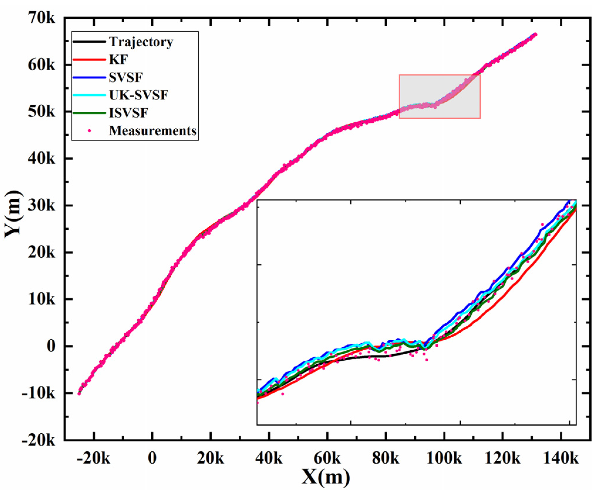
where “w.p.” is short for “with probability”, the Kalman filter is the optimal filter when the system and measurement noise are white, and the initial state conditions have known means and variances [45]. However, for agile targets, the process noise is difficult to model in advance, which means that the random acceleration of the target is unknown. The simulation of the random acceleration follows a Gaussian distribution with 10   m / s 2 standard deviation. The real trajectory is shown in Figure 5. Additionally, in the simulation, all filters use the uniform motion model, and the parameter L of Q is set to 1 in the ISVSF, UK-SVSF and KF. The smooth boundary layer widths of the SVSF, UK-SVSF and ISVSF are set to ψ = [ 2 000 , 2000 ]   m . The κ of the UK-SVSF is set to κ = 3 n x , and ψ f i x e d = 3200   m . Under the same measurement noise distributions, 400 Monte Carlo runs are performed.
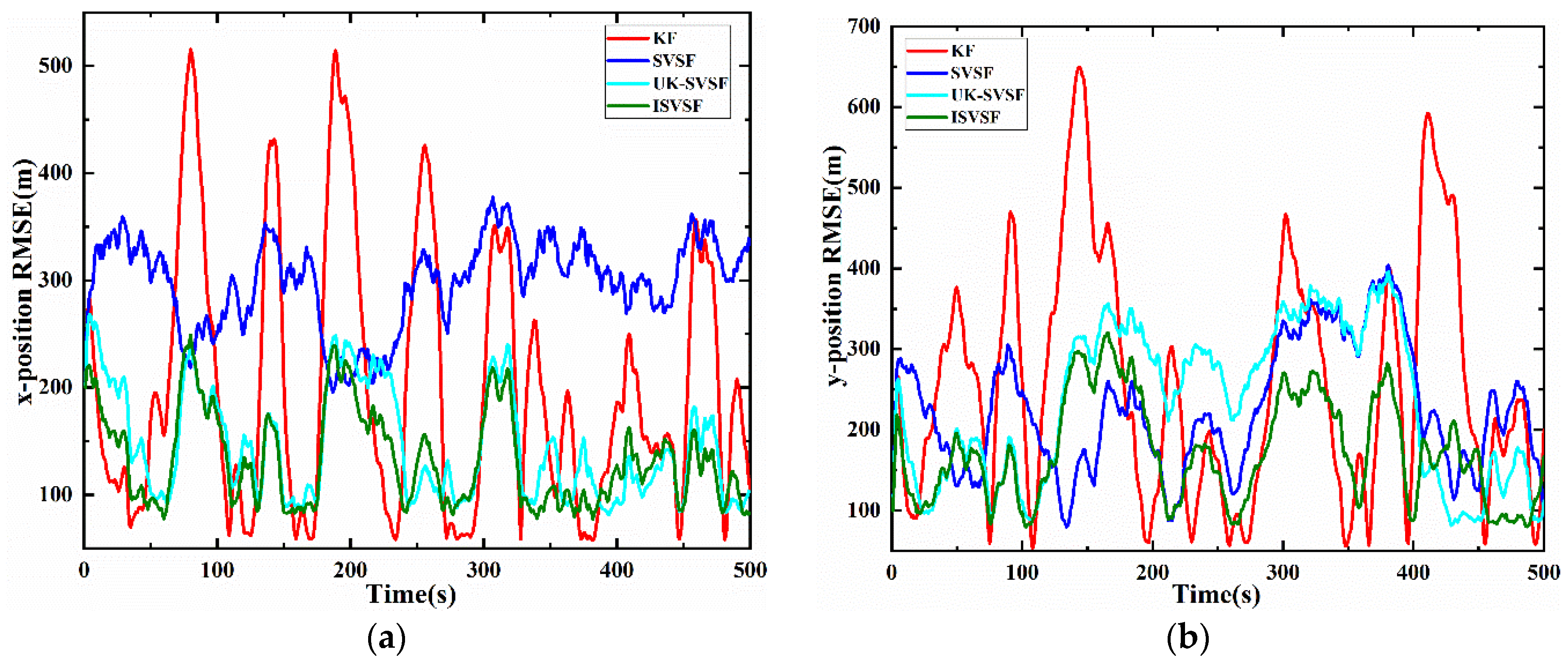
Figure 5 shows the trajectory of one simulation result, including the real trajectory, the points of measurement and the trajectory processed by the filters. Additionally, the small diagram contained in Figure 5 is a partially enlarged one. It can be seen from Figure 5 that the trajectory obtained by the ISVSF is more approximate to the real trajectory. From Figure 6 and Table 2, the ARMSE of the ISVSF is the least compared with the KF, SVSF and UK-SVSF. For use of the KF, knowledge of an accurate mathematical model and the statistical characteristics of system noise and measurement noise is required to obtain the desired filtering effect. Compared with the SVSF, UK-SVSF and ISVSF, the performance of the KF is more unstable when the acceleration noise disturbance is underestimated and the measurement noise is unknown. The SVSF has a stable filtering effect, but its ability to eliminate noise should be improved. The ISVSF has a better filtering effect than the SVSF, as shown in Table 2, and the position ARMSE of the ISVSF is reduced by above 60% compared with the SVSF. The ISVSF not only has higher tracking accuracy compared with the SVSF but also has higher robustness than the KF under unknown noises. Although the UK-SVSF improves the robustness and accuracy under unknown noises, the velocity estimation is affected due to competition between the UKF and SVSF. Compared with the SVSF, the accuracy of the ISVSF is improved because of its highly accurate velocity estimation.

4.1.2. Results under the Condition of Different Smooth Boundary Layer Widths

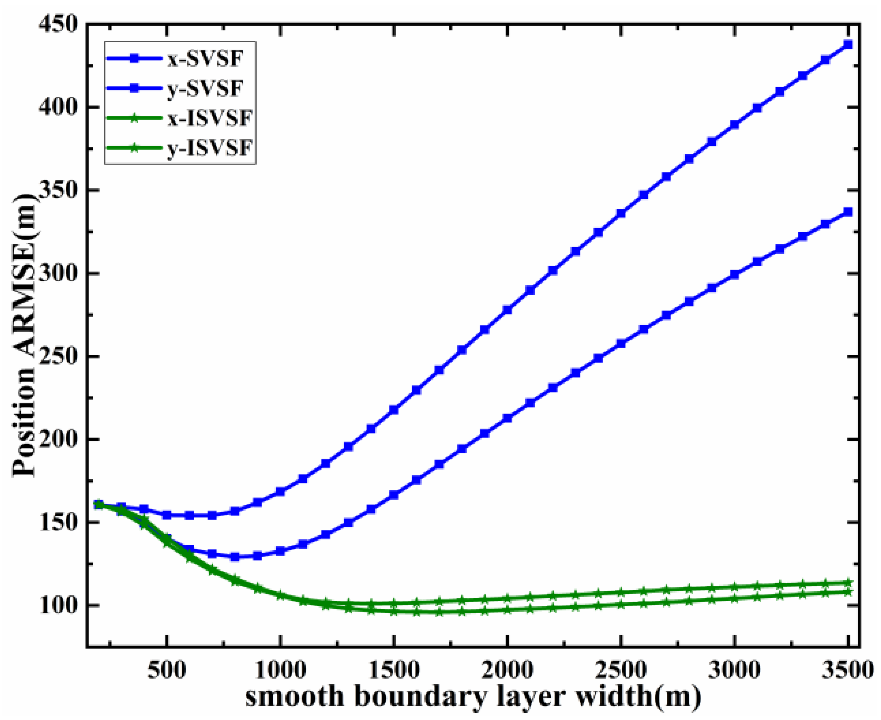
Smooth boundary layer width is an important parameter in systems based on the SVSF, and its value setting will affect the stability and accuracy of the system. To verify this influence, the range of smooth boundary layer width is set from 200   m to 3500   m at intervals of 100   m . From Figure 7, the results show that when the smooth boundary layer width is less than the existence subspace layer, the precision of the ISVSF and SVSF will be affected because of the existing chattering. With the smooth boundary layer width increasing, SVSF ARMSE decreases slightly first, and then increases sharply as shown in Figure 7. The reason is that the SVSF lacks estimation of the velocity dimension of the state, which causes the SVSF to commit a large error in model extrapolation. The fact that the accuracy of ISVSF is less susceptible to the smooth boundary layer width than SVSF can be attributed to the Bayesian filtering estimation, which can estimate velocity so that the predicted trajectory of ISVSF is closer to the real trajectory than that of SVSF on the prediction stage, which decrease prediction errors, ensuring the accuracy and thus maintaining the stability. How to effectively use the ISVSF to modify the velocity information will be described in the following passage. The combination with the Bayesian filtering process can eliminate the impact of the smooth boundary layer width and deliver more stable filtering results.

4.2. Simulation Results in Modeling Error

Given the high accuracy requirements of most filters for mathematical models, a system divergence will occur once the modeling of the filter is wrong. When tracking the maneuvering target, the system model is uncertain and often inconsistent with the actual model. F is state space model of the system matrix and F c is the changing model; they are defined as follows:
F = [ 1 T 0 0 0 1 0 0 0 0 1 T 0 0 0 1 ] F c = [ 1 sin ( wT ) / w 0 ( cos ( wT ) 1 ) / w 0 cos ( wT ) 0 sin ( wT ) 0 ( 1 cos ( wT ) ) / w 1 sin ( wT ) / w 0 sin ( wT ) 0 cos ( wT ) ]
In the target tracking, F represents uniform motion and F c represents a uniform turning motion with an angular velocity of w . The initial position of the target is [ 25,000   m ,   10,000   m ] , and the target moves in a straight line at a uniform velocity of [ 320   m / s , 20   m / s ] for 100   s . Then, the maneuvering target turns at a rate of 3 ° / s for 60   s . Next, the target moves in a straight line at a uniform velocity for 90   s , and maneuvers at a rate of 2 ° / s for 90   s . Finally the target flies straight for 160 s until the end. No matter whether they are on the x-axis and y-axis, noises of measurements obey a Gaussian distribution with standard deviation of 200 m. In order to assess its performance, a total of 300 Monte Carlo runs are carried out. The simulation is conducted to test the robustness of three strategies in modeling errors.
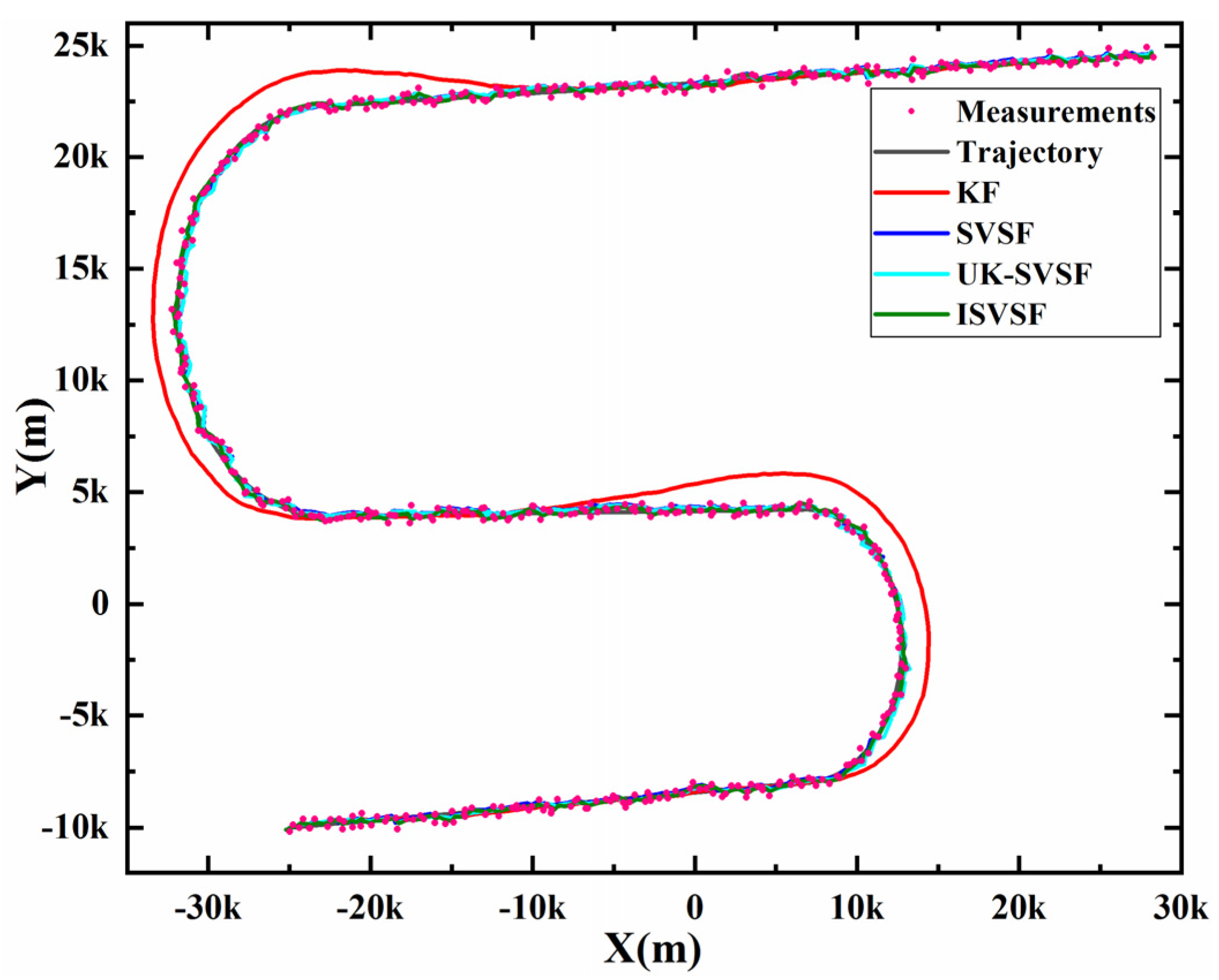
In the simulation, the smooth boundary layer widths of the ISVSF, UK-SVSF and SVSF are set to ψ = [ 1200   m , 1200   m ] , the L of the KF and UK-SVSF are set to 1, the κ of UK-SVSF is set to κ = 3 n x , ψ f i x e d is set to ψ f i x e d = 3200 and x 0 = [ 25,000   m , 220   m / s , 10,000   m , 60   m / s ] , the L of the ISVSF is set to 1000, and other parameters are similar to the above simulation. The simulation results are as follows: Figure 8 shows the trajectory of one simulation result, including the real trajectory, and the points of measurement and the trajectory are processed by three filters. Figure 8 and Figure 9a,b show that, when the model is unchanged, the KF would achieve the best performance in velocity and position estimation; when the modeling of the filter is different from the motion model of the target, the position RMSE of the ISVSF, UK-SVSF and SVSF would increase slightly, while the position RMSE of the KF would increase greatly. As shown in Figure 9b, the original SVSF does not estimate the velocity, and the velocity error of SVSF is induced by the difference between the initial velocity of the SVSF and the actual velocity of the target, but the KF and ISVSF can eliminate this error through iterative calculation. Compared with the SVSF, the ISVSF adds the Bayesian solution process and can thereby estimate velocity more accurately. It can be seen from the Table 3 that the velocity ARMSE of the ISVSF is 3.6 times less than that of the SVSF. The result also shows that the UK-SVSF has improved estimation accuracy and stability. When the modeling has an error under the maneuvering condition, the UK-SVSF method mainly uses the SVSF to estimate state, and the error in estimated velocity is large because the SVSF is deficient in estimating velocity, and a certain competition and interference also exist between the UKF and SVSF. Compared with the ISVSF, the UK-SVSF performs better under normal conditions, while the ISVSF is better if modeling uncertainty exists. To sum up, the ISVSF, UK-SVSF and SVSF all have good robustness. However, compared with the UK-SVSF and SVSF, the ISVSF has better filtering performance.

4.3. A Comprehensive Simulation

Some uncertain factors could influence systems and change system parameters or states. For example, if the target is impacted by external factors such as strong external impact, disturbance or occlusions, its state will change greatly when it is detected again. In the fault diagnosis system, the parameters and state of the characterization system will change dramatically once a fault occurs [8]. That is, in some particular case, one may expect a substantial deviation of the assumed system description from the true one [7]. An application example is shown in Appendix A. The comprehensive simulation is presented as follows. It contains different kinds of maneuvering and sudden changes caused by interference. The purpose is to test the robustness and accuracy of the proposed ISVSF. Additionally, a comparison has been made between the ISVSF and other methods to estimate states without measurement in the case where the measurement vector is less than the state vector.
In the simulation, the actual measurement noise is expressed as follows:
v k = { N ( 0 , 200 2 )     w . p .   0.90 N ( 0 , 9 × 200 2 )     w . p .   0.10
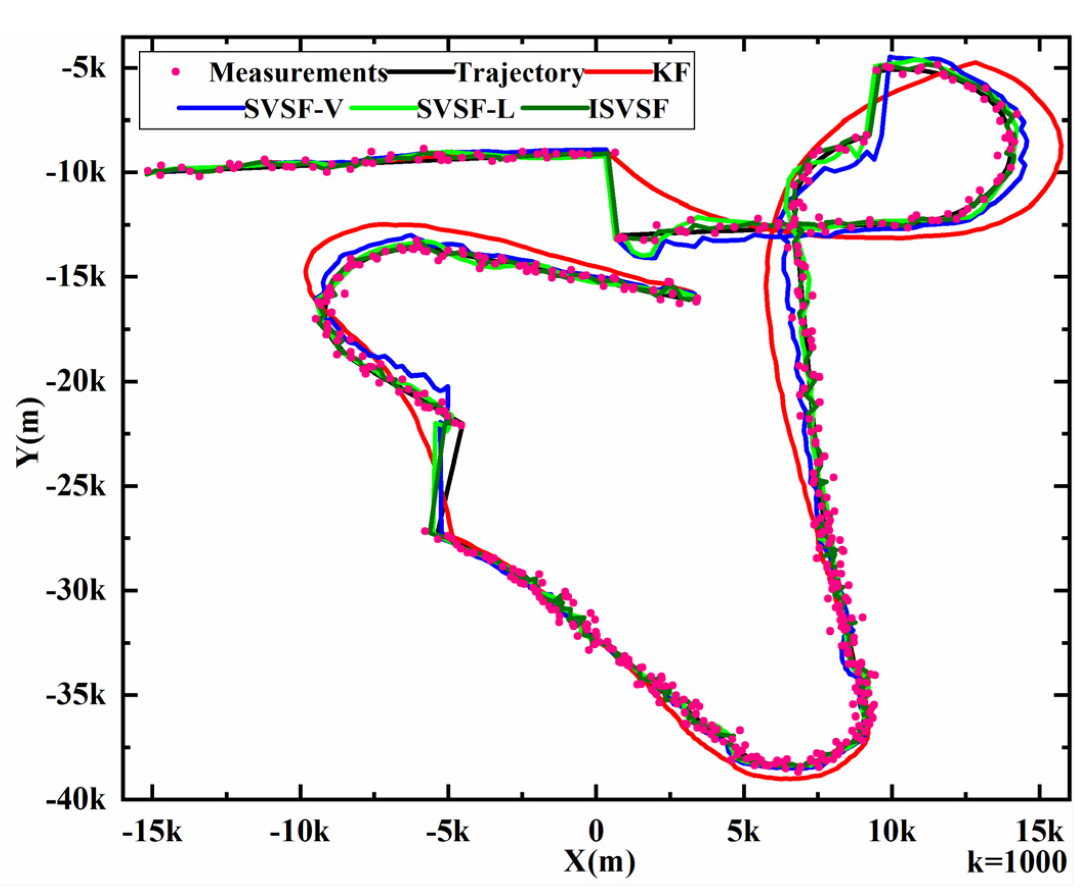
The movement parameters for a maneuvering target in this simulation are listed in Table 4, and the real trajectory is shown in Figure 10.
In the simulation, the SVSF with Luenberger’s strategy (SVSF-L) [24,26] and the SVSF with “artificial” velocity measurements (SVSF-V) [17,21] are applied to estimate velocity. The SVSF and UK-SVSF have large estimation errors when the target maneuvers, so they are not shown in the simulations. The position smooth boundary layer width of the ISVSF, SVSF-L and SVSF-V are set to [ 3000 , 3000 ] , the velocity smooth boundary layer width of SVSF-L and SVSF-V are set to [ 5400 , 5400 ] , and other parameters are similar to those in above simulation 4.2. In order to assess its performance, 1000 Monte Carlo simulations were carried out.
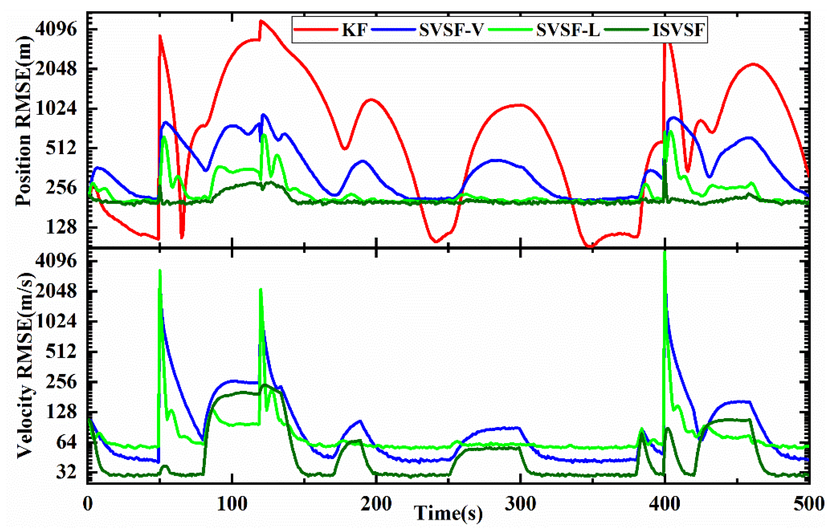
Figure 10 shows the trajectories of one simulation, including the real trajectory, measurements and the trajectories obtained by different methods. All filters use the uniform motion model. It can be seen from Figure 10 and Figure 11 that those methods based on the SVSF have good robustness in systems with modeling errors. Compared with the ISVSF and SVSF-L, the SVSF-V is more vulnerable to noise and maneuvering because its “artificial” velocity measurement is obtained by dividing the position differences in one cycle by the sampling time, so that the “artificial” velocity is easily affected by noise and thus produce a larger errors. From Figure 11, when sudden position changes occur at 50 s, 120 s and 400 s, both the SVSF-L and SVSF-V have large velocity estimation errors, especially the SVSF-L. All of the position estimation errors of the SVSF-L, SVSF-V and ISVSF are smaller than the change in position values. However, the proposed ISVSF is more stable and can quickly converge to a steady state. That can be attributed to the fact that in the first step, the ISVSF can adapt to a sudden change in position state without affecting the covariance of the velocity dimension, which ensures that in the second step, the estimation performance of the ISVSF obtains a more accurate velocity. In the case of weak maneuvering, the ISVSF and SVSF-L have minor estimation errors compared with the SVSF-V. The three methods based on the SVSF all have their own advantages when estimating states without measurement in the case where the measurement vector is less than the state vector, and the three methods can be chosen according to different requirements, Besides that, the ISVSF has another advantage in that there is no need to set smoothing layer width for unmeasured states. It can be concluded from Table 5 that the ISVSF has a smaller ARMSE than the other methods under 1000 simulations. To sum up, the ISVSF has good robustness and accuracy.

5. Conclusions

This paper proposes an improved SVSF (ISVSF) that combines Bayesian theory and the SVSF. The ISVSF uses the SVSF theory to make preliminary estimations, then, using the derived covariance and Bayesian theory, makes further estimations. It is capable not only of maintaining the robustness of the SVSF but also of retaining the advantages of the Bayesian filtering system. Moreover, it can estimate the lower dimension states that have no corresponding measurement value. A performance comparison of the ISVSF, UK-SVSF, KF and SVSF indicates that the ISVSF achieves improved performance under the conditions of modeling error and unknown noise. Even if state undergoes a sudden change in the presence of external factors, the ISVSF still shows satisfactory performance. We hope that further research can be conducted to unleash the great potential of the ISVSF and SVSF in applications involving more complex and changeable systems.

Author Contributions

Data curation, Y.C.; Formal analysis, Y.C., G.W. and B.Y.; Funding acquisition, L.X., G.W. and J.S.; Project administration, L.X.; Resources, J.S.; Software, B.Y.; Supervision, L.X.; Writing—original draft, Y.C. All authors have read and agreed to the published version of the manuscript.

Funding

This work was supported by National Natural Science Foundation of China (No. 62071363, 61701383), China Postdoctoral Science Foundation (No. 2019M663633), Natural Science Basic Research Plan in Shaanxi Province of China (No. 2018JQ6100), Fundamental Research Funds for the Central Universities (No. JB211310), Key Laboratory of Cognitive Radio and Information Processing Ministry of Education 2019 open fund project (No. CRKL190203, Guilin University of Electronic Technology).

Acknowledgments

The author is grateful to Yeting Shi for revising English.

Conflicts of Interest

The authors declare no conflict of interest.

Appendix A. The Application of ISVSF in a System with State Undergoing a Sudden Change
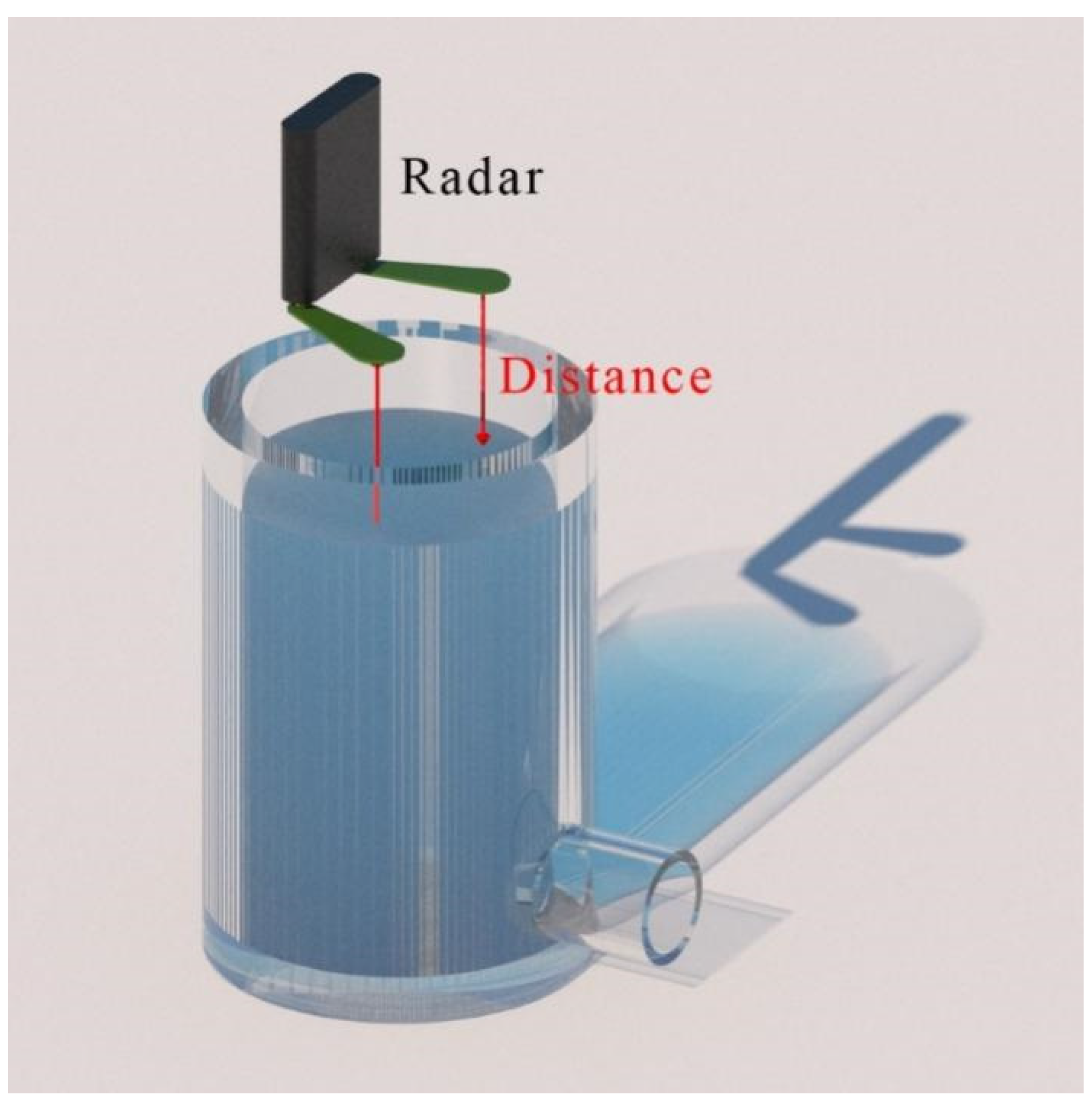
A real-time monitoring system of liquid level uses a frequency modulated continuous wave radar to obtain the liquid height and filling velocity, such as shown in Figure A1 and A2. The tank is filled by the top pump with the reaction solution at an unknown velocity. The reaction liquid is discharged through the bottom valve, so that the liquid level drops rapidly. The radar system can only detect the height measurement of the liquid, but in most circumstances, the real-time liquid filling velocity is also required. The initial distance between the radar and the liquid level is 500   cm at t = 0   min . As the reaction solution fills the tank, the liquid level rise at the velocity of 20   cm / min . At t = 19   min and t = 39   min , the valve opens and the liquid level drops rapidly at 400   cm . The radar sampling period is T = 1   min , and the measurement error obeys the Gauss distribution with the standard deviation of 10 cm.
Figure A1. Radar liquid level monitoring system.
Remotesensing 13 04612 g0a1
The behavior of a monitoring system can be modeled as follows:
x k + 1 = [ 1 T 0 1 ] x k + [ 1 2 T 2 T ] w k + g k
The state vector may be defined as follows:
x k = [ η k , η ˙ k ] T , w k = [ η ¨ k ]
where η k is the distance between liquid level and radar, and η ˙ k is the rising velocity of the liquid level.
g k = { [ 400 , 0 ] T   k = 19 , 39 [ 0 , 0 ] T   k = else
Because the radar only provides height measurements, the measurement equation can be defined as follows:
z k = [ 1   0 ] x k + v k
The process and measurement noise ( w k , v k ) are considered as Gaussian with zero mean and variances, which can be represented by Q and R . The system initial x 0 , P 0 , R and Q are defined as follows:
X 0 = [ 520 , 0 ] T , P 0 = diag ( [ 100 , 400 ] ) , R = 10 2
Q = 1 [ T 3 3 T 2 2 T 2 2 T ]
The original SVSF cannot estimate velocity directly, and the inflow velocity of the reaction liquid is required in real cases. To tackle this issue, one approach is to add an ‘artificial’ velocity measurement in the SVSF. The ‘artificial’ velocity measurement can be calculated through height measurements. For example, where y k represents the height measurement, artificial velocity measurements can be expressed as follows [17]:
y k = [ z k , ( z k z k 1 ) / T ] T
It is also necessary to transform the measurement matrix of (A4) into a square matrix (i.e., identity). In this paper, artificial velocity measurements are added to the SVSF, and the method is labelled as SVSF-V.
The smooth boundary layer widths of SVSF, UK-SVSF and ISVSF are set to ψ = [ 50 ] , and of SVSF-V to ψ = [ 50 , 250 ] , and the SVSF, SVSF-V, UK-SVSF and ISVSF convergence rates are set to γ = 0.1 . The κ of the ISVSF is set to κ = 3 n x and the ψ f i x e d is set to ψ f i x e d = 50 . The estimations of the KF, SVSF, SVSF-V and ISVSF were conducted by using the UM model in a total of 200 runs.
Figure A2. Height trajectory of one experiment.
Remotesensing 13 04612 g0a2
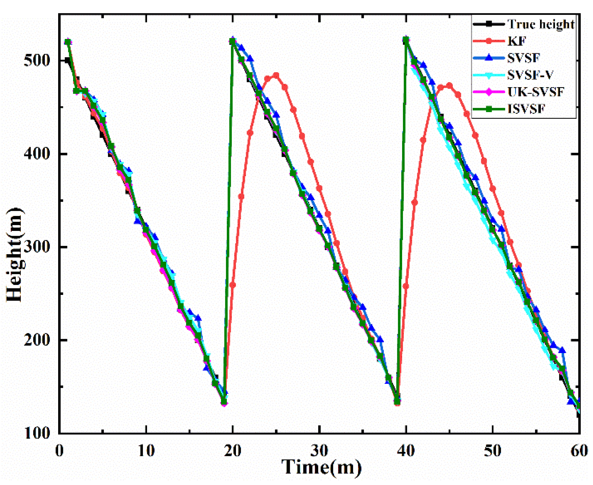
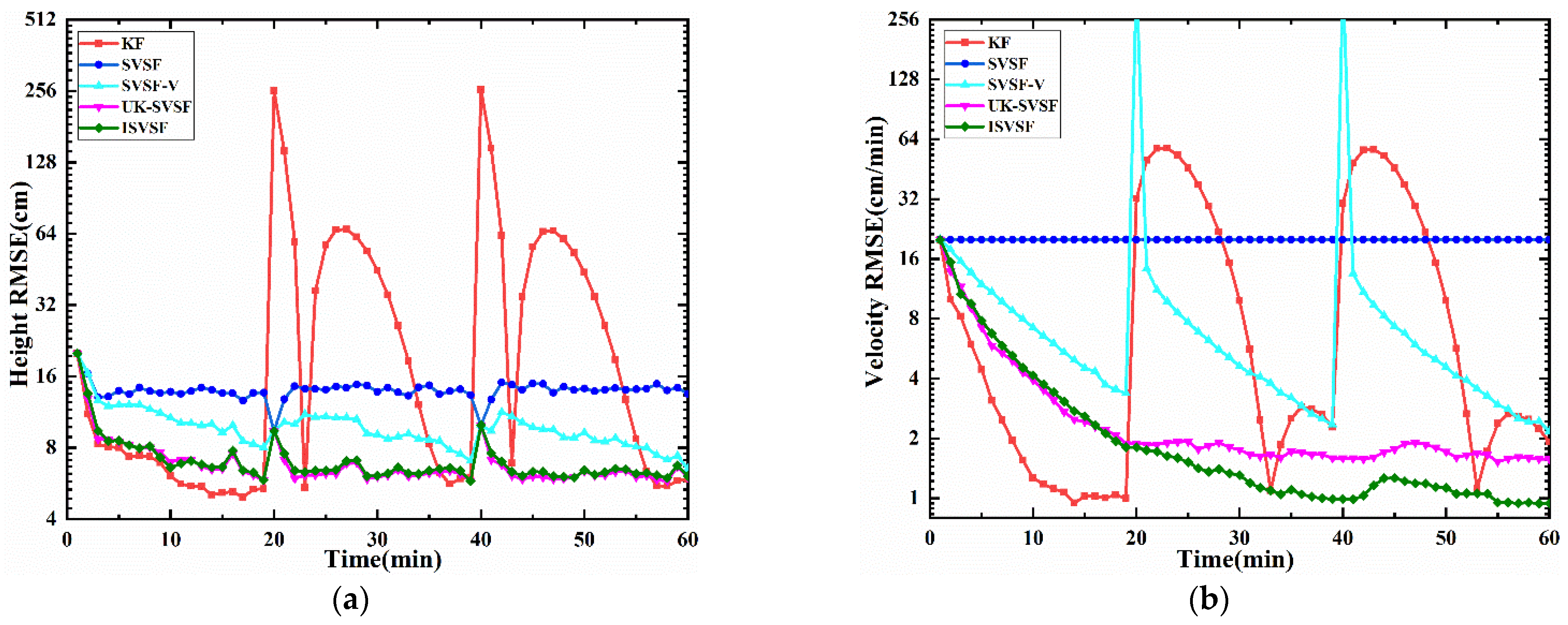
The results of different estimation methods are shown in Figure A2 and Figure A3 and Table A1. From Figure A2, it can be seen that the height trajectory estimated by the UK-SVSF and ISVSF are closer to the real value than other methods. From Figure A3a,b, it can be seen that the KF has the best performance when the parameter matches the system ( 0 19   min ), but when the value of the height state in the system changes suddenly at 20 min, the performance of the KF estimation decreases significantly. The original SVSF has a stable estimation of height, but the estimation is inaccurate because it cannot estimate the velocity, which can be reflected by the fixed velocity error shown in Figure A3b. After the SVSF adds artificial velocity measurements (SVSF-V), the performance of the SVSF-V is improved compared with that of the SVSF. However, when the value of the height state suddenly increases by 400   cm , a more serious velocity error will occur, and the estimation results will be affected. Compared with other methods, the ISVSF and UK-SVSF have better estimation results. For the ISVSF, the reason can be attributed to the fact that in the first step, the ISVSF can adapt to a sudden change in height state without affecting the covariance of the velocity dimension, which ensures that in the second step, the estimation performance of the ISVSF can obtain a more accurate liquid filling velocity. From Table 4, compared with the SVSF and SVSF-V, the velocity of ISVSF ARMSE is reduced by more than 8 times. The UK-SVSF and ISVSF excel because they can handle unknown state value changes and show fair robustness as well as accuracy, but the ISVSF yields more accurate velocity estimations than does the UK-SVSF.
Table A1. The ARMSE of estimation states.
Different MethodsKFSVSFSVSF-VUK-SVSFISVSF
Height ARMSE (cm)35.014.09.86.97.1
Velocity ARMSE (cm/min)15.52019.72.52.2
Figure A3. Position RMSE and velocity RMSE of estimation result. (a) Position RMSE; (b) velocity RMSE.
Remotesensing 13 04612 g0a3

References

  1. Li, X.R.; Jilkov, V.P. Survey of maneuvering target tracking. Part V. Multiple-model methods. IEEE Trans. Aerosp. Electron. Syst. 2005, 41, 1255–1321. [Google Scholar]
  2. Patwardhan, S.C.; Narasimhan, S.; Jagadeesan, P.; Gopaluni, B.; Shah, S.L. Nonlinear Bayesian state estimation: A review of recent developments. Control. Eng. Pr. 2012, 20, 933–953. [Google Scholar] [CrossRef]
  3. Kalman, R.E. A New Approach to Linear Filtering and Prediction Problems. J. Basic Eng. 1960, 82, 35–45. [Google Scholar] [CrossRef] [Green Version]
  4. Gao, R.; Tronarp, F.; Sarkka, S. Iterated Extended Kalman Smoother-Based Variable Splitting for L1-Regularized State Estimation. IEEE Trans. Signal Process. 2019, 67, 5078–5092. [Google Scholar] [CrossRef] [Green Version]
  5. Asgari, M.; Khaloozadeh, H. Robust extended Kalman filtering for non-linear systems with unknown input: A UBB model approach. IET Radar Sonar Navig. 2020, 14, 1837–1844. [Google Scholar] [CrossRef]
  6. Chang, L.; Hu, B.; Li, A.; Qin, F. Transformed Unscented Kalman Filter. IEEE Trans. Autom. Control. 2013, 58, 252–257. [Google Scholar] [CrossRef]
  7. Gadsden, S.; AlShabi, M.; Arasaratnam, I.; Habibi, S. Combined cubature Kalman and smooth variable structure filtering: A robust nonlinear estimation strategy. Signal Process. 2014, 96, 290–299. [Google Scholar] [CrossRef]
  8. Zhang, Z.; Chen, J. Fault detection and diagnosis based on particle filters combined with interactive multiple-model estimation in dynamic process systems. ISA Trans. 2019, 85, 247–261. [Google Scholar] [CrossRef] [PubMed]
  9. Qin, H.; Xue, X.; Yang, Q. GNSS multipath estimation and mitigation based on particle filter. IET Radar Sonar Navig. 2019, 13, 1588–1596. [Google Scholar] [CrossRef]
  10. Jondhale, S.R.; Deshpande, R.S. GRNN and KF framework based real time target tracking using PSOC BLE and smartphone. Ad Hoc Netw. 2019, 84, 19–28. [Google Scholar] [CrossRef]
  11. Jondhale, S.R.; Deshpande, R.S. Kalman Filtering Framework-Based Real Time Target Tracking in Wireless Sensor Networks Using Generalized Regression Neural Networks. IEEE Sens. J. 2019, 19, 224–233. [Google Scholar] [CrossRef]
  12. Li, X.-R.; Bar-Shalom, Y. Multiple-model estimation with variable structure. IEEE Trans. Autom. Control. 1996, 41, 478–493. [Google Scholar] [CrossRef]
  13. Huang, H.; Tang, J.; Zhang, B.; Chen, J.; Zhang, J.; Song, X. A Novel Nonlinear Algorithm for Non-Gaussian Noises and Measurement Information Loss in Underwater Navigation. IEEE Access 2020, 8, 118472–118484. [Google Scholar] [CrossRef]
  14. He, J.; Sun, C.; Zhang, B.; Wang, P. Maximum Correntropy Square-Root Cubature Kalman Filter for Non-Gaussian Measurement Noise. IEEE Access 2020, 8, 70162–70170. [Google Scholar] [CrossRef]
  15. Huang, Y.; Zhang, Y.; Zhao, Y.; Chambers, J.A. A Novel Robust Gaussian–Student’s t Mixture Distribution Based Kalman Filter. IEEE Trans. Signal Process. 2019, 67, 3606–3620. [Google Scholar] [CrossRef]
  16. Habibi, S. The Smooth Variable Structure Filter. Proc. IEEE 2007, 95, 1026–1059. [Google Scholar] [CrossRef]
  17. Gadsden, S.A.; Habibi, S.; Kirubarajan, T. Kalman and smooth variable structure filters for robust estimation. IEEE Trans. Aerosp. Electron. Syst. 2014, 50, 1038–1050. [Google Scholar] [CrossRef]
  18. Gadsden, S.A.; Habibi, S.R. A new form of the smooth variable structure filter with a covariance derivation. In Proceedings of the 49th IEEE Conference on Decision and Control (CDC), Atlanta, GA, USA, 15–17 December 2010; pp. 7389–7394. [Google Scholar]
  19. Gadsden, S.A.; Habibi, S.R. A New Robust Filtering Strategy for Linear Systems. J. Dyn. Syst. Meas. Control. 2013, 135, 014503. [Google Scholar] [CrossRef]
  20. Ma, A.; Ah, A.; Asb, C.; Sag, C. The smooth variable structure filter: A comprehensive review. Digit. Signal Process. 2020, 110, 102912. [Google Scholar]
  21. AlShabi, M.; Gadsden, S.; Habibi, S. Kalman filtering strategies utilizing the chattering effects of the smooth variable structure filter. Signal Process. 2013, 93, 420–431. [Google Scholar] [CrossRef]
  22. Spiller, M.; Bakhshande, F.; Soeffker, D. The uncertainty learning filter: A revised smooth variable structure filter. Signal Process. 2018, 152, 217–226. [Google Scholar] [CrossRef]
  23. Afshari, H.H.; Gadsden, S.A.; Habibi, S. A nonlinear second-order filtering strategy for state estimation of uncertain systems. Signal Process. 2019, 155, 182–192. [Google Scholar] [CrossRef]
  24. Luo, Z.; Attari, M.; Habibi, S.; Von Mohrenschildt, M. Online Multiple Maneuvering Vehicle Tracking System Based on Multi-Model Smooth Variable Structure Filter. IEEE Trans. Intell. Transp. Syst. 2020, 21, 603–616. [Google Scholar] [CrossRef]
  25. Youn, W.; Gadsden, S.A. Combined Quaternion-Based Error State Kalman Filtering and Smooth Variable Structure Filtering for Robust Attitude Estimation. IEEE Access 2019, 7, 148989–149004. [Google Scholar] [CrossRef]
  26. Attari, M.; Habibi, S.; Gadsden, S.A. Target Tracking Formulation of the SVSF With Data Association Techniques. IEEE Trans. Aerosp. Electron. Syst. 2017, 53, 12–25. [Google Scholar] [CrossRef]
  27. Attari, M.; Luo, Z.; Habibi, S. An SVSF-Based Generalized Robust Strategy for Target Tracking in Clutter. IEEE Trans. Intell. Transp. Syst. 2016, 17, 1381–1392. [Google Scholar] [CrossRef]
  28. Demim, F.; Nemra, A.; Boucheloukh, A.; Kobzili, E.; Hamerlain, M.; Bazoula, A. SLAM based on Adaptive SVSF for Cooperative Unmanned Vehicles in Dynamic environment. IFAC PapersOnLine 2019, 52, 73–80. [Google Scholar] [CrossRef]
  29. Patra, N.; Sadhu, S.; Ghoshal, T.K. Adaptive state estimation for tracking of civilian aircraft. IET Sci. Meas. Technol. 2018, 12, 777–784. [Google Scholar] [CrossRef]
  30. Demim, F.; Nemra, A.; Louadj, K.; Hamerlain, M.; Bazoula, A. Cooperative SLAM for multiple UGVs navigation using SVSF filter. Automatika 2017, 58, 119–129. [Google Scholar] [CrossRef] [Green Version]
  31. Cao, L.; Chen, Y.; Zhang, Z.; Li, H.-N.; Misra, A.K. Predictive Smooth Variable Structure Filter for Attitude Synchronization Estimation During Satellite Formation Flying. IEEE Trans. Aerosp. Electron. Syst. 2017, 53, 1375–1383. [Google Scholar] [CrossRef]
  32. Gadsden, S.A.; Song, Y.; Habibi, S.R. Novel Model-Based Estimators for the Purposes of Fault Detection and Diagnosis. IEEE/ASME Trans. Mechatron. 2013, 18, 1237–1249. [Google Scholar] [CrossRef]
  33. Ahmed, R.; El Sayed, M.; Gadsden, S.A.; Tjong, J.; Habibi, S. Automotive Internal-Combustion-Engine Fault Detection and Classification Using Artificial Neural Network Techniques. IEEE Trans. Veh. Technol. 2015, 64, 21–33. [Google Scholar] [CrossRef]
  34. Ahmed, R.; El Sayed, M.; Arasaratnam, I.; Tjong, J.; Habibi, S. Reduced-Order Electrochemical Model Parameters Identification and State of Charge Estimation for Healthy and Aged Li-Ion Batteries—Part II: Aged Battery Model and State of Charge Estimation. IEEE J. Emerg. Sel. Top. Power Electron. 2014, 2, 678–690. [Google Scholar] [CrossRef]
  35. Alshabi, M.; Elnady, A. Recursive Smooth Variable Structure Filter for Estimation Processes in Direct Power Control Scheme Under Balanced and Unbalanced Power Grid. IEEE Syst. J. 2020, 14, 971–982. [Google Scholar] [CrossRef]
  36. Xu, X.; Lin, Y.; Wang, F.; Yang, S.; Zhou, Z. A hybrid observer for SOC estimation of lithium-ion battery based on a coupled electrochemical-thermal model. Int. J. Green Energy 2019, 16, 1527–1538. [Google Scholar] [CrossRef]
  37. Afshari, H.H.; Attari, M.; Ahmed, R.; Delbari, A.; Habibi, S.; Shoa, T. Reliable state of charge and state of health estimation using the smooth variable structure filter. Control. Eng. Pr. 2018, 77, 1–14. [Google Scholar] [CrossRef]
  38. Ismail, M.; Attari, M.; Habibi, S.; Ziada, S. Estimation theory and Neural Networks revisited: REKF and RSVSF as optimization techniques for Deep-Learning. Neural Netw. 2018, 108, 509–526. [Google Scholar] [CrossRef]
  39. Ahmed, R.; El Sayed, M.; Gadsden, S.A.; Tjong, J.; Habibi, S. Artificial neural network training utilizing the smooth variable structure filter estimation strategy. Neural Comput. Appl. 2016, 27, 537–548. [Google Scholar] [CrossRef]
  40. Arasaratnam, I.; Haykin, S. Cubature kalman filters. IEEE Trans. Autom. Control 2009, 54, 1254–1269. [Google Scholar] [CrossRef] [Green Version]
  41. Chen, Y.; Xu, L.; Yan, B.; Li, C. A Novel Smooth Variable Structure Smoother for Robust Estimation. Sensors 2020, 20, 1781. [Google Scholar] [CrossRef] [PubMed] [Green Version]
  42. Habibi, S.R.; Burton, R.M. The Variable Structure Filter. J. Dyn. Syst. Meas. Control. 2003, 125, 287–293. [Google Scholar] [CrossRef]
  43. Al-Shabi, M.; Hatamleh, K.S.; Gadsden, S.A.; Soudan, B.; El-Nady, A. Robust nonlinear control and estimation of a prrr robot system. Int. J. Robot. Autom. 2019, 34, 632–644. [Google Scholar] [CrossRef]
  44. Avzayesh, M.; Abdel-Hafez, M.F.; Al-Masri, W.M.F.; Alshabi, M.; El-Hag, A.H. A Hybrid Estimation-Based Technique for Partial Discharge Localization. IEEE Trans. Instrum. Meas. 2020, 69, 8744–8753. [Google Scholar] [CrossRef]
  45. Grewal, M.; Andrews, A. Kalman Filtering: Theory and Practice with MATLAB, 4th ed.; John Wiley & Sons: Hoboken, NJ, USA, 2015. [Google Scholar]
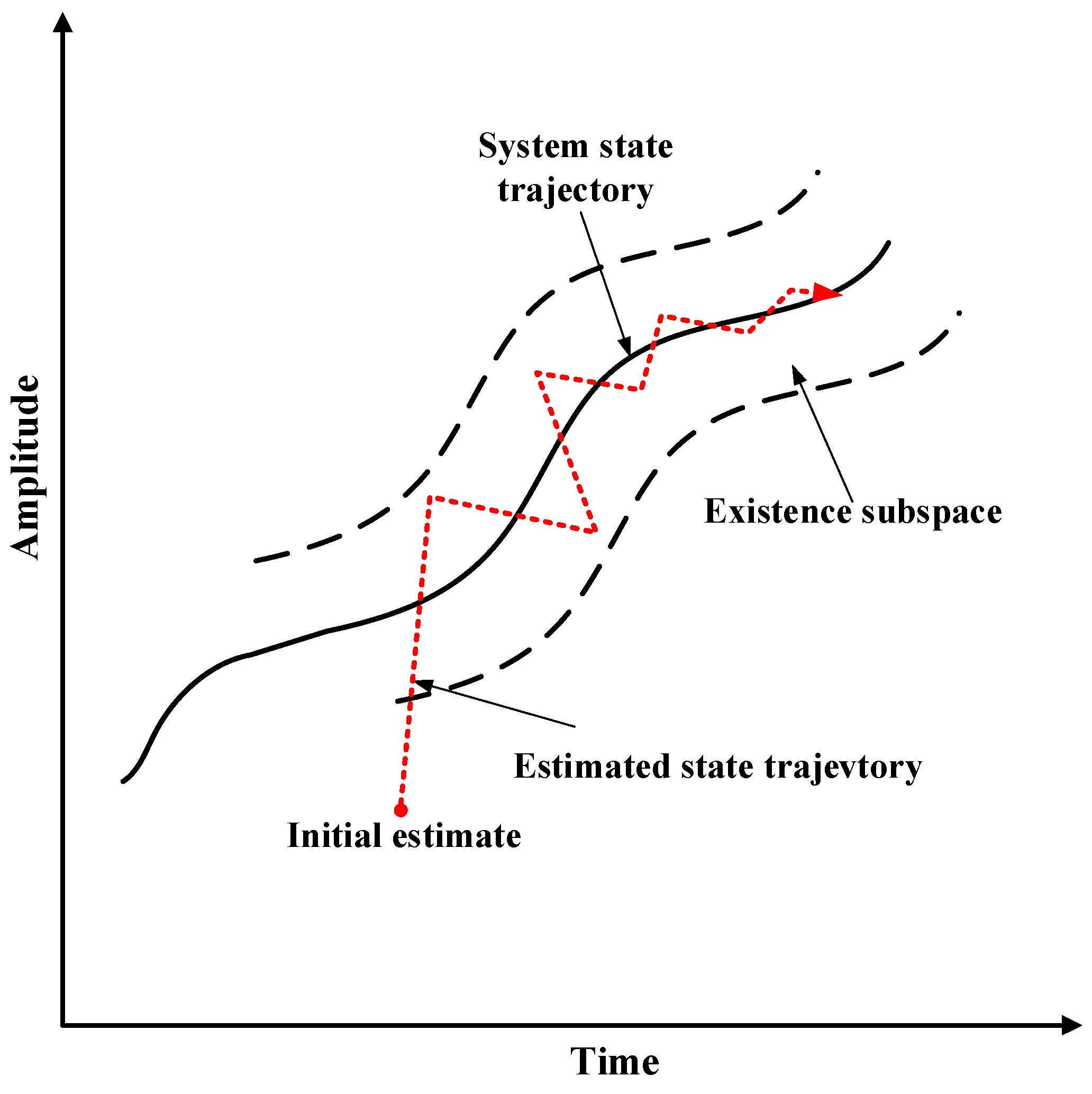
Figure 1. SVSF estimation concept [16].
Remotesensing 13 04612 g001
Figure 2. Smoothing boundary layer concept, adapted from [16]: (a) chattering effect ( ψ β ); (b) Smoothed estimated trajectory ( ψ > β ).
Remotesensing 13 04612 g002
Figure 3. (a) Methodology for combining the SVSF with other estimation strategies, adapted from [20]; (b) flowchart of the proposed ISVSF.
Remotesensing 13 04612 g003
Figure 4. ISVSF algorithm block diagram.
Remotesensing 13 04612 g004
Figure 5. Position trajectory of one experiment.
Remotesensing 13 04612 g005
Figure 6. RMSE of position on x-axis and y-axis (m). (a) RMSE of position on x-axis; (b) RMSE of position on y-axis.
Remotesensing 13 04612 g006
Figure 7. The position ARMSE of different ψ on the x-axis and y-axis (m).
Remotesensing 13 04612 g007
Figure 8. Position trajectory of one experiment.
Remotesensing 13 04612 g008
Figure 9. Position RMSE and velocity RMSE of estimation result. (a) Position RMSE; (b) velocity RMSE.
Remotesensing 13 04612 g009
Figure 10. Position trajectories of one simulation.
Remotesensing 13 04612 g010
Figure 11. Position RMSE and velocity RMSE of estimation result.
Remotesensing 13 04612 g011
Table 1. The SVSF Strategies.
SymbolDefinition
^Notation denoting an estimated variable, function, or model parameter
~Notation denoting the error in an estimated variable, function, or model parameter
F , F ^ , F ˜ System model, mathematical modeling, and modeling error
H measurement (out) matrix
x k , x ^ k , x ˜ k System state, prior estimate state, state error
e k + 1 | k svsf , e k + 1 | k + 1 svsf The priori and posterior measurement innovation of SVSF
e k + 1 | k + 1 A posterior error
diag Diagonal of vector or matrix
sat Saturation function
Q , R System and measurement covariance matrix
| e | Absolute value of e
+Pseudoinverse of some non-square matrix
Indication or Hadamard product
T Transpose of a vector or sample rate
ψ SVSF smoothing boundary layer
n Matrix dimension
K k + 1 svsf SVSF gain matrix
K k + 1 Bayes’ rule gain
E Expectation
f , h Nonlinear function
γ SVSF “memory” or convergence
p Probability density function
β Existence subspace layer
P State error covariance matrix
z k Measurement (system output) matrix
w , v System noise and measurement noise vector
Table 2. The position ARMSE on the x-axis and y-axis (m).
Different MethodsKFSVSFUK-SVSFISVSF
Position ARMSE on x-axis (m)200298145133
Position ARMSE on y-axis (m)256225232172
Velocity ARMSE on x-axis (m)261333631
Velocity ARMSE on y-axis (m)31636942
Table 3. The position or velocity ARMSE.
Different MethodsKFSVSFUK-SVSFISVSF
Position ARMSE (m)769296269176
Velocity ARMSE (m/s)8625324555
Table 4. Simulation scenario for maneuvering target.
ManeuverDurationManeuverDuration
initial state [−15,000 m,320 m/s,−10,000 m,20 m/s]0 sconstant velocity190–250 s
constant velocity1–49 scoordinated turn motion with ω = 3 / s 251–299 s
a sudden change on the y-axis z = z-4000 m50 sconstant velocity300–380 s
constant velocity50–80 sacceleration with x-axis a = −20 m/s2, y-axis a = 10 m/s2381–384 s
coordinated turn motion with ω = 5 / s 81–119 sconstant velocity385–399 s
a sudden change on the y-axis z = z-3000 m120 sa sudden change, x-axis z = z-1000 m, y-axis z = z-5000 m,400 s
coordinated turn motion with ω = 5 / s 121–134 sconstant velocity401–420 s
constant velocity135–170 scoordinated turn motion with ω = 4 / s 421–460 s
acceleration with x-axis a = −10 m/s2171–189constant velocity461–500 s
Table 5. The position and velocity ARMSE (1000 simulations).
Different MethodsKFSVSF-VSVSF-LISVSF
Position ARMSE (m)1041389245206
Velocity ARMSE (m/s)11313510259
Publisher’s Note: MDPI stays neutral with regard to jurisdictional claims in published maps and institutional affiliations.