Abstract
We propose an innovative method with which to extract building interior structure information automatically, including ceiling, floor, and wall. Our approach outperforms previous methods in the following respects. First, we propose an approach based on principal component analysis (PCA) to find the ground plane, which is regarded as the new Cartesian plane. Second, to reduce the complexity of data processing, the data are projected into two dimensions and transformed into a binary image via the operation of an improved radius outlier removal (ROR) filter. Third, a traditional thinning algorithm is adopted to extract the image skeleton. Then, we propose a method for calculating slope through the nearest neighbor point. Moreover, the line is represented with the slopes to obtain information pertaining to the interior planes. Finally, the outline of the line is restored to a three-dimensional structure. The proposed method is evaluated in multiple scenarios, and the results show that the method is accurate (the maximum error of 0.03 m was in three scenarios) in indoor environments.
Keywords:
interior structure; reconstruction; PCA; projection; ROR; thinning; nearest neighbor; slopes 1. Introduction
In recent years, LiDAR (light detection and ranging) technology has developed rapidly due to its high accuracy, low cost, portability, and wide application range such as in autonomous driving [1,2,3,4,5], military fields [6,7,8,9], aerospace [10,11], and three-dimensional (3D) reconstruction [12,13,14]. In terms of 3D modeling, high-precision and high-density point cloud data are provided by LiDAR to accurately restore the surface model of an object that could be a trunk [15], a geological landform [16], or a building [17,18]. With the maturation of indoor navigation [19] technology, it is important to obtain precise building interior structures from the point cloud for accurate navigation. However, it is difficult and time consuming to extract indoor structures from the disorder and high density [20] of point clouds, and the complexity of data processing is greatly increased due to the noise caused by the algorithm and the scanning environment. Therefore, completing interior reconstruction is challenging under the influence of these negative factors.
To reconstruct the interior structure accurately, researchers have proposed advanced ideas [21,22] and frameworks. First of all, the raw data of the point cloud mainly come from a laser scanner. Valero et al. [23] used a laser scanner to attain neat point clouds and different algorithms to identify different objects. The point cloud from the laser scanner is precise and the point cloud that makes up the plane is projected vertically as a straight line, which results in great convenience in the subsequent processing. However, it is expensive and takes more time to measure. Therefore, we use LiDAR because the data from cheap and lightweight LiDAR are easily available and convenient. In some large-scale scenes, the data measured by LiDAR are integrated by a scan registration algorithm such as LeGO-LOAM (lightweight and ground-optimized LiDAR odometry and mapping) [24] or LIO-SAM (lidar inertial odometry via smoothing and mapping) [25], both of which cause point cloud noise.
After obtaining the initial data, indoor structure extraction from a point cloud can be divided into the following two aspects: one is to extract plane information directly from the point cloud, and the other is to extract the indoor plane contour by projecting or transforming it into an image. Ochmann et al. [26] transformed the problem into a linear programming problem of room contour under the prior knowledge that the room was segmented. On this basis, Ochmann et al. [27] also proposed the use of random sample consensus (RANSAC) [28] to automatically segment the room and then transform it into a linear programming problem. The RANSAC is robust and can be modified according to point cloud models of different shapes. Saval-Calvo et al. [29] optimized the RANSAC so that planar point clouds could be effectively extracted in the environment, and the performance was better than the original algorithm. Ambrus et al. [30] used the RANSAC to extract the floor and walls of each room, and then projected the walls onto the floor to extract the outlines of the room. Sanchez et al. [31] proposed a model based on model-fitting and RANSAC, which could effectively extract large-scale buildings and small-scale structures. In addition to this, Wang et al. [32] used the region-growing method to extract all plane frames and extracted the line structure of each plane to automatically generate complete building information models (BIMs). Mura et al. [33] proposed an efficient occlusion-aware process to extract the walls, which were projected onto a two-dimensional plane to extract profiles. Random algorithms often need to traverse every point, which leads to this method being time consuming but robust. Therefore, these algorithms with randomness and growth are effective but inefficient. Some researchers are also looking for other ways to reduce the cost of the algorithms. Oesau et al. [34] divided the initial data into chunks, extracted the outline with a Hough transform [35] in each block, and then integrated them. The time to process the data was greatly reduced by the chunking. Wu et al. [36] sliced the point cloud in different ways and then fitted the line using a RANSAC-based method. The amount of data can be greatly reduced but the loss of indoor data may be caused by the slicing operation. Wang et al. [37] reconstructed the buildings after classifying different objects, which reduced the processing of non-target point clouds. Xiong et al. [38] semantically segmented the interior environment and identified the plane with openings and the shape of openings. Due to the good visual effect and fast processing speed of images, three-dimensional information can also be restored through images [39,40]. Stojanovic et al. [41] used images to aid point cloud data for classifying indoor objects. Jung et al. [42] projected the data onto the ground and turned them into an image, and then detected the corners of the walls to determine their contours. After the data were projected and converted into an image, Jung et al. [43] extracted the two-dimensional skeleton of the wall with the image-thinning algorithm and restored it to a three-dimensional structure. Large point clouds are converted into image skeletons, which greatly reduces computational costs. Moreover, the point cloud changes from irregular points to regular pixels, which is very beneficial for the extraction of structural information. However, the reduction in the amount of data means that some details are lost if nothing is established to optimize the data.
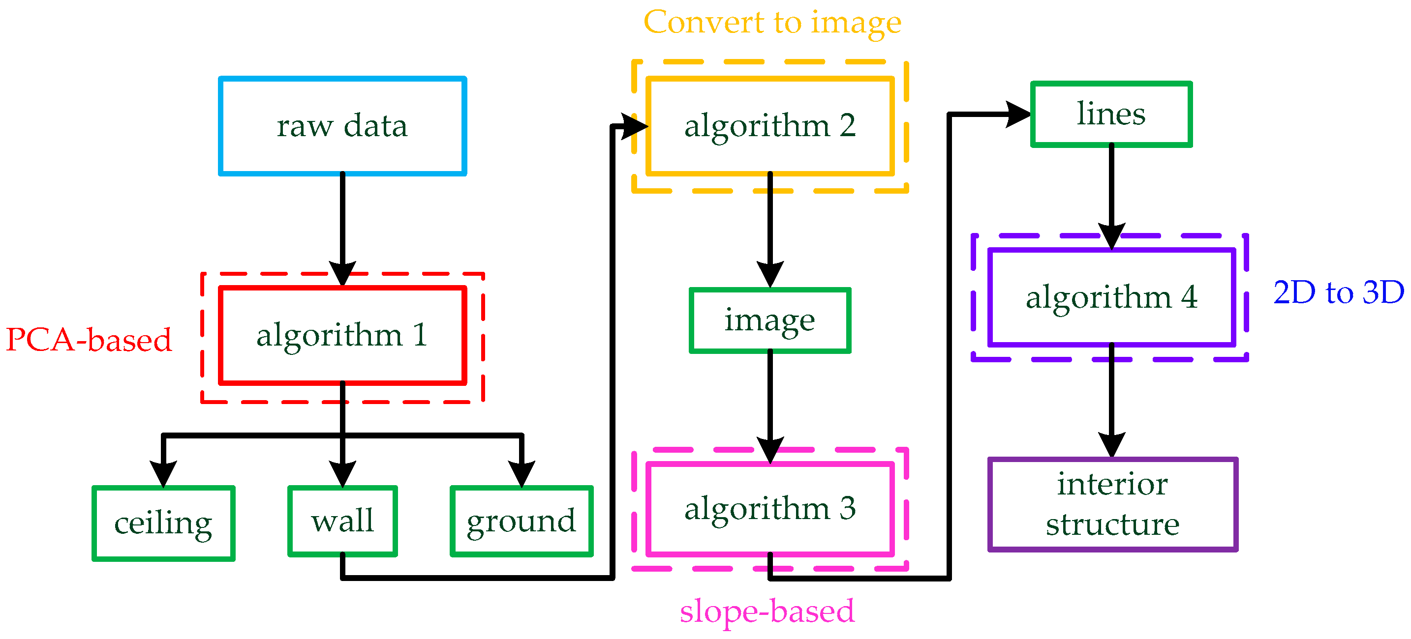
In general, the direct processing of point clouds is time consuming but robust, while dimensionality reduction or image conversion is fast but will reduce accuracy. To inherit the advantages of the above methods and make up for their shortcomings, we present our ideas in this paragraph. In this work, we propose a hypothesis: the walls are perpendicular to the ground and the angles between the walls are only within 0°, 45°, 90°, and 135°. To reduce time consumption, our data are collected by LiDAR because our target scene is relatively large. In previous studies, it is usually taken as a prior condition that the ground is the x-y plane. Based on a large number of experiments, we find that the prior condition is sometimes untenable. Therefore, we propose a PCA-based framework to find the floor and ceiling plane equations. Then, we project the complete wall onto the ground in the previous step and convert it into images rather than slicing. To remove the sparse noise and improve the filtering speed, we optimize the radius filtering without changing the effect. Next, coordinates are enlarged and meshed to convert them into pixels. After conversion to an image, the width of the line is several pixels, which is not conducive for us to extract the structure, so we consider extracting the image skeleton using the thinning algorithm. Saeed et al. [44] proposed an image-thinning algorithm that can extract image skeletons effectively; however, this algorithm is not sensitive to corner points. Zhang and Suen [45] proposed a method that could quickly and accurately extract an image skeleton and reflect image corner information by setting several constraint conditions through the relationship between the target pixel and eight-neighborhood pixels. Therefore, the method [43] is more suitable for our data. Due to the error in scan registration, the intersection of two lines produces a radian instead of a right angle. Corner detection in our data is difficult with traditional corner detection operators such as the Harris operator [46] and the SUSAN operator [47]. Chen et al. [48] proposed to use the curvature of each point as a constraint to screen corner points, which could not find corner points very accurately. By observation, we find that the intersection of adjacent lines can be used as the exact value of corner points. As such, we propose a judgment method of a straight line based on slope and select corners from the intersection points of straight lines. Finally, we restore the three-dimensional model according to corner points and corresponding lines. The entire flowchart is shown in Figure 1.
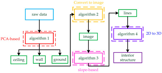
Figure 1.
The whole process of the method. The raw data are input to the PCA-based Algorithm 1, and the data are divided into three parts: ceiling, wall, and ground. Then, the three-dimensional wall is transformed into an image by Algorithm 2. Next, we use slope-based Algorithm 3 to find lines in the image. Finally, the three-dimensional interior structure is restored from lines by Algorithm 4.
The rest of this paper is organized as follows. Section 2.1 presents the principle of PCA and the framework that separates the walls based on PCA. In Section 2.2, we introduce how we can transform data into images, including point cloud projection, improved radius filtering, and data regularization. Section 2.3 presents the principle of the slope-based algorithm and some detailed processing and optimization. In Section 2.4, we organize the expression of straight lines and restore the three-dimensional structure of the interior environment. In Section 3.1, we introduce our equipment and the data extraction process. In Section 3.2, we use three different scenarios to verify our method and give the relevant evaluation parameters of three experimental results. Section 4 shows our discussion of the experimental results, including the advantages, disadvantages, and possible subsequent optimization of the experimental method. Finally, we summarize the whole paper and look ahead to future work in Section 5.
| Algorithm 1 Principal Component Analysis (PCA) |
| Input: |
| Output: |
| 1: |
| 2: for do |
| 3: |
| 4: end for |
| 5: |
| 6: |
| 7: |
| 8: |
| 9: |
| Algorithm 2 Wall extraction method |
| Input: |
| Output: |
| 1: |
| 2: |
| 3: |
| 4: |
| 5: |
| 6: for each grid do |
| 7: |
| 8: |
| 9: end for |
| 10: do SOR |
| 11: |
| 12: |
| 13: |
| 14: |
| Algorithm 3 Data format conversion method |
| Input: |
| Output: |
| 1: |
| 2: |
| 3: for do |
| 4: |
| 5: end for |
| 6: |
| 7: for do |
| 8: |
| 9: end for |
| 10: |
| 11: for do |
| 12: |
| 13: end for |
| 14: |
| 15: |
| 16: |
| 17: for do |
| 18: |
| 19: end for |
| Algorithm 4 Line segment extraction method |
| Input: |
| Output: |
| 1: |
| 2: for do |
| 3: |
| 4: |
| 5: end for |
| 6: |
| 7. for |
| 8: |
| 9: |
| 10: |
| 11: end for |
| 12: if |
| 13: |
| 14: end if |
| 15: for |
| 16: if |
| 17: |
| 18: end if |
| 19: for |
| 20: |
| 21: |
| 22: |
| 23: end for |
| 24: end for |
| 25: for |
| 26: |
| 27: if |
| 28: |
| 29: end if |
| 30: end for |
| 31: for |
| 32: |
| 33: |
| 34: |
| 35: end for |
| 36: |
2. Methods
In this section, we detail the principle of our approach in four steps: (1) A wall extraction method based on PCA; the data are divided into three sections: floor, ceiling, and other data. (2) Conversion from 3D to 2D data, including projection, filtering, and voxelization. (3) Extraction of line segments based on the image; the image is skeletonized and we propose a line segment-extraction algorithm based on the slope of adjacent points. (4) Reconstruction of the indoor structure; we reconstruct the interior structure using linear information.
2.1. Extraction of Wall Based on PCA
PCA can be used to extract the principal components of data, reduce the dimensionality of data, or fit planes or lines. In this section, we use the theory of PCA to find the floor and ceiling of the data and solve the problem that the floor may not be the x-y plane in the x-y-z frame.
The principle of PCA is shown in Algorithm 1. The input is the three-dimensional point cloud. Then, the average of the point clouds is calculated. For the point , the deviation of and is calculated, and the deviation matrix consists of . Next, the covariance matrix is calculated by and we obtain the transformation matrix by singular value decomposition (SVD). and are taken as vectors of the fitting plane, and is taken as a normal vector to that plane. Finally, we project the raw 3D data to obtain the 2D data by matrix operation .
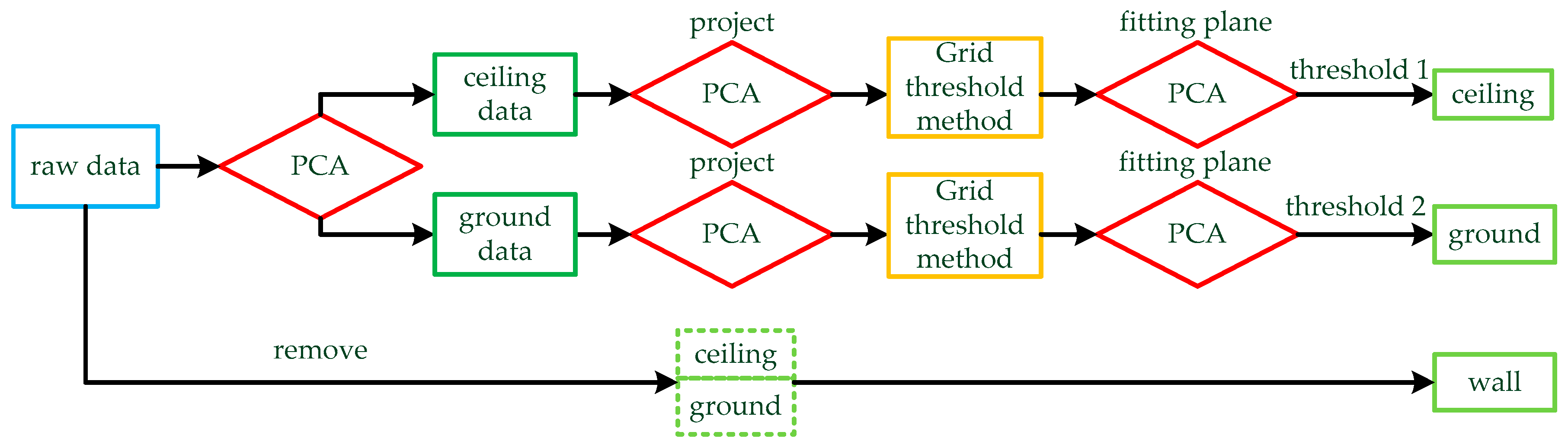
Our first step is the process of finding the plane based on PCA. The main flow of this method is shown in Figure 2 and Algorithm 2. is used as the raw data for Algorithm 2.
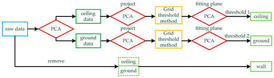
Figure 2.
Wall extraction method based on PCA: PCA is used to fit the plane for the raw data, and the data are divided into two parts by the plane: ceiling data and ground data. The two parts of data are projected into two-dimensional data by PCA, and then the grid threshold method is used to find the feature points of the ground and ceiling. PCA is used to fit the feature points to obtain the level of the ground and ceiling. Finally, thresholds are set for the two planes and the point clouds of the floor and ceiling are removed.
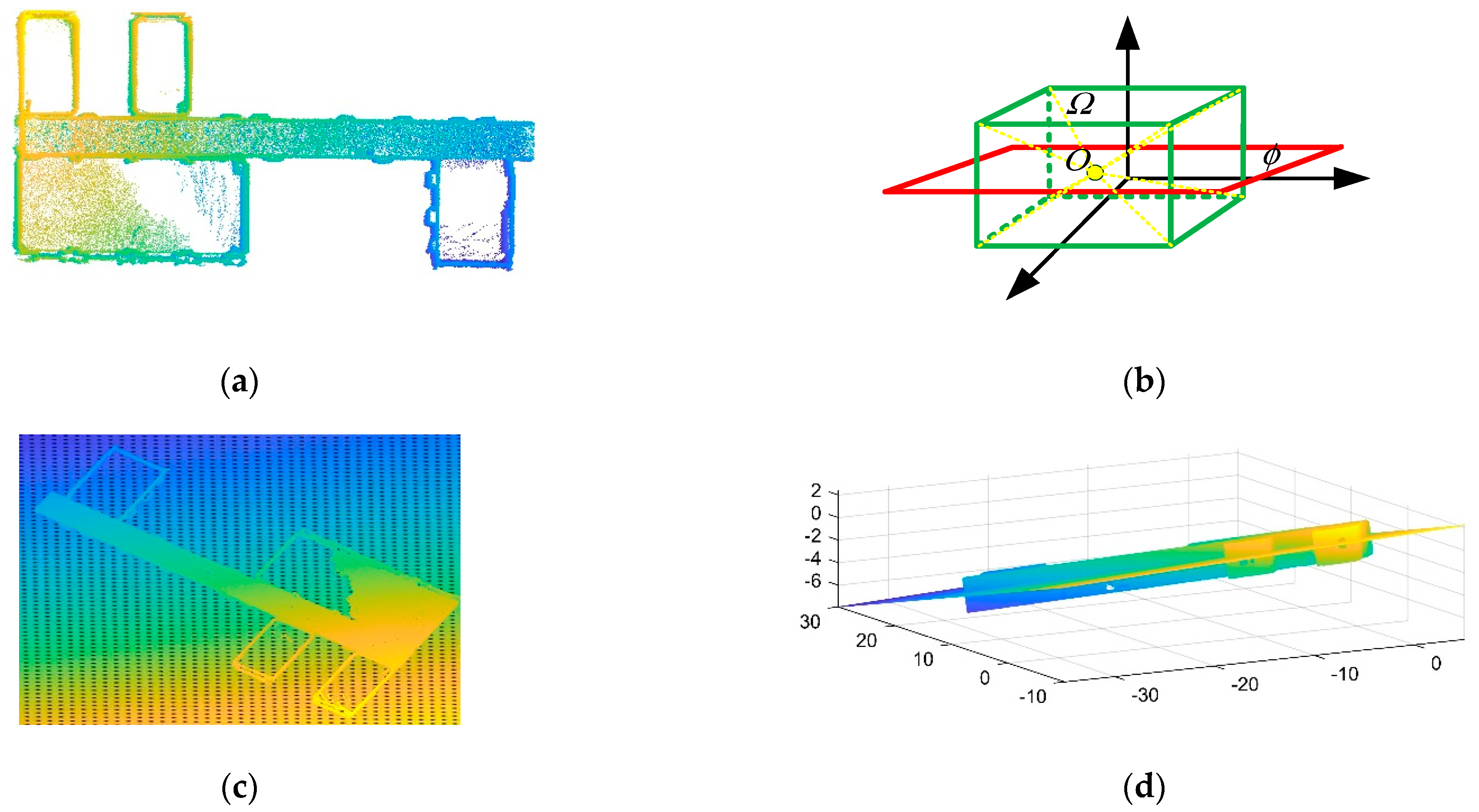
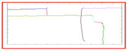
is used as the raw data in Algorithm 2. To better represent the effect of the algorithm, we use test data to verify our algorithm, as shown in Figure 3a. The sum of the distances of all points from the plane is minimum by fitting regular data as follows:

Figure 3.
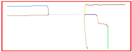
PCA is used to find cross-sections of the data: (a) raw point cloud data; (b) suppose that is a cuboid composed of point clouds and is the average value of data; is the plane determined by the normal vector and obtained from PCA; (c,d) the plane fitted in the raw data by PCA.
Therefore, the plane fitted by the symmetric point cloud is in the middle of the data, as shown in Figure 3b. Due to indoor noise and other objects, the position of the plane is changed, but the data are also divided into upper and lower parts. The upper part contains the ceiling and the lower part contains the floor, as shown in Figure 3c,d.
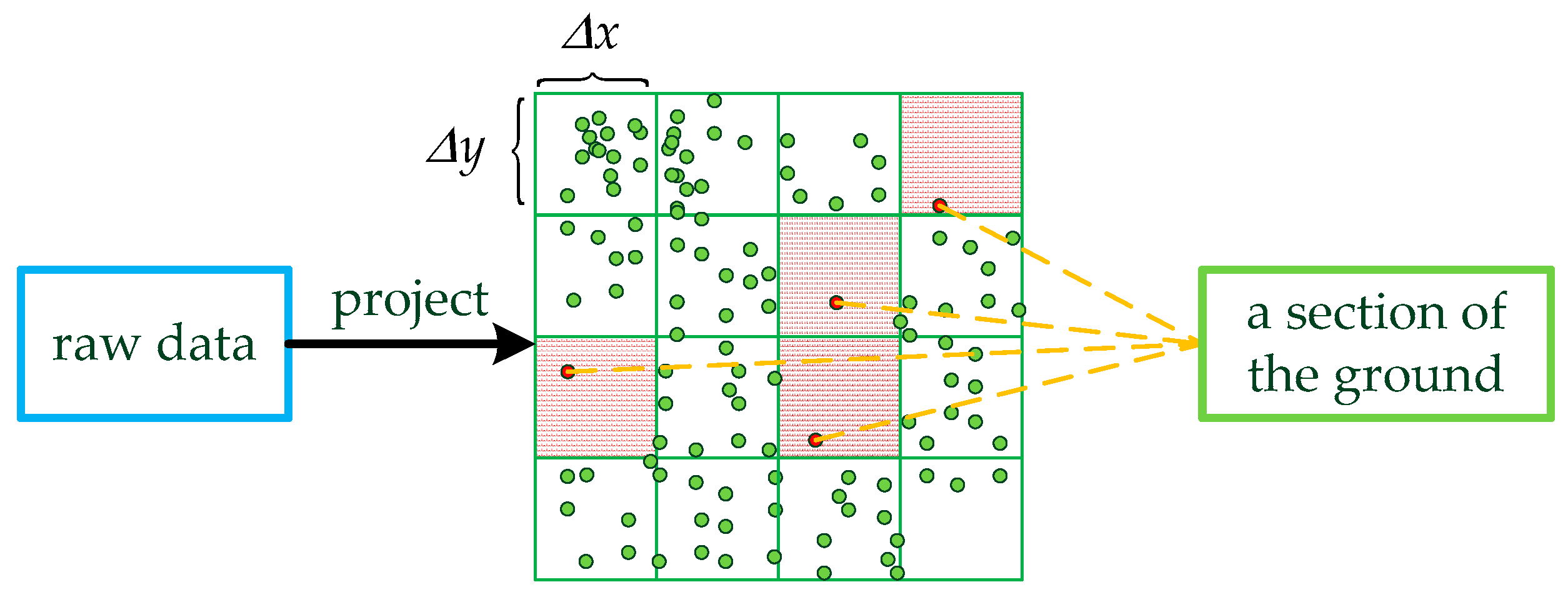
Then, and are projected on planes and converted into two-dimensional and . and are processed by the grid threshold method and we introduce the method using as an example. The method is shown in Figure 4.
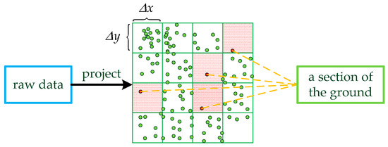
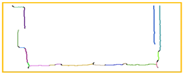
Figure 4.
The grid threshold method. The original data are projected two-dimensionally and meshed. Part of the ground data consists of these points whose quantity is one in the grid.
We set the number of grids, and then calculate the horizontal resolution and vertical resolution of the grid according to the maximum values and of in two directions as follows:
Points in the same grid are assigned the same number:
Some edge problems are caused by rounding the number of points. Therefore, we take some measures as follows:
For the number of each point, we replace 0 with 1 and replace the points that are larger than with . The data whose number corresponds to one point are taken as the plane points. However, due to the interference of noise, we use the SOR filter to obtain the exact plane points. These points are fitted into a plane by PCA, and and correspond to the plane:
Since the ceiling and floor are parallel, we take the average of the normal vectors of the two planes as our new normal vector:
Finally, we set and of the distance from the point to the planes to determine the ceiling and the floor , and the wall is the data except for and . The entire process is shown in Table 1.

Table 1.
The process of extracting the wall: Project the initial data onto a plane, and then the ground data are screened by the grid threshold method. The ground is restored to a three-dimensional form and treated with the SOR filter. The ground and ceiling are fitted into a plane; then, the wall data are extracted by setting thresholds.
2.2. Data Format Conversion
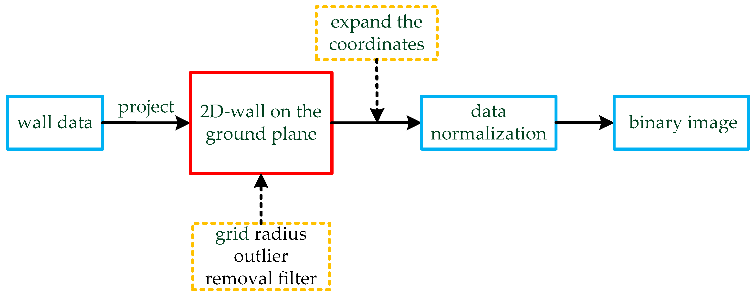
The point cloud data are so dense and disordered that it is difficult to extract information from them. However, point cloud slicing leads to the loss of the contour, which increases the difficulty of subsequent processing. Therefore, to improve the efficiency of the algorithm, we projected the wall onto the ground and meshed it. The entire process is shown in Figure 5 and Algorithm 3.

Figure 5.
The process of data conversion. The wall data are projected on the ground plane, which was fitted in the previous section. The two-dimensional data are processed by a grid radius outlier removal (GROR) filter, and the coordinate values are enlarged by appropriate multiples. Finally, the data are normalized and transformed into a binary image.
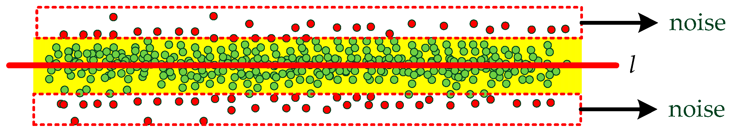
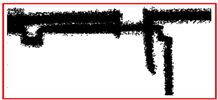
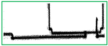
is used as the raw data in Algorithm 3, and is projected into on the ground plane. Due to the influence of noise, the points of a line have a certain width, and we extract the line features from these points. First, we need to remove the noise of the two-dimensional points, as shown in Figure 6.
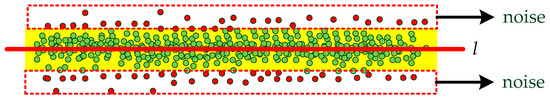
Figure 6.
The noise in the points. We need to extract the line and remove the noise.
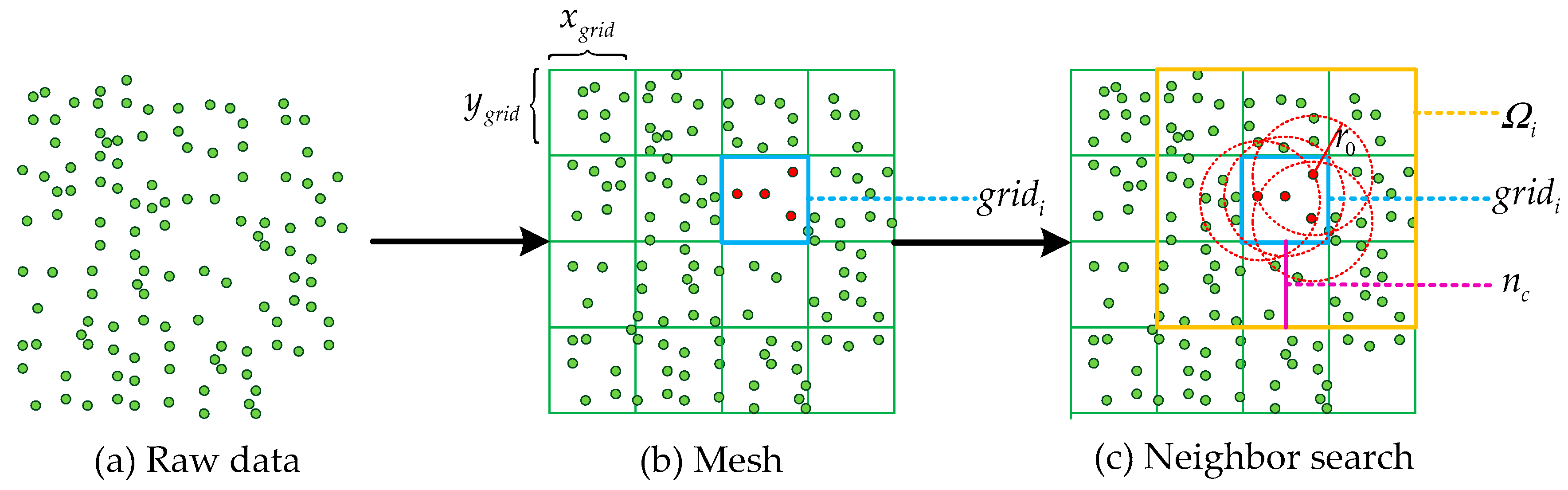
The radius outlier removal (ROR) [49] filter is an effective tool for noise removal. If the ROR filter is not optimized in any way, this method is very inefficient. Therefore, we use the GROR (grid radius outlier removal) filter to optimize the ROR filter. We mesh the data and then search for the nearest neighbor points in a specific way. The results show that the efficiency of this method is greatly improved without affecting the accuracy of the ROR filter. At the same time, due to the high density of the vertical wall point and the low density of other sundries points after projection, some sundries points are removed by the GROR filter. The principle of this method is shown in Figure 7.
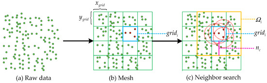
Figure 7.
Grid radius outlier removal (GROR) filter. The resolutions of the divided grid are and . The grid to be processed is . is the number of adjacent grids, and the search area is determined by . is the radius of the neighbor search.
First, the raw data are divided into grids, and the resolutions in the two directions are, respectively, and . The points in each grid are searched for their nearest neighbors. If only the points in the grid are used as the search scope, some of the nearest neighbors will be lost at the edge of the grid. Therefore, we have expanded the area to ensure the accuracy of the search. For the grid , we use the number of adjacent grids to expand the region. is determined by the search radius and resolutions:
The radius divided by the minimum resolution and ceiled is called . Therefore, the search area for the grid is as follows:
Since the mesh size is fixed, edge suppression is added as follows:
Finally, the points whose number of neighbors is less than are removed. After removing the noise, we need to expand the coordinates of the points . We chose a large multiple to make the details of the data more obvious as follows:
For each point , we subtract the minimum value of the point to make sure the points are positive and use the multiple to expand the coordinate of these points. Since the coordinates need to be rounded after expanding, and then restored after processing, the details can be better reflected and the error can be reduced by a larger multiple. Assume a point is , and when it expands 100 times it becomes . We round it to and then restore it to . The error before and after treatment was less than 0.01.
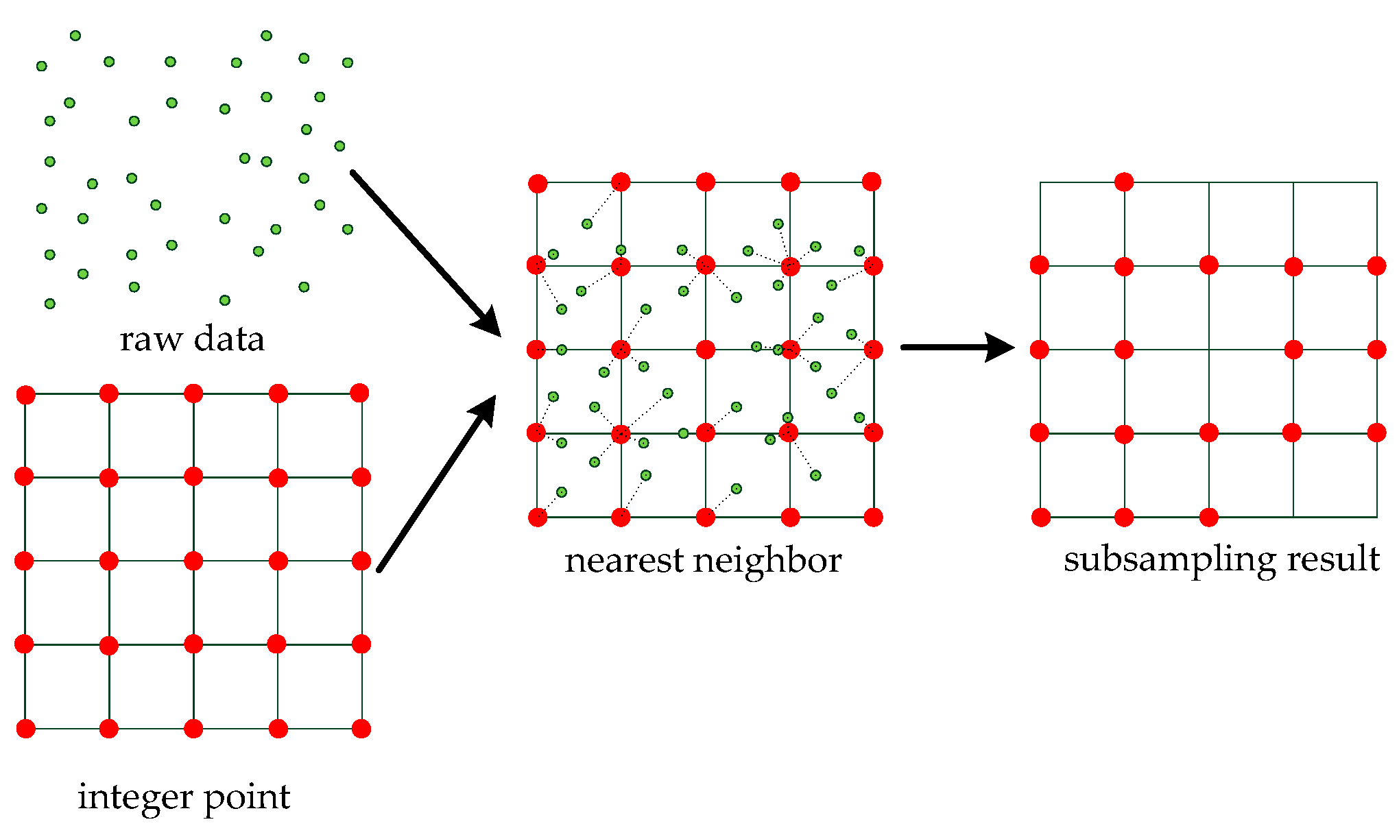
Then, we use the grid subsampling method to round the coordinates and eliminate the repeated coordinates of the same position. The benefit of this method is that the data become regular and the amount of data is greatly reduced. The principle of the method is shown in Figure 8.
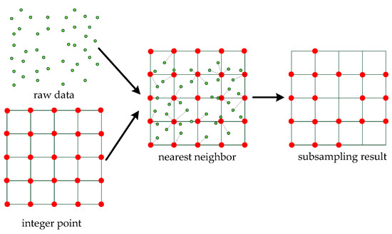
Figure 8.
The grid subsampling method. Given the coordinates of integer points, each point in the raw data is updated to the nearest integer point. The shape of the data is retained and the amount of data is reduced in the subsampling result .
For the raw data and integer points , is replaced by the point nearest to . Then, the overlapping points are removed. Finally, we obtain the data after the subsampling. For each point , we need to replace 0 with 1 as follows:
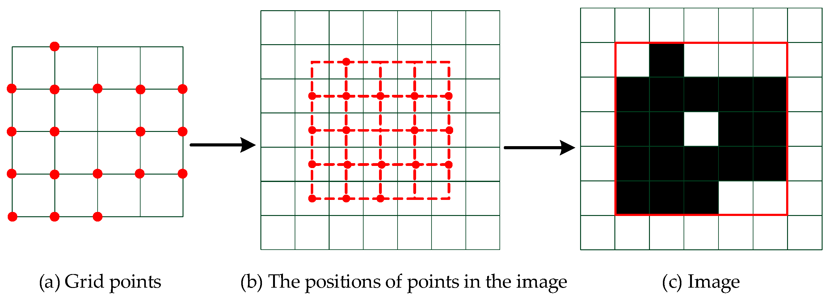
Since the coordinates of the data are all positive integers, the data can be converted into images to prepare for the next step. This process is shown in Figure 9. The size of the image is determined by the maximum value of the coordinates in the two directions of the point as follows:
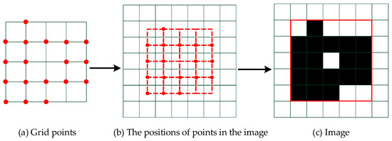
Figure 9.
The process of converting grid points to the image: the pixel corresponding to the positions of the grid points in the image is given the value . The image is made up of pixels in the red box in the final step.
Additionally, the pixel of the position corresponding to in the image is replaced by :
where the parameter is against the background; for example, the parameter is 0 and the background is 1 in the image.
Therefore, we obtain two sets of data: the two-dimensional points with a grid structure and the corresponding images of the two-dimensional points. The shape of the raw data is retained and the scattered points are regularized by the two data. The experimental procedure in this section is shown in Table 2.
Table 2.
Projection and transformation of data. First, the raw data are projected onto the ground plane. Then, the noise is removed by the GROR filter. We enlarge the coordinates 70 times and the grid subsampling method is used to make the data regular. The regular data can be converted to an image, which is prepared for the next section.
2.3. Extraction of Line Segments
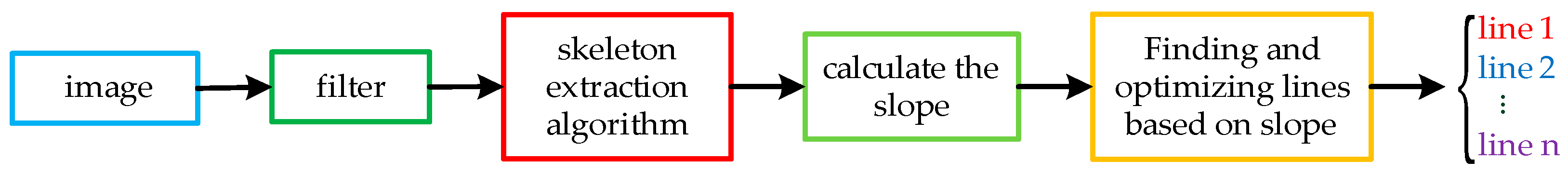
For the image in the previous section, we need to extract line segment information from it. Since straight lines are composed of points with a certain thickness in the data, it is difficult to extract multiple lines directly from the data. Therefore, we first use the thinning algorithm to extract the skeleton of the image. Then, the corresponding slope of each point is calculated based on the nearest neighbor point. Finally, we propose a slope-based search method to extract the line segments. We give the flow of the algorithm as shown in Figure 10 and Algorithm 4.

Figure 10.
The process of line segment extraction. First, filtering is used to remove the burrs from the image, and existing skeleton extraction algorithms are used to extract the image algorithm. Then, we calculate the slopes of the points and optimize the slopes accordingly. Finally, we judge all lines according to the specified rules.
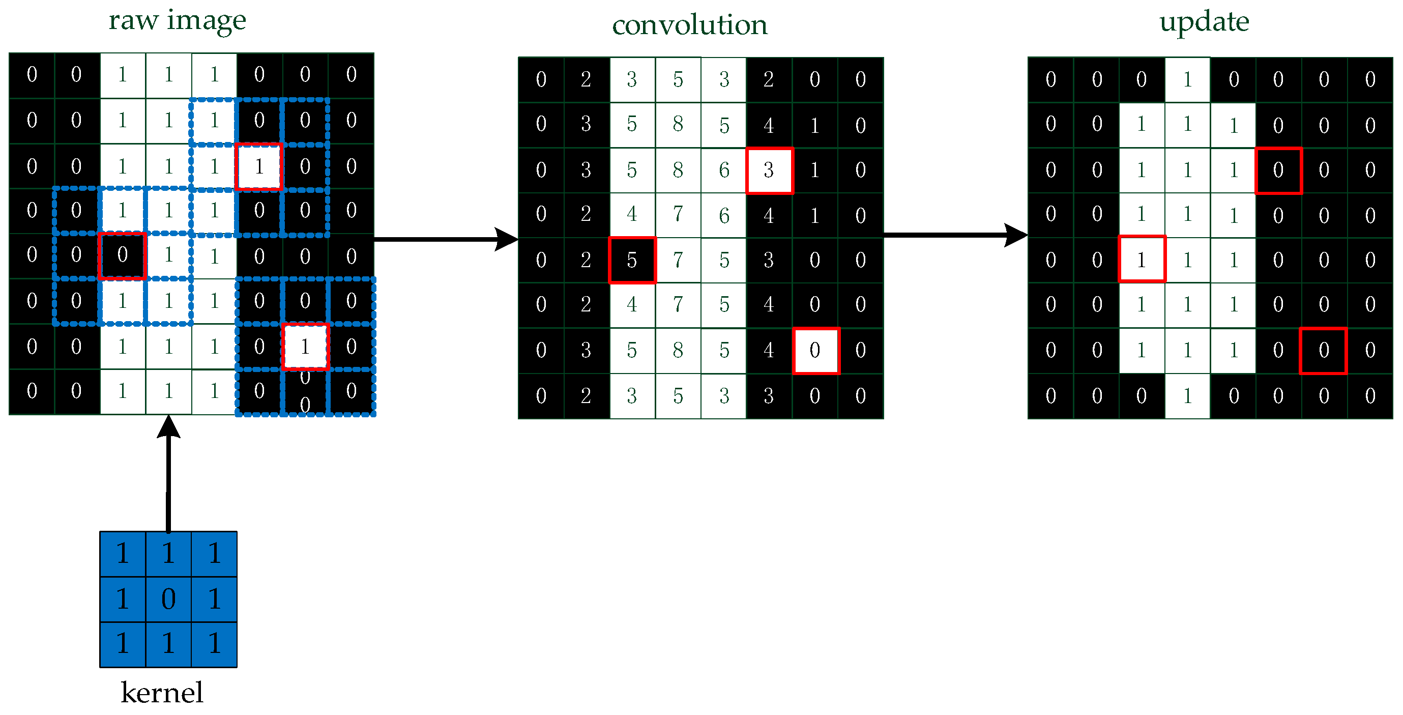
The image is the input in Algorithm 4. We assume that the background is 0 and the points are 1 in the image, and we convolve the image with a kernel to remove the burr, which is influential in extracting the skeleton. Then, the image is updated by the convolution value :
The pixel value is updated by comparing the convolution value with the number 4, as shown in Figure 11.

Figure 11.
A simple method to remove the burr. We convolve the image and update the pixels of the image based on the convolution values.
To better reflect the contour features of the wall, we consider refining the image. If the pixel representing the line is refined into a single pixel, the feature of the line is more obvious in the skeleton. Therefore, we use a suitable thinning algorithm to extract the two-dimensional skeleton information of the wall through experiments. The results are shown in Table 3.
Table 3.
Image skeleton extraction. The contour of the image is extracted by the skeleton extraction algorithm and lines are refined into single pixels. Similarly, the skeleton made up of two-dimensional points is reduced by the image skeleton.
The image skeleton is a single-pixel structure; we find that the characteristics of the lines are obvious, and the corners of the data affected by the error have a certain radian. Therefore, it is very difficult to extract the exact corners from the data; thus, we consider extracting the lines and determining the corners from the lines. We propose a line extraction method based on the nearest neighbor slope, and then introduce this method in detail.
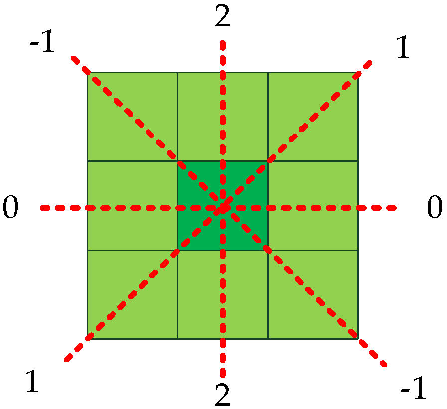
First, the random point is the starting point; its nearest neighbor is found and the slope of the two points is calculated. In this section, the neighbor points are all found in the 8 neighborhoods. If there are multiple nearest neighbor points, select one as the nearest neighbor point at random. Then, their slope is calculated as follows:
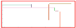
The slope of these two points is represented by the slope . Since the pixel positions in the image are all integers, there are only four cases for the slope of two adjacent points: 0, 1, −1, and the slope that does not exist is replaced by 2, as shown in Figure 12.
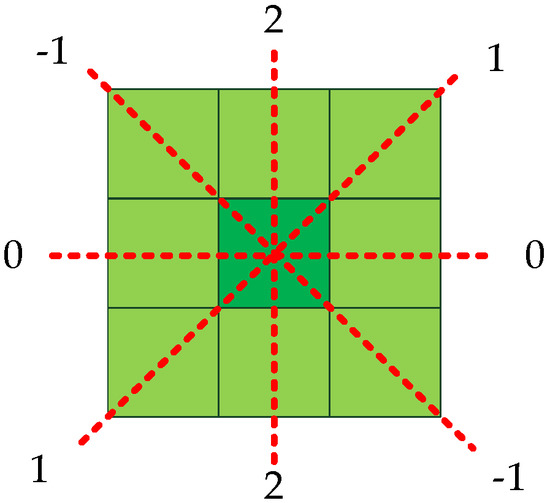
Figure 12.
The slope of the nearest neighbor. The slope is given four values: 0, 1, −1, 2.
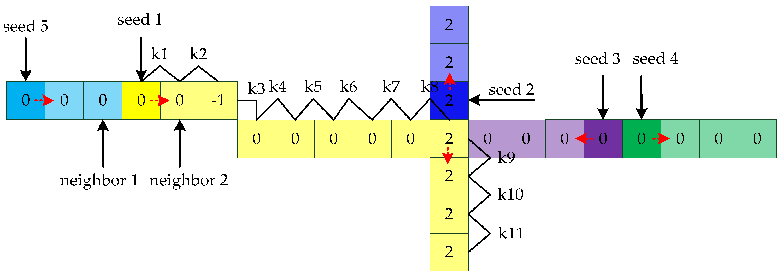
Then, the point is the next seed and its nearest neighbor is found to calculate the next slope, and the points whose slopes have already been calculated are not considered next neighbor search objects. The starting point is randomly selected until the seed point has no neighbors. If the slopes of all points are calculated, the algorithm stops. The process of calculating the slopes is shown in Figure 13.

Figure 13.
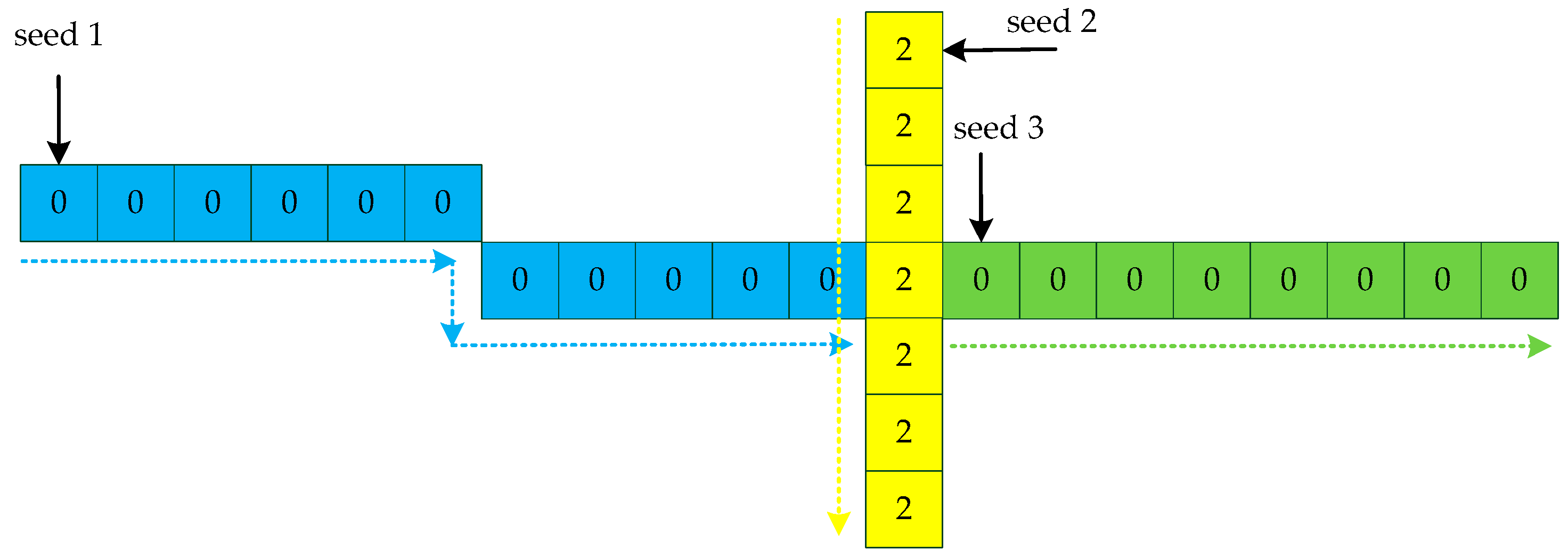
The process of calculating the slope. First, seed 1 is randomly selected in the image. Seed 1 has multiple nearest neighbor points and picks one at random to calculate the slope value 0. The values of seed 1 and neighbor 2 are 0. Then, neighbor 2 is the next seed 1. The points for which the slope has been calculated are not searched later. Seed 1 stops growing if the current point has no neighbors. Then, seed n is randomly selected and the same growth process is carried out until all the pixels of the image are calculated.
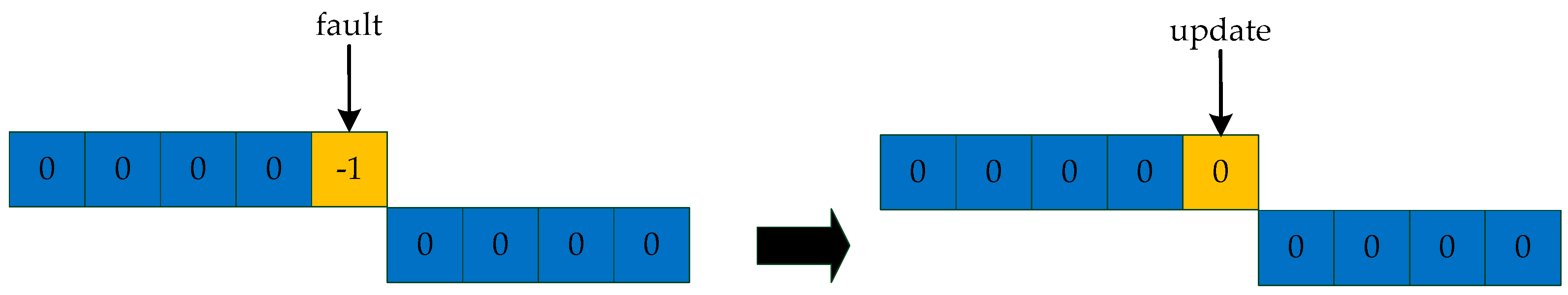
After calculating the slope at all points, we need to eliminate the fault in the line, as shown in Figure 14. For each point, if it only has two neighbors and the two neighbors have the same slope , update the slope of that point to .
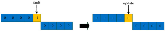
Figure 14.
Eliminate faults in lines. The fault is caused by noise and algorithm error, and we update the slope of the current point using the slope of the point’s nearest neighbor.
When the slope of all the points is calculated, we look for lines based on the slope. The idea is to start at one endpoint of each line as a seed point and grow until the line is completely extracted. Therefore, we first need to look for endpoints as seed points. We use the following three conditions to determine the seed point : (1) the number of neighbors is two and the slopes of the neighbors are satisfied with ; (2) the number of neighbors is one; (3) no neighbors. The point that satisfies any of these conditions is considered a seed. Next, we extract points on the same line from the seed, as shown in Figure 15. For a straight line, look for a point within the 8 neighborhoods of the seed that has the same slope as the seed. In these data, the number of the point is only 1 or 0. If the number is 1, the point is the next new seed, and the raw point is removed. If the number is 0, the points we calculated before form a line. Keep picking seed points until all the points are divided into lines.

Figure 15.
Line searching method based on slopes. Determine the seed point according to the judgment condition, and then find the line according to the slope of the nearest neighbor point until traversing all the points.
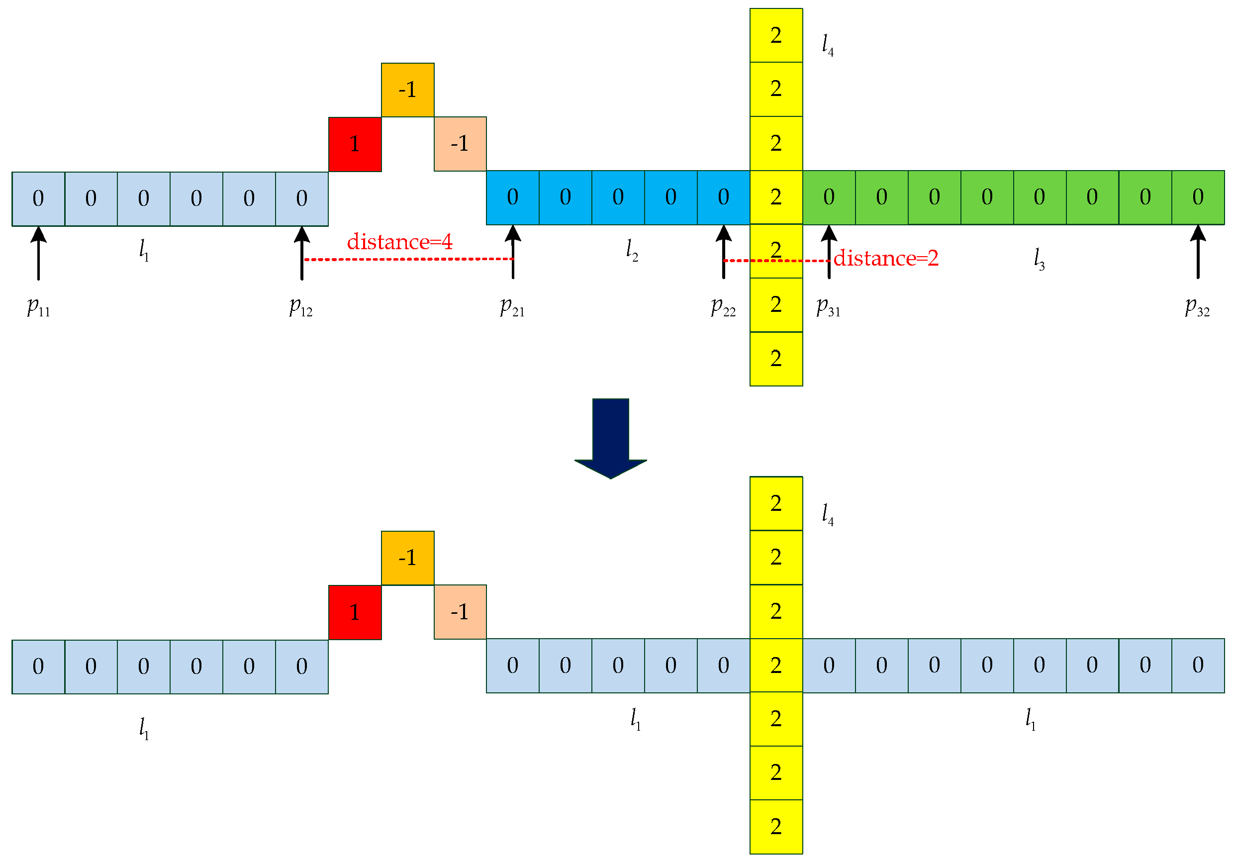
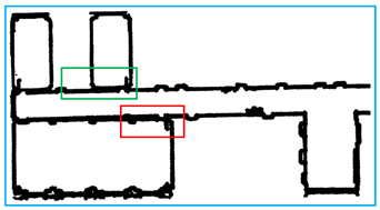
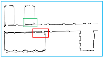
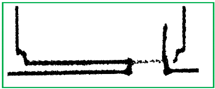
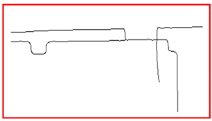
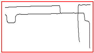
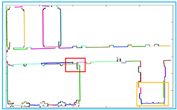
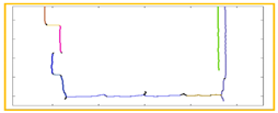
When all the lines are categorized, we need to set thresholds to eliminate non-line points. Due to our conditions applied to individual points and short line segments, lines containing fewer points are removed. Since the same line is divided into sections by noise, we propose a method to solve this problem. As shown in Figure 16, for two endpoints of each line, two lines are the same line only if the distance of two endpoints is less than the threshold and the two lines have the same slope. For the line , we compare the line to the lines , then compare the line to the lines , until, finally, we compare the line to the line . When all lines have been identified, repeat the steps until the number of lines is changeless.
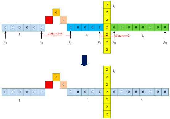
Figure 16.
An example for updating lines. We set the distance threshold to 5. For the line and the line , the distance between the endpoint and the endpoint is less than the threshold. Therefore, the two lines are classified as the same line. In the same way, the line and the line are classified as the same line.
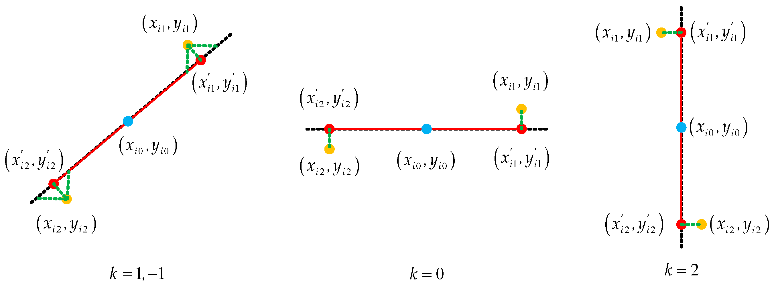
For these lines, due to the points that make them up not being in a line, we need to figure out their slopes and endpoints to update the lines. The principle of updating the endpoints is shown in Figure 17. We know the parameter of the line : two endpoints , midpoint , and slope . If the slope is 1 or −1, we can obtain new endpoints based on these parameters as follows:
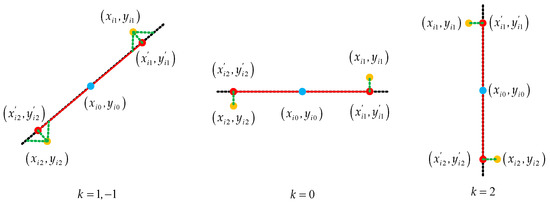
Figure 17.
The process of determining new endpoints. The dotted line is defined by the midpoint and the slope . If the slope is 1 or −1, the vertical point of the raw endpoints on the line is the new endpoint. We calculate the points in which the original endpoint intersects the line in both the horizontal and vertical directions; the midpoint of the points is a new endpoint. If the slope is 0, the abscissa of the new endpoints is the same as the raw endpoints, and the ordinate is the same as the midpoint. If the slope is 2, the abscissa of the new endpoints is the same as the midpoint, and the ordinate is the same as the raw endpoints.
If the slope is 0, we obtain new endpoints as follows:
If the slope is 2, we obtain new endpoints as follows:
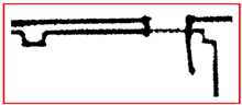
Therefore, the line is determined by the midpoint and the slope, and the range of the line is determined by the new endpoints. Finally, we show the process of finding the straight lines and drawing them all, as shown in Table 4.
Table 4.
The process of finding lines. In these images, each line segment is represented by a separate color except black. First, we find points that belong to the same line by using neighboring points. In detail, we can see that points that originally belong to the same line are divided into multiple lines due to noise and algorithm. Then, by optimizing the line based on endpoint and slope, we solve the problem. Finally, we draw the lines by slope, midpoint, and new endpoints.
2.4. Structure Reconstruction
In this part, we optimize the lines and reduce them to three-dimensional planes. In the last section, due to the error of scan registration, we removed the smooth intersection of the adjacent segments. Therefore, we propose a method to connect the lines. The basic steps of this method are as follows:
- Assuming that the known condition is the endpoint , the nearest endpoint of the other lines is calculated. Additionally, we then calculate the distance between the two endpoints.
- The distance threshold is set to avoid two lines that are far apart from each other being connected. Then, we compare the distance to the threshold.
- If the distance is less than the threshold and the two lines are perpendicular, the lines corresponding to the two endpoints are connected and the endpoints and are replaced by the intersection. For the slopes and of the two lines, we think these two lines are perpendicular if they satisfy the condition:
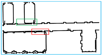
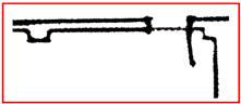
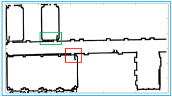
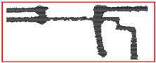
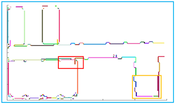
The results are shown in Figure 18. To better demonstrate the accuracy of the experimental results, we spliced and compared the lines with the raw data, as shown in Figure 19.
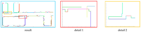
Figure 18.
The result of line correction. All the lines that satisfy the condition are connected and we show them in detail.
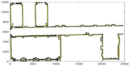
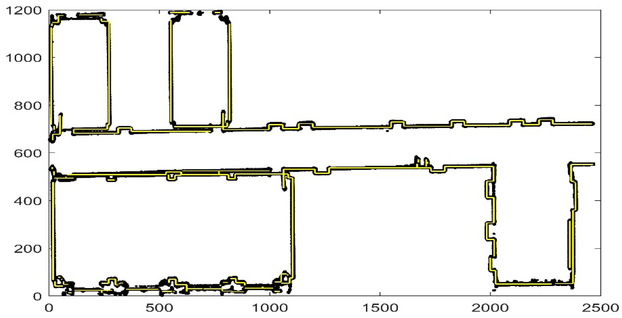
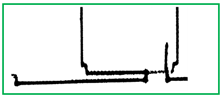
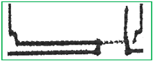
Figure 19.
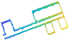
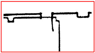
Comparison of experimental results. The yellow line is the result that we obtain and the black points are the raw data. We obtain the basic outline of the data, and the reason why some parts are not considered lines is that the points are discontinuous or the slope changes are complicated.
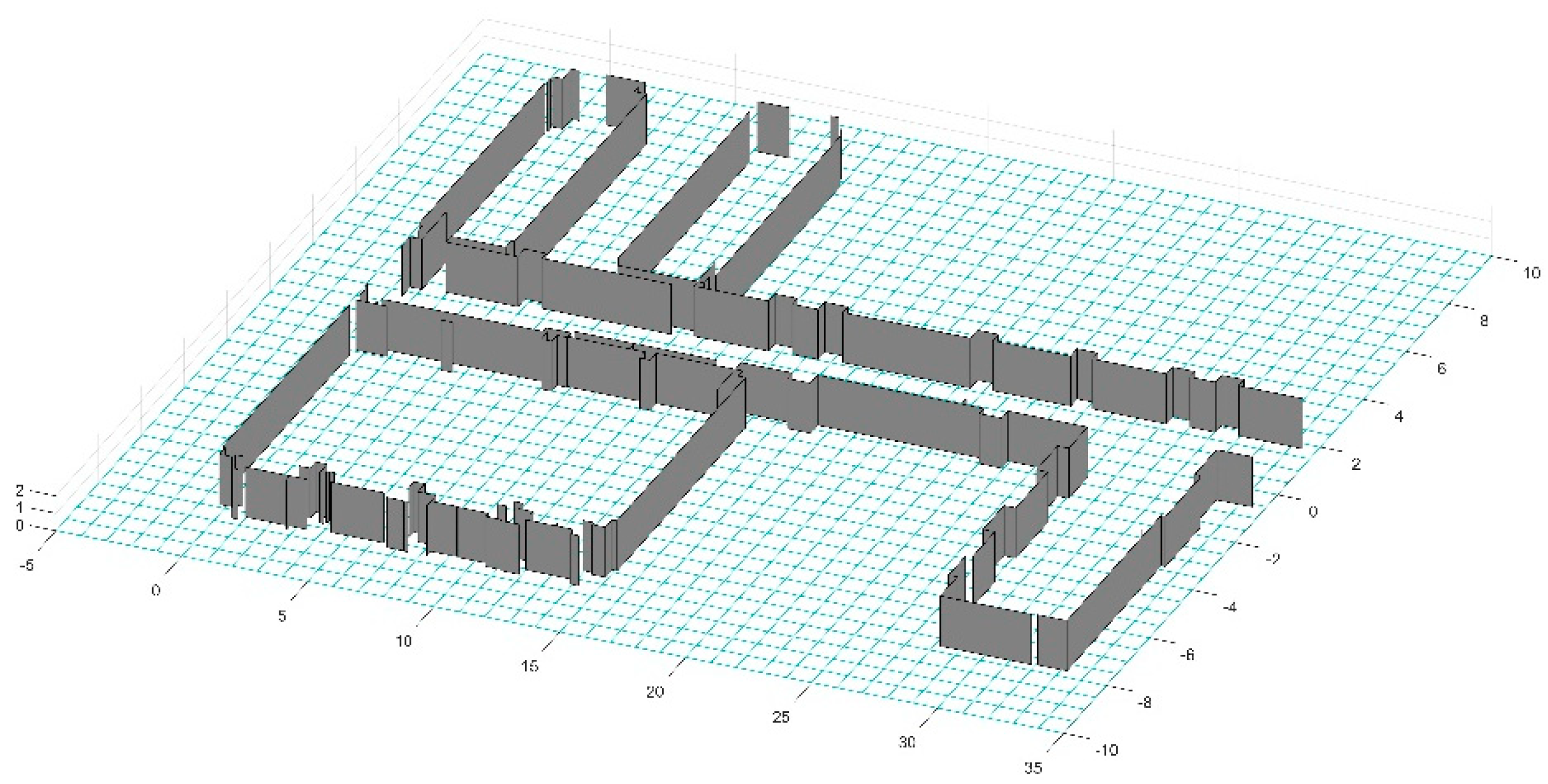
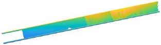
Finally, we reconstruct the three-dimensional plane from the resulting lines. Now, we need to figure out the height of each line. In the previous section, we calculated the ground plane and calculated the height of each point above the ground. Before we achieve this, the endpoints are restored by Equation (10). We calculate the nearest neighbors of the midpoints of each line segment and choose the height of the line as the maximum distance between these neighbors and the ground. If the height is close to the distance between the ceiling and the floor, the height changes to that distance. The result is shown in Figure 20. At this point, we have introduced the principle of the whole algorithm in detail. In the next section, we will evaluate the performance of the algorithm with multiple sets of data.
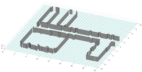
Figure 20.
The result of three-dimensional reconstruction. To make the result clearer, we removed the ceiling and painted all the vertical planes on the ground.
3. Experimental Results
3.1. Preparation of Experimental Data
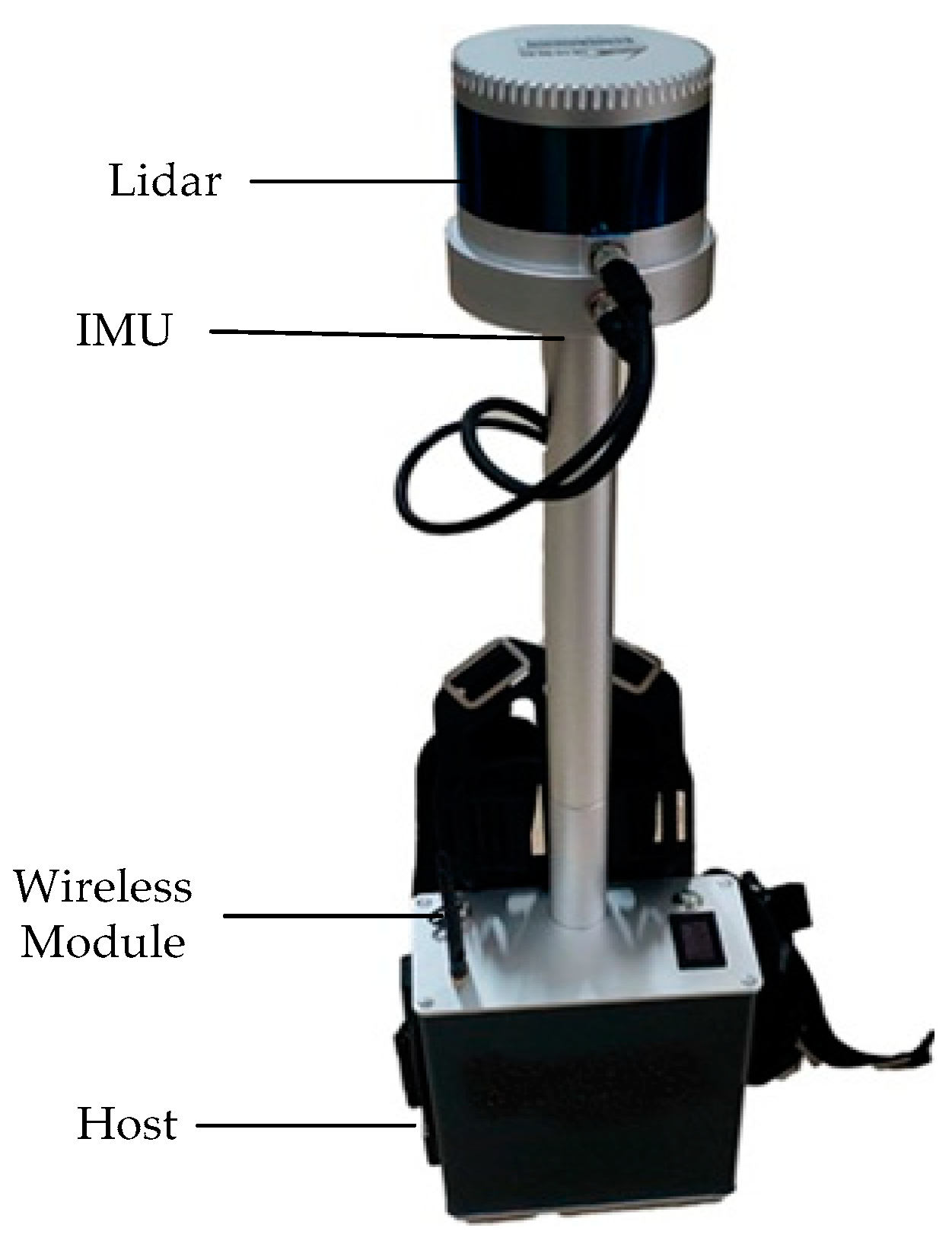
The equipment used to collect data is shown in Figure 21. The experimental equipment was a backpack system integrating LiDAR, an inertial measurement unit (IMU), a wireless module, and an upper computer. The surroundings are sensed by a 16-line mechanical LiDAR at a frequency of 0.5 s and surface information about surrounding objects is scanned by the LiDAR. The IMU is used to measure the attitude information of LiDAR and we fuse it with each frame point cloud by the robotic operating system (ROS) in the upper computer. The processed data are transmitted to a computer for display through the wireless module.

Figure 21.
The experimental equipment. It is a backpack system integrating LiDAR, an inertial measurement unit (IMU), a wireless module, and an upper computer.
We adopted LeGO-LOAM to implement the scan registration of data. In the algorithm, the attitude is obtained from the ground features, and the attitude is calculated according to the remaining point cloud features. Therefore, the matching error is caused by too few ground features, and another error is caused by the Euler angles turning too fast in a short time. In the following experimental results, these two aspects may be the causes of the error. Finally, we present some important parameters for the next three scenarios: the number of grids for the floor and ceiling is extracted in Section 2.1. Radius and threshold of the GROR filter, magnification of the coordinates, the distance that connects parallel lines, and the distance between the vertical lines are shown in Table 5.
Table 5.
Some important parameter settings for the scenarios.
3.2. Results
In this section, we use three real scenarios to test our algorithm. We carried the equipment on our backs and the LiDAR was about 1.8 m away from the ground. We followed a fixed trajectory and tried to keep the posture of the device stable as we moved. Finally, three data points are prepared: a room, a floor, and some rooms.
3.2.1. Experiment Scene 1
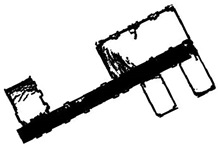
We extracted the structure of a single room in the first data point; the room was about 7.69 m 6.35 m 3 m (length width height). The experimental scene is shown in Figure 22a, and the two-dimensional plan of the scene is shown in Figure 22b. To better show the interior structure, we removed the ceiling in the second section. The measured point cloud data are shown in Figure 22c, and the final result is shown in Figure 22d.
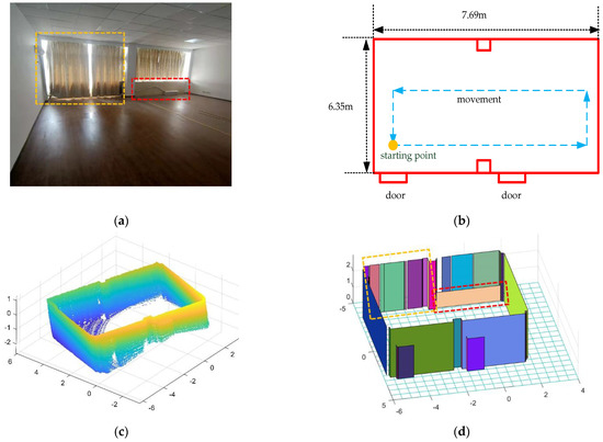
Figure 22.
The resulting presentation of scene 1: (a) photo of the real scene; (b) the two-dimensional plane of the scene; we measured the dimensions of the room and marked the starting point and trajectory; (c) point cloud data after removing the ceiling; (d) the result of the reconstruction of the interior structure, and each color represents a plane.
It can be seen from the experimental results that the basic structure of the room has been restored, but we can see that there are some flaws in the results. There are gaps between some adjacent planes. In the previous sections, we joined planes if they were adjacent and the distance between them was less than the threshold. In real scene 1, due to the glass between the curtains not being sensed by the LiDAR, we kept the gaps in the result. At the same time, the large gaps due to measurement errors were preserved.
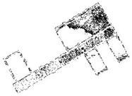
3.2.2. Experiment Scene 2
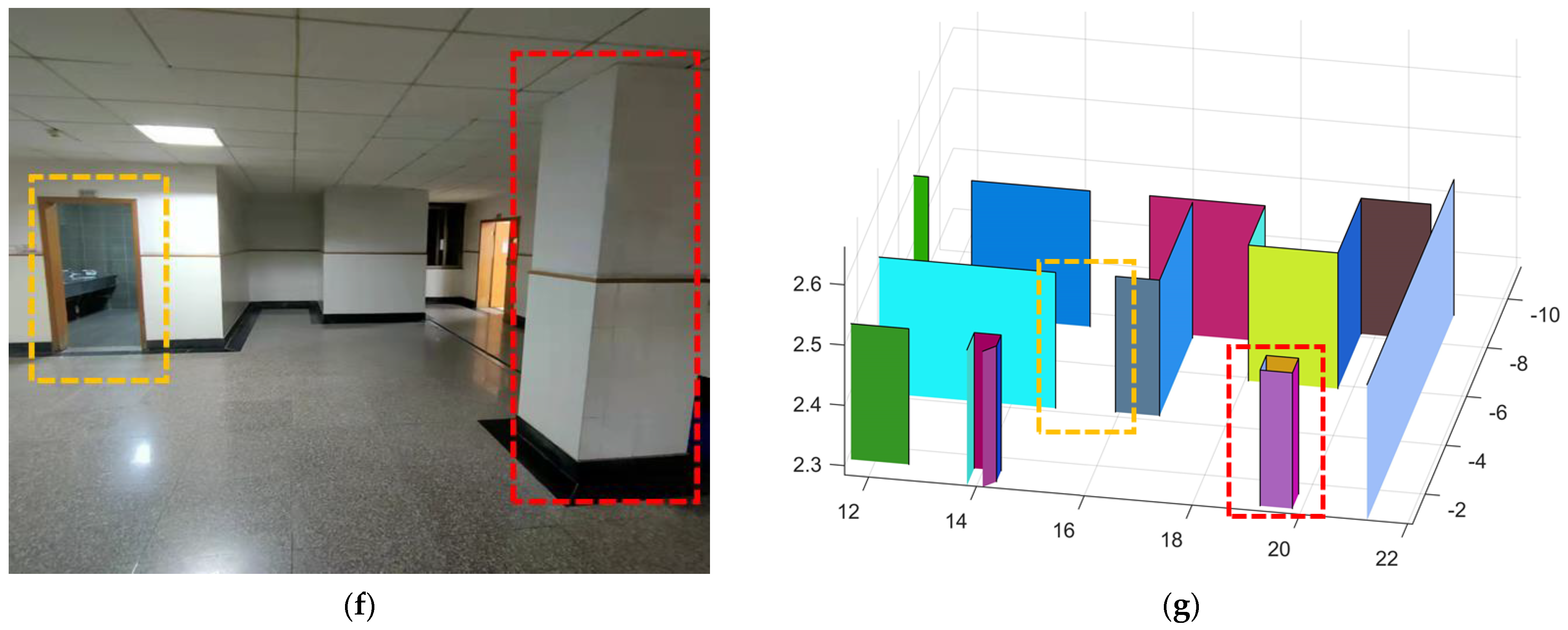
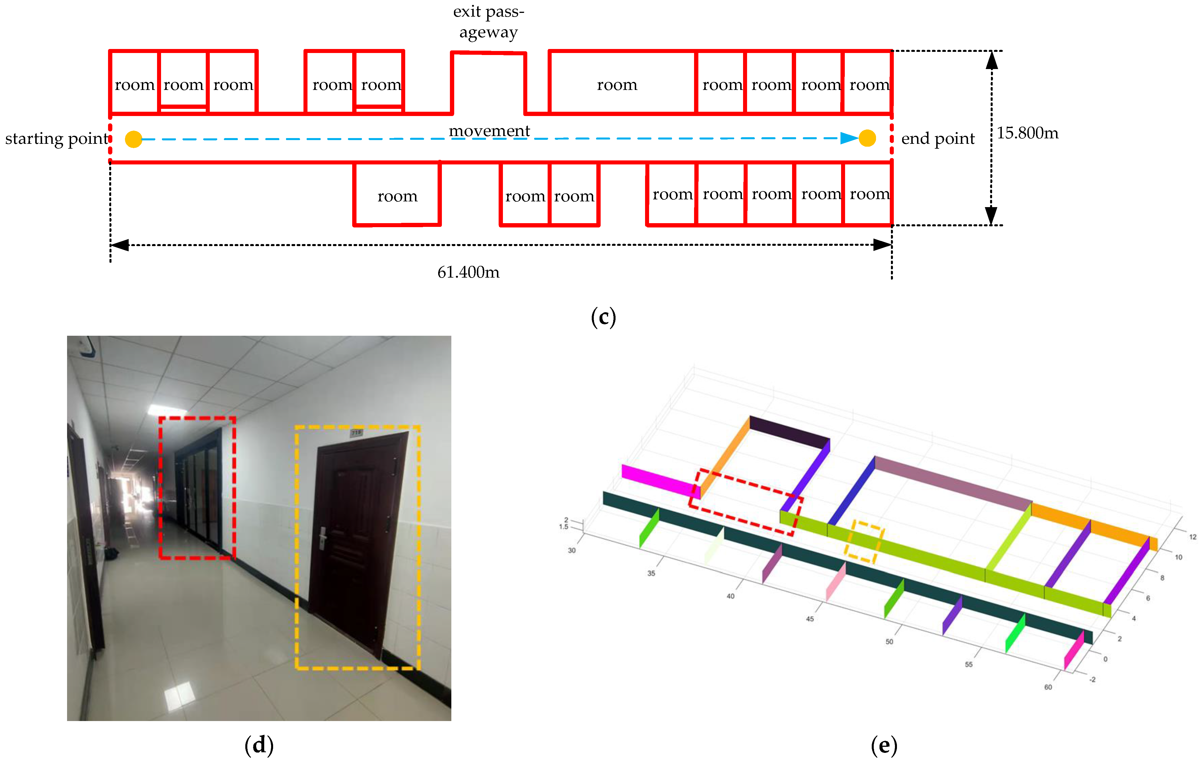
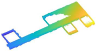
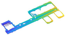
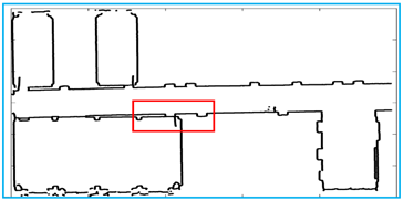
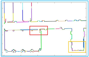
We chose the floor of the school building as the second scenario to test the method. The point cloud we collected is shown in Figure 23a and the result of algorithm processing is shown in Figure 23b. Similarly, we present the two-dimensional plan of the floor in Figure 23c, and we provide real photos of the two positions on the floor and the corresponding reconstruction results, as shown in Figure 23d–g.
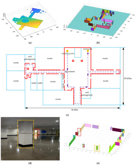
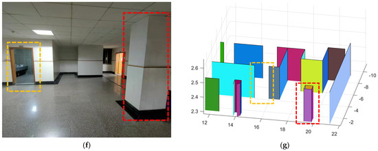
Figure 23.
The resulting presentation of scene 2: (a) point cloud data of scene 2; (b) the experimental results obtained by our algorithm; to better show the interior, we removed the ceiling; (c) we provide the two-dimensional plan of the floor and mark out the rooms, the toilets, the safe passage, and our movements; the gaps between the lines are the doors; (d,e) are the first part of the real scene and the comparison of experimental results; (f,g) are the second part of the real scene and the comparison of experimental results.
Comparing the results with the real scene, we can see that all the walls are well restored. At the time of measurement, we did not enter any rooms. Some of the doors were open and others were closed, which is why some of the doors were empty in our results. At the same time, due to the attention to detail in our method, uneven sampling and the error of the matching algorithm may result in faults in the same plane.
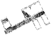
3.2.3. Experiment Scene 3
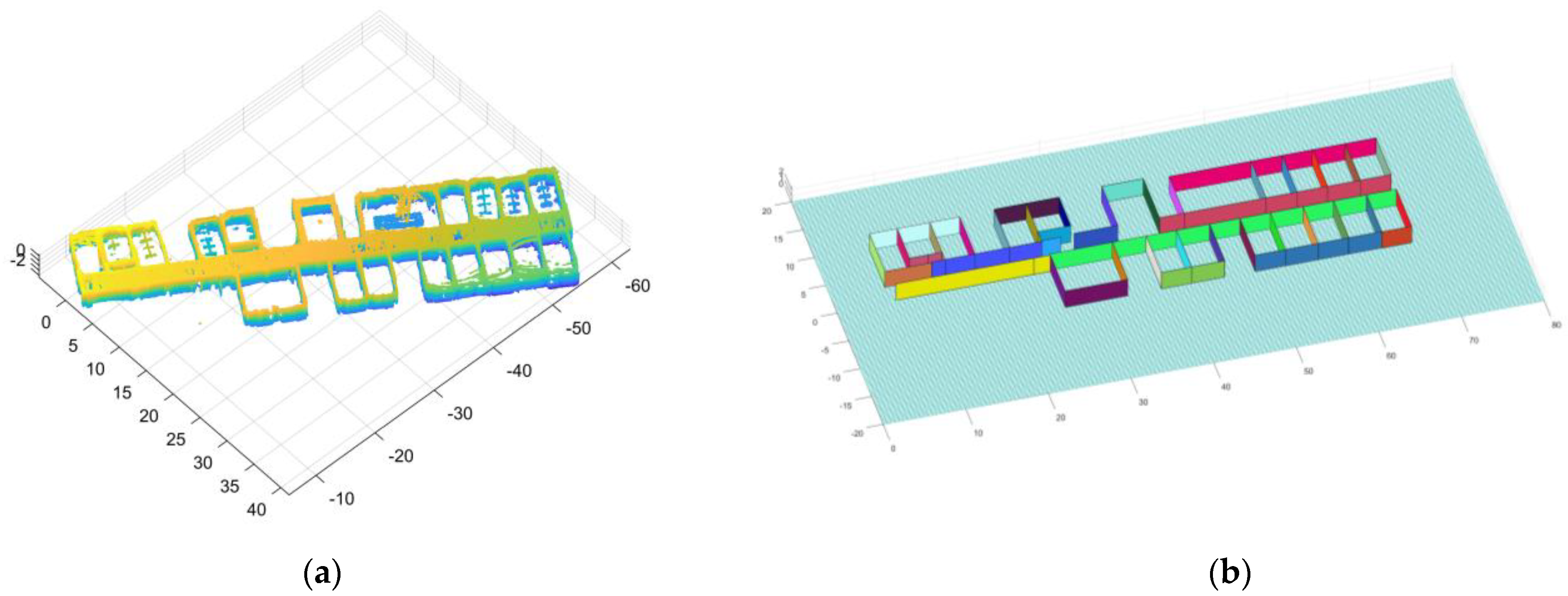
In scene 3, we chose an interior environment with multiple rooms. The raw data are shown in Figure 24a, and the result is shown in Figure 24b. We drew the two-dimensional plan of the data as shown in Figure 24c and a comparison of the result with the real world as shown in Figure 24d,e.

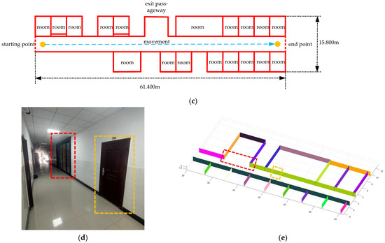
Figure 24.
The resulting presentation of scene 3: (a) point cloud data of scene 3; (b) the experimental results; (c) the two-dimensional plan of the data; we moved and scanned each room for a few seconds as we passed it; (d,e) we marked two locations in the simulation results that corresponded to the real world.
We entered most of the rooms during the measurement and all the doors were closed. Due to the complexity of the scene corresponding to the data, there was a major difference between the two frames when the device entered the room, which led to a major error in scan registration. Therefore, the error of our results is larger than that of the first two data points. However, all the rooms were restored well, so the result was satisfactory.
3.2.4. Relevant Parameters of the Experiment
We aim to obtain indoor structural information in a fast and efficient way, so we list running time, data volume, and distance parameters. In our approach, we employed a series of ways to reduce the amount of data. Therefore, on the premise of ensuring the authenticity and validity of parameters, and to demonstrate the efficiency of our method, we calculated the time of the following parts in Table 6: the time of fitting the ceiling and ground, the time of projection, filtering, and voxelization, and the time from image to three-dimensional reconstruction. To reflect the changes in the amount of data in the process, we counted the number of initial points, the number of wall points, the number of two-dimensional points after projection and voxelization, and the size of the image, as shown in Table 7. To verify the accuracy of the algorithm, we compare it with the actual data using the following aspects in Table 8 and Table 9: ceiling equation and ground equation after first calculation, the number of planes, the length , width , height of the building simulation data, the length , width , height of the building real data, the error between the actual value and the predicted value of the three aspects , , , and the mean precision . In Table 10, we list the characteristics of different reconstruction methods in recent years. The function and purpose of each method are not completely the same. To reflect the innovation of our method and solve the problem, we evaluate it while considering the following aspects: (1) sources of data; the effect of the algorithm can be affected by different data; (2) ground calculation; the ground is found as the base by our method without any conditions such as LiDAR attitude; (3) filtering; if no filtering is used, the algorithm has strong robustness; (4) data optimization; data optimization shows that the algorithm has high processing performance; (5) the manifestation of doors and windows; the details show the precision of the algorithm; (6) accuracy of the number of planes; if all planes are found, the accuracy of the algorithm is high.
Table 6.
The running time of several algorithms.
Table 7.
The data volume statistics of several steps algorithm.
Table 8.
Fitting the parameters of the ceiling and floor equations.
Table 9.
Parameter comparison between the actual scenario and the predicted scenario.
Table 10.
Comparison of the characteristics of several different methods. Aspect 1: sources of data; Aspect 2: ground calculation; Aspect 3: filtering; Aspect 4: data optimization; Aspect 5: the manifestation of doors and windows; Aspect 6: accuracy of the number of planes.
4. Discussion
First, we evaluated the experimental results of the three scenarios. In scenario 1, all vertical planes of the room are created and the basic structure is restored. Because of the curtain, the curved part is removed by our algorithm, which leads to gaps in the plane formed by the curtain. In our algorithm, we expand the coordinates of the data, and the uneven sampling areas and the walls with windows contain fewer points. These areas are removed by our method. Therefore, our method can better restore the details of the room by enlarging the coordinates, while the room is restored to a rectangle if normal processing is used. In scenario 2, due to the large area of the scene, we stretched the result vertically for better detail. We can see that all the open doors are identified as gaps between the planes, and by comparing the coordinates in the result, we can ensure that the plane precision is high; for example, the width of the door is about 1 m. The whole floor is well restored, although there are still a few errors in the plan. This is where our method will need to be optimized at a later stage. In scenario 3, we went into some rooms selectively, and the results show that the reconstruction is better. All the rooms are perfectly reproduced, though there are some errors due to scan registration.
Second, we analyze and discuss the parameters in five tables. In Table 6, although we optimized the filtering, we can see that most of the time is still spent on filtering and voxelization. However, in terms of the time and effect of restoring the image to a three-dimensional plane, the time of about 2 s shows that our slope-based algorithm is efficient and fast. Therefore, we will try other filtering approaches to improve the performance of the program in subsequent work. In Table 7, we can see a gradual decrease in the amount of data, such as in scene 3, the number of points is reduced to 187 × 52 from 1,568,974 × 3, which is why our approach is efficient. In Table 8, by comparing the parameters of the ceiling and ground planes, we note that they are parallel. The error of the room height calculated from these two planes is small (the maximum error does not exceed 0.015), so our method of finding the plane is accurate. We want to restore a model from the point cloud that is the same size as in the actual scene. In Table 9, by comparing the calculated length, width, and height with the actual value, the error between the predicted value and the actual value is, respectively, less than 0.044 m, 0.045 m, and 0.015 m. The mean error of 0.024 m proves that our algorithm is accurate within the error tolerance. In Table 10, we overcome the difficulty of LiDAR data processing and achieve similar results compared with some current methods. The data from LiDAR are easy to obtain but difficult to process, laser scanner data are difficult to obtain but high precision. We summarize the advantages and disadvantages of some algorithms. Then, we propose some methods to optimize and solve these problems in terms of prior knowledge, noise removal, data optimization, structure extraction, algorithm efficiency, and accuracy. Compared with existing methods, our method is superior to current algorithms in some respects.
Finally, there are still some shortcomings in our experiment. To make the initial data tidier, we will test other algorithms to replace the current algorithm for scan registration, such as LIO-SAM. Our method is currently only applicable to the reconstruction of interior vertical walls, and circles are recognized as polygons by the method. Therefore, we will modify the algorithm to accommodate more complex cases and make it more robust.
5. Conclusions
The method proposed in this paper can restore basic interior structure on an equal scale. In this method, the ceiling and the floor of the room are segmented and fitted, and the ground plane is used as the reference plane. Then, the wall is projected onto the reference plane. We filter, regularize, and transform the resulting two-dimensional data into an image. We extract the skeleton of the image and calculate the slope for each point. The slope that characterizes a line expands by growing until all points of the line are found. These lines are optimized and corrected by our method to produce more accurate lines. Finally, these lines are restored to three-dimensional vertical planes by applying height information. From the experimental results, the reconstruction effect and parameter analysis all show that our method is accurate (mean error of 0.024 m at an average measuring range of 40 m). In the whole algorithm, we pay attention to the improvement of computing speed and innovation of the algorithm. Therefore, we made a lot of data optimization and algorithm improvement, and we proposed a new framework to solve the problem of indoor reconstruction. However, there are some limitations and errors in this method. For example, parameters need to be adjusted to obtain the best results, and indoor sundries cannot be reconstructed. Therefore, we will focus on algorithm optimization and detail processing to make the algorithm more practical in the future.
Author Contributions
Conceptualization, J.Z.; methodology, J.Z. and D.C.; software, D.C.; validation, D.Z. and J.C.; formal analysis, J.Z. and D.C.; resources, D.T.; data curation, D.T.; writing—original draft preparation, D.C.; writing—review and editing, J.Z., D.C. and D.Z.; visualization, D.C.; supervision, J.Z. and J.C.; project administration, J.Z. All authors have read and agreed to the published version of the manuscript.
Funding
National Natural Science Foundation of China (62105372), Foundation of Key Laboratory of National Defense Science and Technology (6142401200301), Natural Science Foundation of Hunan Province (2021JJ40794).
Institutional Review Board Statement
Not applicable.
Informed Consent Statement
Not applicable.
Data Availability Statement
Not applicable.
Conflicts of Interest
The authors declare no conflict of interest.
References
- Geiger, A.; Lenz, P.; Stiller, C.; Urtasun, R. Vision meets robotics: The KITTI dataset. Int. J. Robot. Res. 2013, 32, 1231–1237. [Google Scholar] [CrossRef] [Green Version]
- Jo, K.; Kim, J.; Kim, D.; Jang, C.; Sunwoo, M. Development of Autonomous Car—Part II: A Case Study on the Implementation of an Autonomous Driving System Based on Distributed Architecture. IEEE Trans. Ind. Electron. 2015, 62, 5119–5132. [Google Scholar] [CrossRef]
- Yao, S.; Zhang, J.; Hu, Z.; Wang, Y.; Zhou, X. Autonomous-driving vehicle test technology based on virtual reality. J. Eng. 2018, 2018, 1768–1771. [Google Scholar] [CrossRef]
- Yaqoob, I.; Khan, L.U.; Kazmi, S.M.A.; Imran, M.; Guizani, N.; Hong, C.S. Autonomous Driving Cars in Smart Cities: Recent Advances, Requirements, and Challenges. IEEE Netw. 2020, 34, 174–181. [Google Scholar] [CrossRef]
- Urmson, C.; Anhalt, J.; Bagnell, D.; Baker, C.; Bittner, R.; Clark, M.N.; Dolan, J.; Duggins, D.; Galatali, T.; Geyer, C.; et al. Autonomous driving in urban environments: Boss and the Urban Challenge. J. Field Robot. 2008, 25, 425–466. [Google Scholar] [CrossRef] [Green Version]
- Gelbart, A.; Weber, C.; Bybee-Driscoll, S.; Freeman, J.; Fetzer, G.J.; Seales, T.; McCarley, K.A.; Wright, J. FLASH lidar data collections in terrestrial and ocean environments. In Proceedings of the SPIE 5086, Laser Radar Technology and Applications VIII, Orlando, FL, USA, 21 August 2003; pp. 27–38. [Google Scholar] [CrossRef]
- Kopp, F. Wake-vortex characteristics of military-type aircraft measured at Airport Oberpfaffenhofen using the DLR Laser Doppler Anemometer. Aerosp. Sci. Technol. 1999, 3, 191–199. [Google Scholar] [CrossRef]
- Zhou, L.F.; Yu, H.W.; Lan, Y. Deep Convolutional Neural Network-Based Robust Phase Gradient Estimation for Two-Dimensional Phase Unwrapping Using SAR Interferograms. IEEE Trans. Geosci. Remote Sens. 2020, 58, 4653–4665. [Google Scholar] [CrossRef]
- Zhou, L.F.; Yu, H.W.; Lan, Y.; Xing, M.D. Artificial Intelligence In Interferometric Synthetic Aperture Radar Phase Unwrapping: A Review. IEEE Geosci. Remote Sens. Mag. 2021, 9, 10–28. [Google Scholar] [CrossRef]
- Matayoshi, N.; Asaka, K.; Okuno, Y. Flight Test Evaluation of a Helicopter Airborne Lidar. J. Aircr. 2007, 44, 1712–1720. [Google Scholar] [CrossRef]
- Rabadan, G.J.; Schmitt, N.P.; Pistner, T.; Rehm, W. Airborne Lidar for Automatic Feedforward Control of Turbulent In-Flight Phenomena. J. Aircr. 2010, 47, 392–403. [Google Scholar] [CrossRef]
- Tachella, J.; Altmann, Y.; Mellado, N.; McCarthy, A.; Tobin, R.; Buller, G.S.; Tourneret, J.Y.; McLaughlin, S. Real-time 3D reconstruction from single-photon lidar data using plug-and-play point cloud denoisers. Nat. Commun. 2019, 10, 4984. [Google Scholar] [CrossRef] [Green Version]
- Yang, L.; Sheng, Y.; Wang, B. LiDAR data reduction assisted by optical image for 3D building reconstruction. Optik 2014, 125, 6282–6286. [Google Scholar] [CrossRef]
- Li, H.Y.; Yang, C.; Wang, Z.; Wu, G.L.; Li, W.H.; Liu, C. A Hierarchical Contour Method for Automatic 3d City Reconstruction From Lidar Data. In Proceedings of the 2012 IEEE International Geoscience and Remote Sensing Symposium, Munich, Germany, 22–27 July 2012; pp. 463–466. [Google Scholar] [CrossRef]
- Guiyun, Z.; Bin, W.; Ji, Z. Automatic Registration of Tree Point Clouds From Terrestrial LiDAR Scanning for Reconstructing the Ground Scene of Vegetated Surfaces. IEEE Geosci. Remote Sens. Lett. 2014, 11, 1654–1658. [Google Scholar] [CrossRef]
- Hu, H.; Fernandez-Steeger, T.M.; Dong, M.; Azzam, R. Numerical modeling of LiDAR-based geological model for landslide analysis. Autom. Constr. 2012, 24, 184–193. [Google Scholar] [CrossRef]
- Kim, C.; Habib, A. Object-Based Integration of Photogrammetric and LiDAR Data for Automated Generation of Complex Polyhedral Building Models. Sensors 2009, 9, 5679–5701. [Google Scholar] [CrossRef] [PubMed]
- Kwak, E.; Habib, A. Automatic representation and reconstruction of DBM from LiDAR data using Recursive Minimum Bounding Rectangle. ISPRS J. Photogramm. Remote Sens. 2014, 93, 171–191. [Google Scholar] [CrossRef]
- Liu, S.; Atia, M.M.; Karamat, T.B.; Noureldin, A. A LiDAR-Aided Indoor Navigation System for UGVs. J. Navig. 2014, 68, 253–273. [Google Scholar] [CrossRef] [Green Version]
- Liu, Y.; Fan, B.; Meng, G.; Lu, J.; Xiang, S.; Pan, C. DensePoint: Learning Densely Contextual Representation for Efficient Point Cloud Processing. In Proceedings of the 2019 IEEE/CVF International Conference on Computer Vision (ICCV), Seoul, Korea, 27 October–2 November 2019; pp. 5238–5247. [Google Scholar]
- Khatamian, A.; Arabnia, H.R. Survey on 3D Surface Reconstruction. J. Inf. Process. Syst. 2016, 12, 338–357. [Google Scholar] [CrossRef] [Green Version]
- Matiukas, V.; Paulinas, M.; Usinskas, A.; Adaskevicius, R.; Meskauskas, R.; Valincius, D. A survey of point cloud reconstruction methods. Electr. Control Technol. 2008, 3, 150–153. [Google Scholar]
- Valero, E.; Adan, A.; Cerrada, C. Automatic construction of 3D basic-semantic models of inhabited interiors using laser scanners and RFID sensors. Sensors 2012, 12, 5705–5724. [Google Scholar] [CrossRef] [Green Version]
- Shan, T.X.; Englot, B. LeGO-LOAM: Lightweight and Ground-Optimized Lidar Odometry and Mapping on Variable Terrain. In Proceedings of the 2018 IEEE/RSJ International Conference on Intelligent Robots and Systems (IROS), Madrid, Spain, 1–5 October 2018; pp. 4758–4765. [Google Scholar]
- Shan, T.; Englot, B.; Meyers, D.; Wang, W.; Ratti, C.; Rus, D. LIO-SAM: Tightly-coupled Lidar Inertial Odometry via Smoothing and Mapping. In Proceedings of the 2020 IEEE/RSJ International Conference on Intelligent Robots and Systems (IROS), Las Vegas, NV, USA, 24 October–24 January 2020; pp. 5135–5142. [Google Scholar]
- Ochmann, S.; Vock, R.; Wessel, R.; Klein, R. Automatic reconstruction of parametric building models from indoor point clouds. Comput. Graph. 2016, 54, 94–103. [Google Scholar] [CrossRef] [Green Version]
- Ochmann, S.; Vock, R.; Klein, R. Automatic reconstruction of fully volumetric 3D building models from oriented point clouds. ISPRS J. Photogramm. Remote Sens. 2019, 151, 251–262. [Google Scholar] [CrossRef] [Green Version]
- Schnabel, R.; Wahl, R.; Klein, R. Efficient RANSAC for point-cloud shape detection. Comput. Graph. Forum. 2007, 26, 214–226. [Google Scholar] [CrossRef]
- Saval-Calvo, M.; Azorin-Lopez, J.; Fuster-Guillo, A.; Garcia-Rodriguez, J. Three-dimensional planar model estimation using multi-constraint knowledge based on k-means and RANSAC. Appl. Soft Comput. 2015, 34, 572–586. [Google Scholar] [CrossRef] [Green Version]
- Ambrus, R.; Claici, S.; Wendt, A. Automatic Room Segmentation From Unstructured 3-D Data of Indoor Environments. IEEE Robot. Autom. Lett. 2017, 2, 749–756. [Google Scholar] [CrossRef]
- Sanchez, V.; Zakhor, A. Planar 3d Modeling of Building Interiors From Point Cloud Data. In Proceedings of the 2012 IEEE International Conference on Image Processing (ICIP 2012), Orlando, FL, USA, 30 September–3 October 2012; pp. 1777–1780. [Google Scholar]
- Wang, C.; Cho, Y.K.; Kim, C. Automatic BIM component extraction from point clouds of existing buildings for sustainability applications. Autom. Constr. 2015, 56, 1–13. [Google Scholar] [CrossRef]
- Mura, C.; Mattausch, O.; Jaspe Villanueva, A.; Gobbetti, E.; Pajarola, R. Automatic room detection and reconstruction in cluttered indoor environments with complex room layouts. Comput. Graph. 2014, 44, 20–32. [Google Scholar] [CrossRef] [Green Version]
- Oesau, S.; Lafarge, F.; Alliez, P. Indoor scene reconstruction using feature sensitive primitive extraction and graph-cut. ISPRS J. Photogramm. Remote Sens. 2014, 90, 68–82. [Google Scholar] [CrossRef] [Green Version]
- Palomba, C.; Astone, P.; Frasca, S. Adaptive Hough transform for the search of periodic sources. Class. Quant. Grav. 2005, 22, S1255–S1264. [Google Scholar] [CrossRef] [Green Version]
- Wu, H.; Yue, H.; Xu, Z.; Yang, H.; Liu, C.; Chen, L. Automatic structural mapping and semantic optimization from indoor point clouds. Autom. Constr. 2021, 124, 103460. [Google Scholar] [CrossRef]
- Wang, C.; Cho, Y. Automated 3D building envelope recognition from point clouds for energy analysis. In Proceedings of the Construction Research Congress 2012: Construction Challenges in a Flat World, West Lafayette, IN, USA, 21–23 May 2012; pp. 1155–1164. [Google Scholar]
- Xiong, X.; Adan, A.; Akinci, B.; Huber, D. Automatic creation of semantically rich 3D building models from laser scanner data. Autom. Constr. 2013, 31, 325–337. [Google Scholar] [CrossRef] [Green Version]
- Tang, S.; Zhang, Y.; Li, Y.; Yuan, Z.; Wang, Y.; Zhang, X.; Li, X.; Zhang, Y.; Guo, R.; Wang, W. Fast and Automatic Reconstruction of Semantically Rich 3D Indoor Maps from Low-quality RGB-D Sequences. Sensors 2019, 19, 533. [Google Scholar] [CrossRef] [Green Version]
- Tang, S.; Zhu, Q.; Chen, W.; Darwish, W.; Wu, B.; Hu, H.; Chen, M. Enhanced RGB-D Mapping Method for Detailed 3D Indoor and Outdoor Modeling. Sensors 2016, 16, 1589. [Google Scholar] [CrossRef] [PubMed] [Green Version]
- Stojanovic, V.; Trapp, M.; Richter, R.; Döllner, J. A service-oriented approach for classifying 3D points clouds by example of office furniture classification. In Proceedings of the 23rd International ACM Conference on 3D Web Technology, Poznań, Poland, 20–22 June 2018; pp. 1–9. [Google Scholar]
- Jung, J.; Hong, S.; Yoon, S.; Kim, J.; Heo, J. Automated 3D Wireframe Modeling of Indoor Structures from Point Clouds Using Constrained Least-Squares Adjustment for As-Built BIM. J. Comput. Civ. Eng. 2016, 30, 04015074. [Google Scholar] [CrossRef]
- Jung, J.; Stachniss, C.; Kim, C. Automatic Room Segmentation of 3D Laser Data Using Morphological Processing. ISPRS Int. J. Geo-Inf. 2017, 6, 206. [Google Scholar] [CrossRef] [Green Version]
- Saeed, K.; Tabędzki, M.; Rybnik, M.; Adamski, M. K3M: A universal algorithm for image skeletonization and a review of thinning techniques. Int. J. Appl. Math. Comput. Sci. 2010, 20, 317–335. [Google Scholar] [CrossRef]
- Zhang, T.Y.; Suen, C.Y. A fast parallel algorithm for thinning digital patterns. Commun. ACM 1984, 27, 236–239. [Google Scholar] [CrossRef]
- Harris, C.; Stephens, M. A combined corner and edge detector. In Proceedings of the Alvey Vision Conference, Manchester, UK, 31 August–2 September 1988; pp. 10–5244. [Google Scholar]
- Smith, S.M.; Brady, J.M. SUSAN—A new approach to low level image processing. Int. J. Comput. Vis. 1997, 23, 45–78. [Google Scholar] [CrossRef]
- Chen, S.; Meng, H.; Zhang, C.; Liu, C. A KD curvature based corner detector. Neurocomputing 2016, 173, 434–441. [Google Scholar] [CrossRef]
- Renzhong, L.; Man, Y.; Yuan, R.; Huanhuan, Z.; Junfeng, J.; Pengfei, L. Point cloud denoising and simplification algorithm based on method library. Laser Optoelectron. Prog. 2018, 55, 1–4. [Google Scholar] [CrossRef]


Publisher’s Note: MDPI stays neutral with regard to jurisdictional claims in published maps and institutional affiliations. |
© 2021 by the authors. Licensee MDPI, Basel, Switzerland. This article is an open access article distributed under the terms and conditions of the Creative Commons Attribution (CC BY) license (https://creativecommons.org/licenses/by/4.0/).