Object-Based Wetland Vegetation Classification Using Multi-Feature Selection of Unoccupied Aerial Vehicle RGB Imagery

Abstract

Wetland vegetation is an important component of wetland ecosystems and plays a crucial role in the ecological functions of wetland environments. Accurate distribution mapping and dynamic change monitoring of vegetation are essential for wetland conservation and restoration. The development of unoccupied aerial vehicles (UAVs) provides an efficient and economic platform for wetland vegetation classification. In this study, we evaluated the feasibility of RGB imagery obtained from the DJI Mavic Pro for wetland vegetation classification at the species level, with a specific application to Honghu, which is listed as a wetland of international importance. A total of ten object-based image analysis (OBIA) scenarios were designed to assess the contribution of five machine learning algorithms to the classification accuracy, including Bayes, K-nearest neighbor (KNN), support vector machine (SVM), decision tree (DT), and random forest (RF), multi-feature combinations and feature selection implemented by the recursive feature elimination algorithm (RFE). The overall accuracy and kappa coefficient were compared to determine the optimal classification method. The main results are as follows: (1) RF showed the best performance among the five machine learning algorithms, with an overall accuracy of 89.76% and kappa coefficient of 0.88 when using 53 features (including spectral features (RGB bands), height information, vegetation indices, texture features, and geometric features) for wetland vegetation classification. (2) The RF model constructed by only spectral features showed poor classification results, with an overall accuracy of 73.66% and kappa coefficient of 0.70. By adding height information, VIs, texture features, and geometric features to construct the RF model layer by layer, the overall accuracy was improved by 8.78%, 3.41%, 2.93%, and 0.98%, respectively, demonstrating the importance of multi-feature combinations. (3) The contribution of different types of features to the RF model was not equal, and the height information was the most important for wetland vegetation classification, followed by the vegetation indices. (4) The RFE algorithm effectively reduced the number of original features from 53 to 36, generating an optimal feature subset for wetland vegetation classification. The RF based on the feature selection result of RFE (RF-RFE) had the best performance in ten scenarios, and provided an overall accuracy of 90.73%, which was 0.97% higher than the RF without feature selection. The results illustrate that the combination of UAV-based RGB imagery and the OBIA approach provides a straightforward, yet powerful, approach for high-precision wetland vegetation classification at the species level, in spite of limited spectral information. Compared with satellite data or UAVs equipped with other types of sensors, UAVs with RGB cameras are more cost efficient and convenient for wetland vegetation monitoring and mapping.

1. Introduction

A wetland is a transitional zone between terrestrial and aquatic ecosystems, with multi-functions ranging from purifying the environment to regulating flood water, improving water quality and protecting biodiversity, among others [1,2]. Wetland vegetation, an important component of wetland ecosystems, plays a crucial role in the ecological functions of wetland environments. The dynamic change in wetland vegetation is closely related to the evolution of the environmental quality of the wetland [3]. Therefore, there is an emerging demand for the accurate monitoring and mapping of wetland vegetation distribution, which can provide a scientific basis for wetland protection and restoration [4].

Satellite remote sensing is an indispensable means for wetland assessment, providing abundant spatial information over large areas and compensating for traditional field surveys, which are expensive, time consuming, and scale-limited [5,6,7,8,9,10,11]. Previous studies have successfully performed dynamic monitoring of wetland vegetation at different scales, from the landscape [12] to community level [13], by using radar, multispectral and hyperspectral imagery. However, it is difficult to realize wetland vegetation classification at the species level with freely available medium–low-resolution satellite data, due to the high spatial and temporal variability of wetland vegetation [14,15]. Lane et al. [8] successfully employed Worldview-2 imagery with high spatial resolution (0.5 m) to identify wetland vegetation. However, in general, high-resolution satellite images are too expensive for many scientific studies. In addition to the resolution and price, weather conditions, a long returning period and a fixed orbit also limit the application of satellite remote sensing [5,16].

In recent years, unoccupied aerial vehicles (UAVs) have been increasingly used in environmental monitoring and management. As a new, low-altitude remote sensing technology, UAV remote sensing has the advantages of high flexibility, cost efficiency, and high spatial resolution, ranging from the submeter to centimeter level [15,17,18,19,20]. UAVs serve as platforms to carry different sensors, such as LiDAR, multispectral, hyperspectral, and RGB cameras [21], to acquire image data, especially in areas with poor accessibility. In particular, small consumer-level UAVs equipped with RGB cameras are more flexible and more affordable than UAVs with other sensors, and RGB images are straightforward to process and interpret [21,22,23,24]. Studies of forest monitoring, precision agriculture, and marine environment monitoring have been performed with UAV-based RGB imagery [21,23,24]. A review of the application of UAVs in wetlands [25] indicates that RGB sensors are the most commonly used sensors. UAV-based RGB imagery has also developed as an indispensable and promising means to conduct wetland vegetation monitoring and mapping [6,15,26,27,28].

However, the increased spatial resolution of UAV images also negatively impacts the classification results due to the large variations in spectral information within the same class, which is prone to the “salt-and-pepper” phenomenon when using the traditional pixel-based classification approach [29,30]. Object-based image analysis (OBIA) is a new classification method emerging as an alternative to traditional classification approaches to process high-resolution images [31,32]. Previous studies have verified that OBIA is a powerful approach for extracting multi-features, which benefits vegetation monitoring and mapping from high-resolution images [33,34,35]. OBIA first segments the images into homogeneous pixel aggregations using a segmentation algorithm, and then fully mines the semantic features of the images, such as the spectrum, texture, shape, topology, and context at the object level [36], which are set as the input to the machine learning algorithms, to differentiate objects [37]. Several common machine learning algorithms have been implemented in object-based wetland vegetation mapping, such as fully convolutional networks (FCN), deep convolutional neural networks (DCNN) [37], random forest (RF) [38], and support vector machine (SVM) [32]. According to previous studies, RF and SVM are the most widely used models in classification research [39,40,41]. In addition, Bayes, K-nearest neighbor (KNN), and decision tree (DT) are also widely used in OBIA [42], such as the mapping of asbestos cement roofs being implemented by Bayes and KNN [43], and land cover classification being realized by DT [44]. However, massive features acquired through OBIA may reduce the classification performance of machine learning algorithms when there is a large number of features over a finite subset [45]. Feature selection is a crucial step to optimize classification accuracy by eliminating irrelevant or redundant variables [46]. Cao et al. [47] used OBIA to classify mangrove species based on UAV hyperspectral images, and the results showed that feature selection effectively improved the classification accuracy of the SVM model from 88.66% to 89.55%. Zuo et al. [48] also pointed out that feature selection improved the accuracy of the RF model in object-based marsh vegetation classification, with an overall accuracy of 87.12% and kappa coefficient of 0.850, and the overall accuracy of the RF model without feature selection was less than 80%. Abeysinghe et al. [33] emphasized the influence of feature selection on machine learning classifiers when mapping Phragmites australis based on UAV multispectral images.

Taking the cost of multispectral and hyperspectral sensors into consideration, UAVs with RGB cameras are preferable for vegetation monitoring and mapping [25]. Digital orthophoto maps (DOM), digital surface models (DSM), and point clouds derived from RGB imagery provide multi-features for wetland vegetation classification. Therefore, machine learning algorithms based on feature selection enable UAV-based RGB imagery to achieve high-precision wetland vegetation classification, despite the limited spectral information. Bhatnagar et al. [26] used RF and the convolutional neural network (CNN) for raised bog vegetation mapping based on UAV RGB imagery, and the results showed that the classification accuracy of the CNN, based on multi-features, was over 90%. Both the studies of Boon et al. [49] and Corti Meneses et al. [27] highlighted that the combination of point clouds, DSM, and DOM can provide a more accurate description of wetland vegetation. Although good classification accuracy was achieved, few scholars have comprehensively evaluated the importance of multi-features and the performance of different machine learning algorithms based on UAV RGB imagery for wetland vegetation classification.

We aim to identify a cost-efficient and accurate method for wetland vegetation classification by evaluating the contribution of multi-features and machine learning algorithms, and exploring the applicability of UAV-based RGB imagery in wetland vegetation classification at the species level. We chose a vegetation-rich area in the south of the Honghu wetland as the research area, and used DOM and DSM, derived from the UAV-based RGB imagery, as the data source. The spectral information (RGB), vegetation indices (VIs), texture features, and geometric features were fully extracted from DOM, and the relative height information of vegetation was obtained from DSM. Specifically, we designed ten object-based classification scenarios to achieve the following objectives: (1) comprehensively compare the classification performance of Bayes, KNN, SVM, DT, and RF, to identify the best machine learning algorithm; (2) assess the contribution of different features to the best machine learning algorithm; (3) evaluate the effectiveness of feature selection to improve the classification accuracy of the best machine learning algorithm. This paper looks forward to realizing object-based classification of wetland vegetation in an economical, efficient and high-precision way, by using UAV-based RGB imagery.

2. Material and Methods

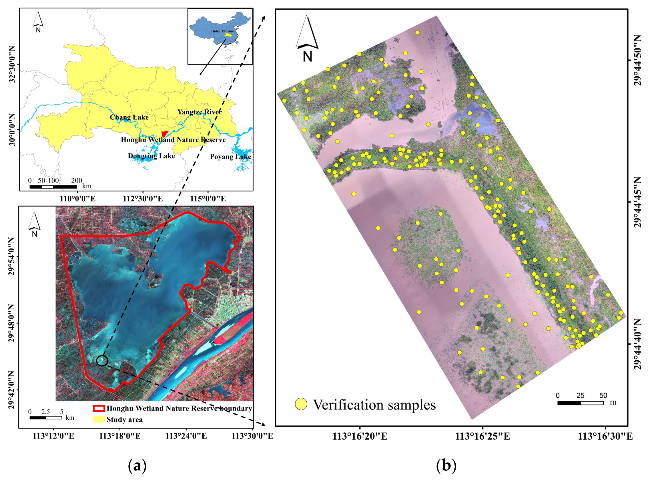
2.1. Study Area

Honghu wetland (29°41′–29°58′N, 113°12′–113°28′E; Figure 1) is located in Southern Hubei Province and has a surface area of approximately 414 km². As the seventh largest freshwater lake in China, Honghu was listed as an international important wetland under the Ramsar Convention in 2008 [50]. The study area belongs to a subtropical humid monsoon climate, with mean air temperatures ranging from +3.8 °C in January to +28.9 °C in July and annual mean precipitation ranging from 1000 mm to 1300 mm. Honghu Lake is a typical shallow lake formed by sediment silt with flat terrain, showing a zonal distribution of plants. More than 100 species of vegetation have been found in Honghu wetland during the field survey after 2010 [51], such as Humulus scandens, Alternanthera philoxeroides, Setaria viridis, Acalypha australis, Polygonum lapathifolium, Polygonum perfoliatum, Nelumbo nucifera, Zizania latifolia, Phragmites communis, Eichhornia crassipes, Potamogeton crispus, etc. The high plant biodiversity in Honghu wetland makes it a suitable and representative place for wetland vegetation classification.

2.2. Data Acquisition and Pre-Processing

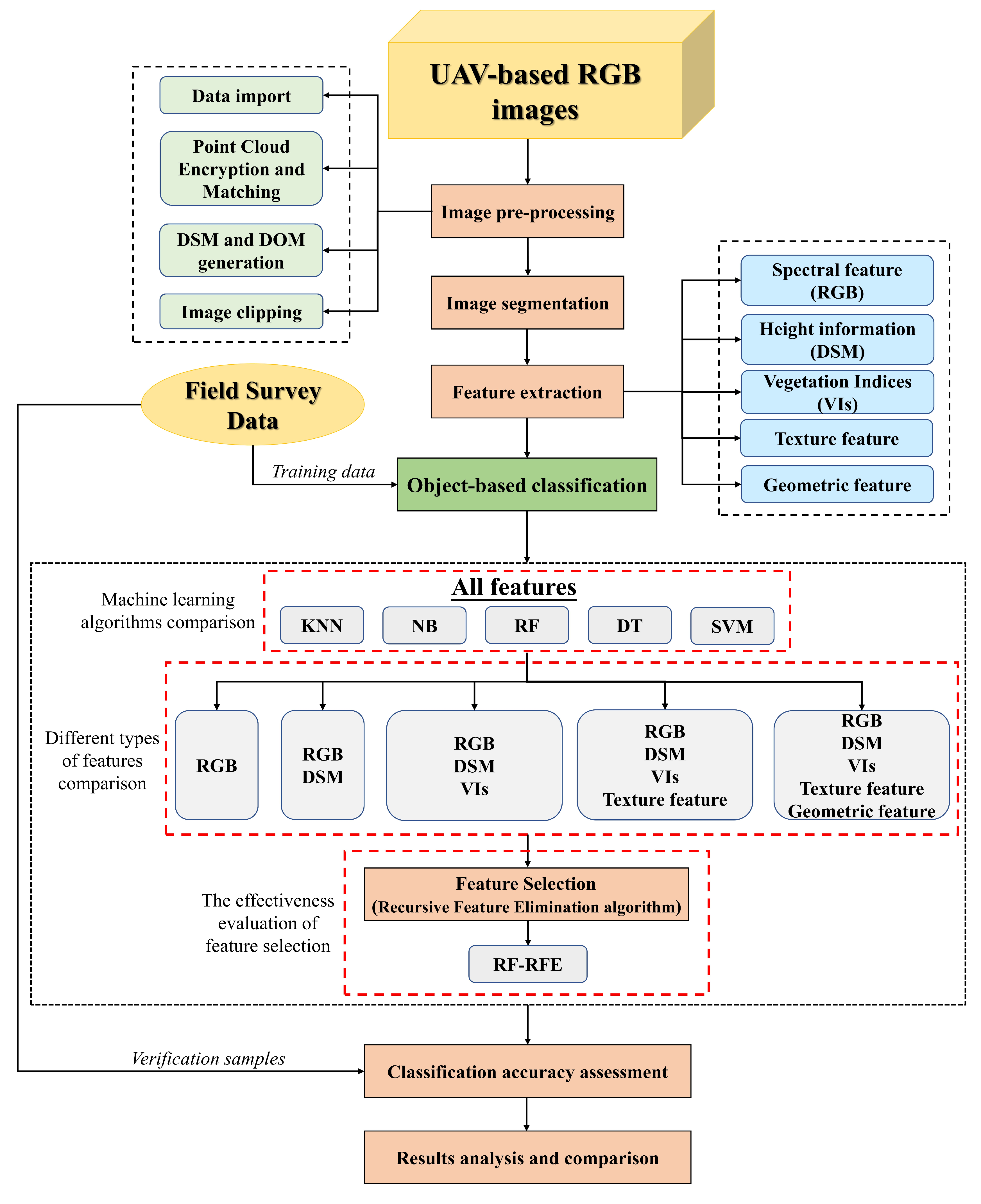
We conducted a wetland vegetation field survey on 12 May 2021, and collected UAV-based RGB imagery from 11:00 a.m. to 12:00 p.m. using a DJI Mavic Pro with an L1D-20c camera. The UAV task was deployed at an altitude of 50 m, forward overlap of 80% and lateral overlap of 70% with clear and windless weather conditions. A total of 314 RGB images were obtained with a ground resolution of 1.16 cm. Pix4Dmapper was used to pre-process RGB images in the following three steps: (1) import 314 images into the software; (2) point cloud encryption and matching; (3) generation of DOM and DSM. We clipped image data and selected areas containing abundant aquatic vegetation as the study area according to the research requirement.

A ground verification sample collection was carried out simultaneously, and a total of 205 samples were obtained to assess the accuracy of ten classification scenarios. A handheld GPS was used to record the exact location of the samples in the accessible area. A DJI Mini2 was deployed to take photos in hovering mode at a height of 5–10 m to acquire verification samples from inaccessible areas. The vegetation type of these photographic verification samples was identified with the assistance of aquatic vegetation experts. Based on the official website, the horizontal positioning accuracy of DJI Mini2 is within ±0.1 m when the weather is cloudless and windless. Therefore, the location information of the verification samples was obtained from the photos, and it met the research requirements for wetland vegetation classification. According to the field survey, the following eight aquatic vegetation classes and two non-vegetation classes were identified in the study area: Zizania latifolia, Phragmites australis, Nelumbo nucifera, Alternanthera philoxeroides, Sambucus chinensis, Polygonum perfoliatum, Triarrhena lutarioriparia, water, tree shrubs (including Melia Azedarach, Pterocarya stenoptera, Broussonetia Papyrifera, Populus Euramevicana, and Sapium Sebiferum) and other (non-vegetation and non-water bodies).

2.3. Study Workflow

In this study, UAV-based RGB imagery was used to classify wetland vegetation with OBIA and feature selection. The methodology included the following six main phases: (1) optimal segmentation parameter determination and image segmentation; (2) 53 features derived from DOM and DSM; (3) comparison of machine learning algorithms based on 53 features; (4) evaluation of the contribution of different types of features; (5) effectiveness evaluation of feature selection; (6) accuracy assessment of ten object-based classification scenarios. Figure 2 shows the workflow of this study.

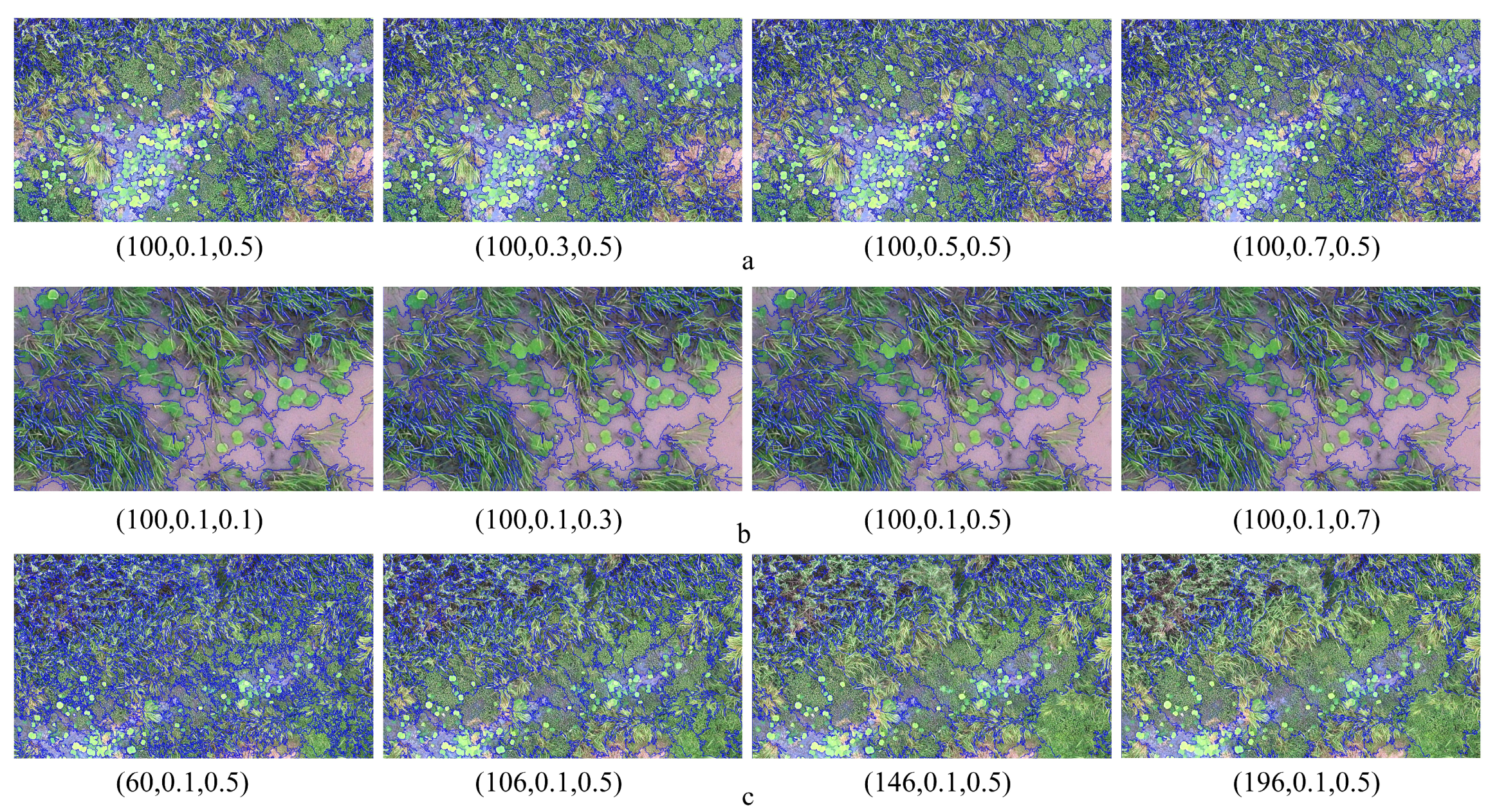
2.3.1. Image Segmentation

In our study, Trimble eCognition Developer 9.0, an object-based image analysis software, was used to implement efficient image segmentation through the multi-resolution segmentation algorithm [52]. The image segmentation process adopts the bottom-up region merging technique to merge adjacent pixels together based on the principle of minimum heterogeneity [53] to generate objects with similar or identical features. The multi-resolution segmentation algorithm contains the following four important parameters: layer weights, scale, shape index and compactness [54]. The setting of segmentation parameters affects the classification accuracy. The determination of segmentation parameters is generally performed by identifying the optimal parameter combination screened by repeated experiments and manual interpretation. In order to reduce the influence of subjective factors, we applied the estimation of scale parameter 2 (ESP2), a fast optimal segmentation scale selection tool. ESP2 generates the curves of local variance (LV) and rate of change (ROC) as a function of scale parameters, and the peak of the ROC curve represents the possible optimal segmentation scale [29].

2.3.2. Features Derived from DOM and DSM

Wetland vegetation distribution is greatly affected by factors such as water, soil and weather. It is challenging to distinguish wetland vegetation with homogenous spectral information from only optical information. Up to date, many scholars have explored the integration of multi-types of features to enhance the separability of vegetation [55,56,57]. In addition to spectral features (RGB), this paper also extracted height information, vegetation indices, texture and geometric features of the image objects generated by image segmentation for a total of 53 features for the next step of wetland vegetation classification and interpretation. The specific features are listed in

Table 1. Description of object features used in classification.

Feature Type	Feature Names	Feature Description	Feature Number
Spectral feature	Mean R, mean G, mean B, standard deviation R, standard deviation G, standard deviation B	R, G and B represent the DN value of red, green, and blue bands, respectively. Mean value and standard deviation for each object in the red, blue and green bands, calculated from the DN value of the object’s pixel.	7
	Brightness	Brightness is calculated from the combination of the DN value of the object’s pixel
Height information	Mean DSM, standard deviation DSM	Mean value and standard deviation for each object in DSM	2
Vegetation indices	Shown in Table 2		14
Texture feature	GLCM_Mean r, GLCM_Mean g, GLCM_Mean b, GLCM_ StdDev r, GLCM_ StdDev g, GLCM_ StdDev b, GLCM_ Ent r, GLCM_ Ent g, GLCM_ Ent b, GLCM_ASM r, GLCM_ASM g, GLCM_ASM b, GLCM_ Cor r, GLCM_ Cor g, GLCM_ Cor b, GLCM_ Dis r, GLCM_ Dis g, GLCM_ Dis b, GLCM_Con r, GLCM_Con g, GLCM_Con b, GLCM_Hom r, GLCM_Hom g, GLCM_Hom b	Standard deviation (StdDev), entropy (Ent), angular second moment (ASM), correlation (Cor), dissimilarity (Dis), contrast (Con), homogeneity (Hom), r: red band, g: green band, b: blue band Texture features are derived from red, green and blue bands by using gray-level co-occurrence matrix (GLCM).	24
Geometric feature	Area, compactness, roundness, shape index, density, asymmetry	Geometric features are calculated from the geometry information of the object.	6

.

(1)

Spectral features are the basic features of wetland vegetation identification. Mean value and standard deviation of the red, green, blue bands and brightness were extracted.

(2)

DSM was used to represent the relative height of wetland vegetation. Height information can increase the separability between vegetation types, especially in areas with dense vegetation [58]. Therefore, the mean value and standard deviation of DSM were also used for wetland vegetation classification.

(3)

Vegetation indices, serving as a supplement of vegetation spectral information, were constructed using the available red, green and blue spectral bands [59]. They effectively distinguish vegetation from the surrounding terrain background and greatly improve the application potential of UAV-based RGB imagery. A total of 14 frequently used vegetation indices were calculated (Table 2).

(4)

Texture features have been frequently applied for terrain classification [57] and successfully improved the accuracy of image classification and information extraction. The gray-level co-occurrence matrix (GLCM) was used to extract 24 texture features, including mean, standard deviation (StdDev), entropy (Ent), angular second moment (ASM), correlation (Cor), dissimilarity (Dis), contrast (Con) and homogeneity (Hom) of red, green and blue bands [60].

(5)

Geometric features have been shown to have a positive effect on vegetation classification [38,61], and the following six frequent geometric features were utilized in this study: area, compactness, roundness, shape index, density and asymmetry.

Table 2. Vegetation indices derived from RGB imagery (R, G and B represent the DN value of red, green, and blue bands, respectively).

Vegetation Indices	Full Name	Formulation	Reference
ExG	Excess green index	$2G-R-B$	[62]
ExGR	Excess green minus excess red index	$ExG-1.4R-G$	[35]
VEG	Vegetation index	$G/R^{0.67}{B}^{0.33}$	[35]
CIVE	Color index of vegetation	$0.44R-0.88G+0.39B+18.79$	[63]
COM	Combination index	$0.25ExG+0.3ExGR+0.33CIVE+0.12VEG$	[64]
COM2	Combination index 2	$0.36ExG+0.47CIVE+0.17VEG$	[63]
NGRDI	Normalized green–red difference index	$\left(G-R\right)/\left(G+R\right)$	[35]
NGBDI	Normalized green–blue difference index	$\left(G-B\right)/\left(G+B\right)$	[65]
VDVI	Visible-band difference vegetation index	$\left(2G-R-B\right)/\left(2G+R+B\right)$	[65]
RGRI	Red–green ratio index	$R/G$	[66]
BGRI	Blue–green ratio index	$B/G$	[67]
WI	Woebbecke index	$\left(G-B\right)/\left(R-G\right)$	[62]
RGBRI	Red–green–blue ratio index	$\left(R+B\right)/2G$	[68]
RGBVI	Red–green–blue vegetation	$(G^2-\left(R\ast B\right))/\left(G^2+\left(R\ast B\right)\right)$	[22]

Table 2. Vegetation indices derived from RGB imagery (R, G and B represent the DN value of red, green, and blue bands, respectively).

Vegetation Indices	Full Name	Formulation	Reference
ExG	Excess green index	$2G-R-B$	[62]
ExGR	Excess green minus excess red index	$ExG-1.4R-G$	[35]
VEG	Vegetation index	$G/R^{0.67}{B}^{0.33}$	[35]
CIVE	Color index of vegetation	$0.44R-0.88G+0.39B+18.79$	[63]
COM	Combination index	$0.25ExG+0.3ExGR+0.33CIVE+0.12VEG$	[64]
COM2	Combination index 2	$0.36ExG+0.47CIVE+0.17VEG$	[63]
NGRDI	Normalized green–red difference index	$\left(G-R\right)/\left(G+R\right)$	[35]
NGBDI	Normalized green–blue difference index	$\left(G-B\right)/\left(G+B\right)$	[65]
VDVI	Visible-band difference vegetation index	$\left(2G-R-B\right)/\left(2G+R+B\right)$	[65]
RGRI	Red–green ratio index	$R/G$	[66]
BGRI	Blue–green ratio index	$B/G$	[67]
WI	Woebbecke index	$\left(G-B\right)/\left(R-G\right)$	[62]
RGBRI	Red–green–blue ratio index	$\left(R+B\right)/2G$	[68]
RGBVI	Red–green–blue vegetation	$(G^2-\left(R\ast B\right))/\left(G^2+\left(R\ast B\right)\right)$	[22]

2.3.3. Machine Learning Algorithm Comparison

Previous studies have determined that different machine learning algorithms may show different classification performances [44,69,70]. Comparing machine learning algorithms often helps increase classification accuracy. In this study, five commonly used classifiers were applied to conduct object-based supervised classification in eCognition 9.0, for Bayes, KNN, DT, SVM and RF, respectively. In order to compare the performance of these classifiers in the application of wetland vegetation classification, all the 53 features were applied in the classifier training procedure, and the best classifier was selected for the follow-up research. The classifiers are introduced below.

● Bayes

Bayes is a simple probabilistic classification model based on the Bayesian theorem and assumes that features are unrelated to each other [43]. This algorithm uses training samples to estimate the mean vectors and covariance matrices for each class and then applies them for classification [44]. Bayes does not require many parameters, but may be subjective.

● K-nearest neighbor (KNN)

KNN is a commonly used nonlinear classifier and assumes similarities of neighboring objects. This algorithm seeks the K nearest neighbors in the feature space for the unclassified objects and identifies the unclassified objects through the features of its K nearest neighbors [43,44]. The parameter K is essential for the performance of the KNN classifier.

● Decision tree (DT)

DT is a typical non-parametric rule-based classifier and has great capability to handle data sets with large numbers of attributes. The algorithm is constructed from the training sample subset [71] and is composed of a root node with all the training samples, a set of internal nodes with splits, and a set of leaf nodes [72,73]. The class label of the unclassified objects is determined according to the leaf node to which the object belongs.

● Support vector machine (SVM)

SVM is a non-parametric algorithm based on the statistical learning theory that was first proposed by Vapnik and Cortes in 1995 [74]. It attempts to define the optimal linear separating hyperplane from the training samples based on the maximum gap and then identifies any two classes [70]. Polynomial and radial basis function kernels are often used to project non-linear classes into separable linear ones in a higher dimension [44]. SVM does not rely on the distribution of the data and is robust to train small training sample sets [42,75].

● Random forest (RF)

RF, first proposed by Breiman in 2001, is a novel machine learning method based on the statistical learning theory and composed of multiple decision trees [76]. Unlike traditional classification models with poor generalization ability, RF can significantly improve the accuracy of classification results, reduce the influence of outliers and avoid over-fitting [39]. The realization steps of RF are briefly summarized as follows: (1) use the bootstrap resampling method to select k training sample sets randomly with replacement; (2) build k decision trees for k sample sets; (3) select m features randomly from the original features and set m as per tree splitting node; (4) form the random forest with k constructed decision trees and use the random forest to predict the classification result. The RF model shows stable robustness in processing complex data and has been shown to have excellent predictive capability in ecology [77].

2.3.4. Contribution of Different Types of Features Evaluation

Multi-features derived from UAV-based RGB imagery are of great significance for wetland vegetation classification. Scholars are concerned about the contribution of different types of features to the performance of the classifier. Therefore, many studies gradually add different types of features into the same classifier layer by layer, analyzing the contribution of the features through the overall classification accuracy [38,48,78,79]. From the results of Section 3.2, RF provided higher accuracy than the other four machine learning algorithms. Therefore, spectral features, height information, VIs, texture features and geometric features are added layer by layer to construct the RF classifier to evaluate the contribution of different types of features.

2.3.5. Effectiveness Evaluation of Feature Selection

Feature selection plays a critical role in object-based classification processes [45]. Studies have shown that features that were generally chosen by experience have high subjectivity and unequal contributions to classification accuracy. Furthermore, redundant features will bring negative effects to the performance and stability of a classification model [56]. Therefore, it is necessary to optimize and reduce the number of features by eliminating those that are not relevant and achieve, simultaneously, the highest intra-cluster similarity and the lowest inter-cluster similarity [53]. There are three popular feature selection strategies, which are as follows: filter, wrapper and embedded methods. Filter methods rely on variable ranking techniques to select the feature subset with no irrelevance to the modeling algorithm, but generate a large scale of feature subsets [80]. Wrapper methods use the performance of the learning algorithm as the feature selection criterion. It has been confirmed that wrapper methods can generate more appropriate feature subsets than filter methods, but are more time consuming [81]. Feature selection procedures and learning algorithms are achieved synchronously in embedded methods with higher treatment efficiency, but often cause over-fitting and poor robustness [80,82].

Recursive feature elimination (RFE) is a typical wrapper method based on a greedy algorithm, first proposed by Guyon et al. [83] in 2002. The essence of RFE is removing one of the least relevant features through cyclic iteration until all features are traversed, and outputting the feature ranking list [41]. In this study, the RFE algorithm was implemented using the “caret” package within statistical software R. A 10-fold cross-validation was applied to evaluate the optimal feature subset [84] in the RFE algorithm. According to the feature selection result, the last RF classifier was constructed by the optimal feature subset (RF-RFE).

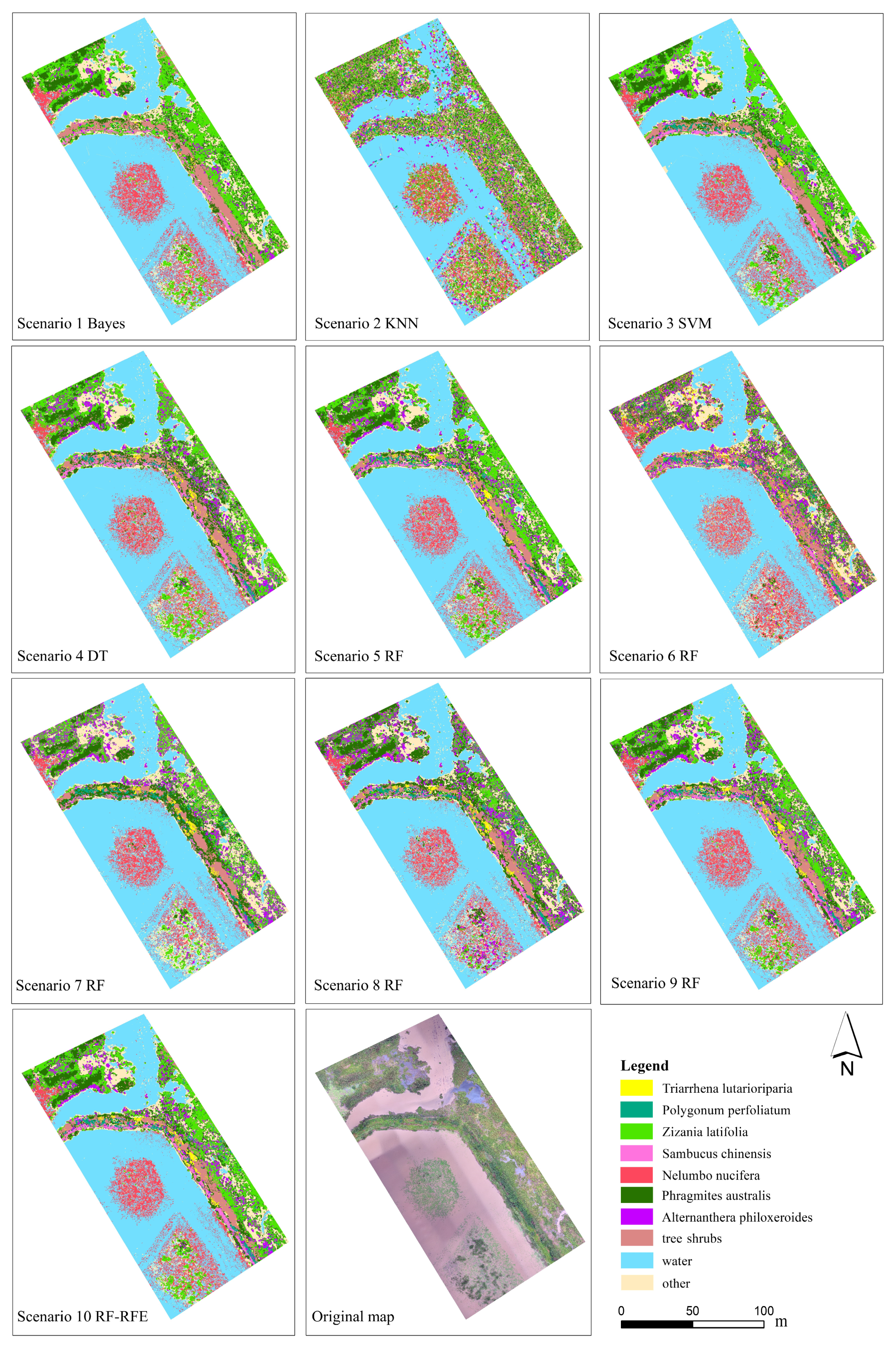
2.3.6. Ten Object-Based Classification Scenarios Design and Accuracy Assessment

In order to explore the performance of different machine learning algorithms, the contribution of different types of features and the effectiveness of feature selection, ten scenarios were designed for object-based wetland vegetation classification (

Table 3. Ten object-based classification scenarios design.

Scenario	Classification Model	Classification Features	Feature Number
1	Bayes	RGB+DSM+VIs+Texture+Geometry	53
2	KNN	RGB+DSM+VIs+Texture+Geometry	53
3	SVM	RGB+DSM+VIs+Texture+Geometry	53
4	DT	RGB+DSM+VIs+Texture+Geometry	53
5	RF	RGB+DSM+VIs+Texture+Geometry	53
6	RF	RGB	7
7	RF	RGB+DSM	9
8	RF	RGB+DSM+VIs	23
9	RF	RGB+DSM+VIs+Texture	47
10	RF-RFE	Optimized feature subset	36

). We interpreted and classified a total of 1722 objects to serve as the training samples of ten classification scenarios, including 42 Triarrhena lutarioriparia objects, 24 Polygonum perfoliatum objects, 387 Zizania latifolia objects, 73 Sambucus chinensis objects, 228 Nelumbo nucifera objects, 296 Phragmites australis objects, 135 other objects, 232 tree shrub objects, 72 Alternanthera philoxeroides objects and 233 water objects.

Firstly, scenarios 1–5 were designed to compare the performance of Bayes, KNN, SVM, DT and RF based on 53 features. Then, scenarios 5–9 were designed to evaluate the contribution of different types of features by adding spectral features, height information, vegetation indices, texture features and geometric features, layer by layer, to the RF classifier. Finally, scenarios 5 and 10 were used to verify the effectiveness of the feature selection on the classification accuracy of the RF classifier.

In order to identify the optimal scenario for object-based wetland vegetation classification using UAV-based RGB imagery, the confusion matrix provided the overall accuracy, the kappa coefficient, producer’s accuracy (PA) and user’s accuracy (UA) for each scenario.

3. Results and Discussion

3.1. Analysis of Image Segmentation Results

Three critical segmentation parameters (scale, shape index, and compactness) were selected through an iterative “trial and error” approach (Figure 3). Firstly, shape index and compactness were determined. With a fixed scale (100) and default compactness (0.5), the shape index was set to 0.1, 0.3, 0.5, and 0.7 in separate tests (Figure 3a). When the shape index was set to 0.3, 0.5, and 0.7, the number of generated objects increased significantly, resulting in the segmentation of wetland vegetation being excessively fragmented. Then, with the shape index defined as 0.1 and the scale fixed at 100, the compactness was set as 0.1, 0.3, 0.5, and 0.7, respectively (Figure 3b). When the compactness was 0.5, the different vegetation boundaries were well separated. As a result, equal weight was assigned to each layer, and the shape index and compactness were defined as 0.1 and 0.5, respectively. Combined with the defined parameters and the results generated by ESP2, four possible optimal segmentation scales were tested, which were 60, 106, 146, and 196 (Figure 3c). The results show that when the scale parameter was set to 60, Nelumbo nucifera, Phragmites australis, and Zizania latifolia had visible “over-segmentation”, and this phenomenon reduced the processing efficiency of the subsequent image classifications. When the segmentation scale was set to 146 and 196, the vegetation with small leaves and relatively independent distribution was “under-segmented” with the water body, and there was also visible confusion in the segmentation between Zizania latifolia and Alternanthera philoxeroides. Different vegetation was divided into the same object, and the segmentation effect was non-ideal. By contrast, the boundary of various vegetation types was visually best distinguished when the segmentation scale was set to 106, and “under-segmentation” or “over-segmentation” were not common. After comparison, it was determined that a scale of 106 had the best segmentation effect. Therefore, the scale, shape index, and compactness were set to 106, 0.1, and 0.5, respectively. Under the optimal parameter combination, wetland vegetation was effectively distinguished, and the size of the generated object was suitable for subsequent classification processing.

3.2. Performance Comparison of Machine Learning Algorithms on Wetland Vegetation Classification

As shown in

Table 4. Summary of classification accuracies of scenarios 1–5.

Class	Scenario 1 Bayes		Scenario 2 KNN		Scenario 3 SVM		Scenario 4 DT		Scenario 5 RF
	UA	PA	UA	PA	UA	PA	UA	PA	UA	PA
Triarrhena lutarioriparia	100	50.00	36.36	50.00	100	62.5	87.50	87.5	87.50	87.5
Polygonum perfoliatum	100	65.00	86.67	65.00	100	85.00	94.12	80	100	80.00
Zizania latifolia	69.23	81.82	30.95	59.09	67.86	86.36	62.96	77.27	72.41	95.45
Sambucus chinensis	100	87.50	66.67	31.25	100	96.88	91.43	100	96.88	96.88
Nelumbo nucifera	100	97.14	100	71.43	100	97.14	100	91.43	100	97.14
Phragmites australis	63.33	82.61	36.11	56.52	83.33	86.96	67.86	82.61	81.82	78.26
other	93.33	100	66.67	71.43	100	92.86	100	100	100	100
tree shrubs	64.00	94.12	43.75	41.18	63.64	82.35	80.00	70.59	73.68	82.35
Alternanthera philoxeroides	88.24	71.43	73.33	52.38	88.89	76.19	93.75	71.43	88.89	76.19
water	100	100	86.67	100	100	100	100	100	100	100
Overall accuracy (%)	84.88		58.05		88.78		86.34		89.76
Kappa	0.83		0.53		0.87		0.85		0.88

, the performance of five machine learning algorithms, based on 53 original features, was compared through the overall accuracy and the kappa coefficient. It was found that the performance of RF provided a higher classification accuracy compared to the other corresponding models, which had an overall accuracy of 89.76% and a kappa coefficient of 0.88. DT, SVM, and Bayes provided an overall accuracy greater than 84%, and KNN had the worst classification effect, with an overall accuracy lower than 60%.

The PA and UA were calculated to evaluate the capability to discriminate single vegetation species of different classifiers. Non-vegetation (water and others) and vegetation were effectively distinguished, and misclassification and omission rarely occurred in the five scenarios. Compared with other classifiers, RF reduced the misclassification and omission of Zizania latifolia, and the PA and UA were, respectively, 95.45% and 72.41%. RF also showed a slight advantage in distinguishing Alternanthera philoxeroides. Although RF could not improve the PA and UA of all the species, most the misclassifications and omissions of wetland vegetation were reduced. In addition, DT had a significant advantage in distinguishing Nelumbo nucifera, and the PA and UA were 91.43% and 100.00%, respectively. Compared with other species, Phragmites australis was most prone to misclassification and omission. Comparatively, SVM had a better effect on the classification of Phragmites australis, with a PA and UA of about 85%. The five types of machine learning algorithms produced different classifications of wetland vegetation [28]. These results are consistent with previous studies [39] showing that RF had the best performance in classifying invasive plant species, compared with the other four classifiers.

3.3. Contribution of Different Types of Features to Wetland Vegetation Classification

RF has been shown to have better performance than other machine learning algorithms in this study. Therefore, the contribution of multi-features in wetland vegetation classification was evaluated based on RF. Scenarios 5–9 showed that the combination of different features improved the classification accuracy by varying degrees when spectral features, height information, vegetation indices, texture features, and geometric features were gradually introduced into the RF layer by layer. As shown in

Table 5. Summary of classification accuracies of scenarios 6–10.

Class	Scenario 6		Scenario 7		Scenario 8		Scenario 9		Scenario 10
	UA	PA	UA	PA	UA	PA	UA	PA	UA	PA
Triarrhena lutarioriparia	55.56	62.50	77.78	87.50	77.78	87.50	87.50	87.50	87.50	87.5
Polygonum perfoliatum	88.89	80.00	94.12	80.00	88.89	80.00	100	80.00	100	80.00
Zizania latifolia	66.67	36.36	55.56	45.45	75.00	54.55	67.74	95.45	75.00	95.45
Sambucus chinensis	87.10	84.38	100	87.50	96.77	93.75	96.77	93.75	96.97	100
Nelumbo nucifera	83.78	88.57	100	91.43	91.89	97.14	100	94.29	100	97.14
Phragmites australis	70.59	52.17	61.29	82.61	90.00	78.26	85.71	78.26	85.71	78.26
other	100	92.86	70.00	100	100	100	100	100	100	100
tree shrubs	50.00	70.59	100	82.35	65.22	88.24	71.43	88.24	71.43	88.24
Alternanthera philoxeroides	45.16	66.67	69.57	76.19	70.83	80.95	88.24	71.43	94.12	76.19
water	100	100	100	100	100	100	100	100	100	100
Overall accuracy (%)	73.66		82.44		85.85		88.78		90.73
Kappa	0.70		0.80		0.84		0.87		0.90

, the initial overall accuracy of the RF constructed only by spectral features (scenario 6) was only 73.66%, and the kappa coefficient was 0.70. When the classification features added height information (scenario 7), the overall accuracy rapidly increased to 82.44%, which was 8.78% higher than in scenario 6, indicating that the DSM data were important for wetland vegetation classification. By adding vegetation indices (scenario 8) and texture features (scenario 9) to the RF classifier, the overall accuracy was 85.85% and 88.78%, respectively. When geometric features were also added to the classification features (scenario 5), the overall accuracy increased by 16.1% compared with scenario 6. Misclassification and omission were significantly reduced when different types of features were introduced into the RF layer by layer. The UA and PA of all the species were limited, except in the non-vegetation class, in which only spectral features were applied for classification. With the introduction of multi-types of features, the classification accuracy of Zizania latifolia was improved the most. When only spectral features were involved in the classification, the PA and UA of Zizania latifolia were only 36.36% and 66.67%, respectively; after adding height information and VIs, they increased to 54.55% and 75%, respectively, and they significantly increased to 95.45% and 72.41% with the addition of texture and geometric features. However, the continuous increase in features does not necessarily mean that the PA and UA of all species will be improved equally. The PA and UA of tree shrubs were 82.35% and 100%, respectively, when classified by only spectral features and height information, which were higher than other scenarios.

This result illustrates that all types of features had positive effects on the vegetation classification procedure. Due to the complexity of wetland vegetation, the classification accuracy based only on spectral information is limited; the effective combination of different features can provide additional classification evidence for wetland vegetation mapping [55,57,85].

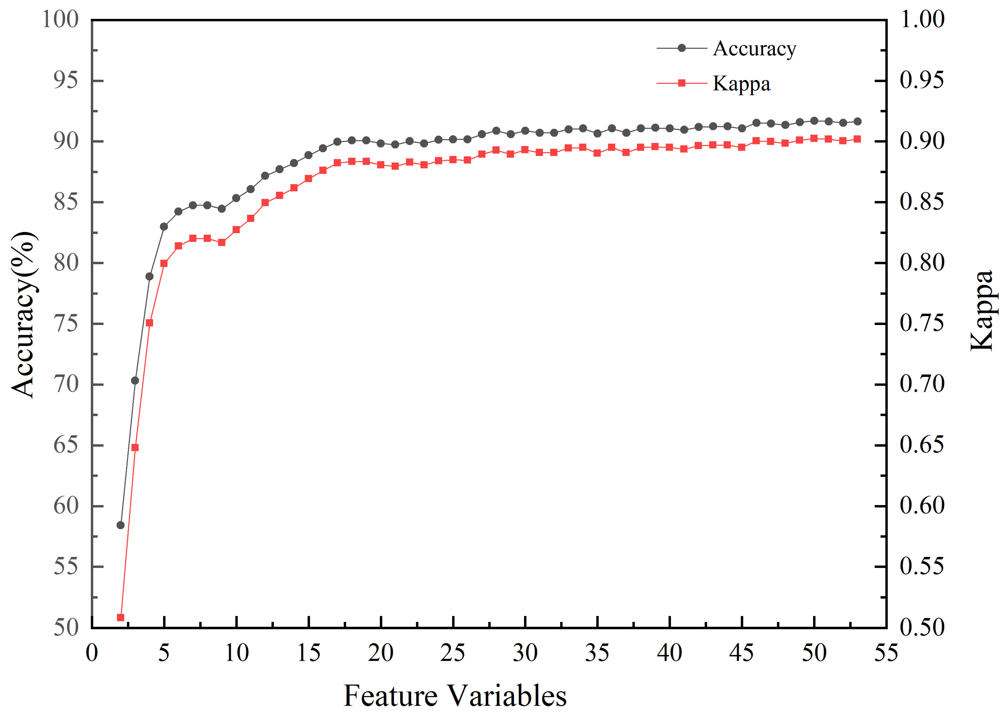
3.4. Analysis of Recursive Feature Elimination Results

In this study, a total of 53 features were extracted, and each of them contributed differently to the vegetation classification results. The RFE algorithm was performed to sort the importance of each feature. As shown in Figure 4, the overall accuracy and the kappa coefficient improved significantly with the increase in feature variables. When the number of feature variables was 20, the overall accuracy was 89.84% (85.02%–94.66%, 95% confidence interval) and the kappa coefficient was 0.88. When the number of feature variables exceeded 20, the curve showed a slight fluctuation trend first and then tended to be stable. When the number of feature variables reached 36, the overall accuracy was 91.06% (85.59%–96.53%, 95% confidence interval) and the kappa coefficient was 0.90. After that, the continuous increase in feature variables could not improve the overall accuracy significantly. This indicates that an excessive number of features causes data redundancy and over-fitting, thus affecting the accuracy of the classifier.

According to the result of RFE, the top 36 important features were determined as the optimal feature subset for wetland vegetation classification. As shown in

Table 6. Optimized feature subset and feature importance ranking.

Feature Ranking	Feature Name	Feature Ranking	Feature Name	Feature Ranking	Feature Name
1	Mean DSM	13	Standard deviation b	25	GLCM_Ent r
2	GLCM_Hom g	14	GLCM_StdDev g	26	GLCM_Ent g
3	GLCM_Hom r	15	NGRDI	27	Standard deviation DSM
4	COM2	16	ExG	28	GLCM_StdDev r
5	NGBDI	17	RGRI	29	Area
6	GLCM_Hom b	18	Standard deviation G	30	GLCM_StdDev b
7	VEG	19	Standard deviation R	31	GLCM_Dis g
8	BGRI	20	GLCM_ASM r	32	GLCM_Dis r
9	VDVI	21	CIVE	33	COM
10	WI	22	GLCM_Ent b	34	GLCM_Cor g
11	RGBRI	23	GLCM_ASM b	35	Shape index
12	RGBVI	24	GLCM_ASM g	36	Mean B

, thirteen VIs, fifteen texture features, four spectral features, two geometric features, and two height features were selected from the original 53 features. The importance of height information (DSM) ranked first, and the homogeneity derived from green, red and blue bands were second, third and sixth, respectively. The results indicate that height information is of great significance and becomes the primary feature to discriminate wetland vegetation at the species level, due to the relative similarity of the spectral characteristics. Al-Najjar et al. [58] demonstrated that height information can ameliorate differences between vegetation, especially in dense vegetation areas. Cao et al. [47] also demonstrated the effectiveness of height information in the classification of mangrove species. Most vegetation indices also played an important role in classification, and most of them ranked within the top ten, such as COM2, NGBDI, VEG, BGRI, VDVI, and WI. Vegetation indices are used as predictors in many studies that use UAVs equipped with RGB cameras, such as Phragmites australis and mangrove mapping [27,47], wetland vegetation classification [38,48], crop mapping [86], mangrove and marsh vegetation biomass retrieval [87,88], coastal wetland restoration [89], and estimating the potassium (K) nutritional status of rice [90]. These studies have highlighted the high application value of vegetation indices. At the same time, texture features effectively compensate for the lack of spectral information [56], and also play an auxiliary role in wetland vegetation classification. In our study, 15 texture features were chosen by the RFE algorithm, with only five ranking among the top twenty. Pena et al. [53] also stated that the contribution of vegetation indices to the crop classification model was much higher than that of texture features, although texture features were necessary in crop classification. Compared with other features, the contribution of geometric features was significantly slight, and only area and shape index were selected by the RFE algorithm, ranking 29 and 35, respectively. Yu et al. [61] pointed out that the gaps and textures in high-resolution images caused the objects to have no obvious geometric pattern, so geometric features could not become the dominant feature to identify wetland vegetation. Specifically, wetland vegetation is affected by water levels, climate, soil, and other factors. The existing forms and growth conditions of vegetation in the same region are diverse; therefore, it is difficult for geometric features to discriminate wetland vegetation independently. In our study, some Zizania latifolia were affected by Alternanthera philoxeroides, and they were mixed in other vegetations in the form of lodging, showing morphological differences to the normal growth of Zizania latifolia. Therefore, the pattern of the generated objects showed a large difference in the same type of vegetation.

3.5. Analysis of the Effectiveness of Feature Selection

Comparing scenario 5 and 10 (Table 5), the overall accuracy of RF-RFE was 90.73%, which was 0.97% higher than that of RF based on the 53 original features. The confusion matrix showed that RF-RFE successfully reduced the misclassification and omission between vegetation species. The PA and UA of Sambucus chinensis were 100% and 96.97%, respectively, which were 3.12% and 0.09% higher than those in scenario 5. Similarly, feature selection also improved the UA of Zizania latifolia, Phragmites australis, Alternanthera philoxeroides, and Sambucus chinensis. Although RF-RFE provided a lower PA of 71.43% for tree shrubs than that in scenario 5, with a PA of 73.68%, RF-RFE was an optimal classification model for the differentiation of all vegetation species.

The results showed that the combination of multi-features can greatly improve the classification accuracy, but high-dimensional features will reduce the classification model efficiency. Feature selection is capable of screening out the best feature subset, which is an indispensable step to classify wetland vegetation by multi-features. Zuo et al. [48] designed 12 groups of comparative experiments using different feature combinations during marsh vegetation mapping, and they verified that the classification accuracy after RFE feature selection was higher than without feature selection. Zhou et al. [79] also showed that the RFE feature selection algorithm can select the most favorable features for forest stand classification, successfully improving the classification accuracy from 80.57% to 81.05%. Previous studies have also demonstrated the advantages of the RFE feature selection method in many research areas [41,91,92,93], such as agricultural pattern recognition, mangrove species classification, and landslide susceptibility mapping. Using high-resolution remote sensing images to monitor and map wetland vegetation is becoming more common, and the RF-RFE model is a promising method for wetland vegetation classification.

3.6. Comparison of Object-Based Classification Results

The object-based classification results of ten object-based classification scenarios are presented in Figure 5. The classification maps of scenario 2 and scenario 6 had the worst classification effect, with many misclassifications. Based on the field survey, the vegetation distribution of the other eight scenarios is nearly consistent with the original image. The RF-RFE model has the best classification effect, and is effective at distinguishing Nelumbo nucifera, Zizania latifolia, and dead plants in the southwestern portion of the study area.

Our study shows that UAV-based RGB imagery has great potential in wetland vegetation classification. One key advantage of high-resolution UAV imagery is that the data collection is much more flexible and cost efficient. Additionally, it can provide massive shape, geometry and texture features to make up for the lack of spectral information, allowing high-accuracy classification to be achieved in this complex wetland environment. Combining the OBIA method with machine learning algorithms is a promising way to achieve high-precision wetland vegetation classification at the species level, and the RFE feature selection method is an important step to improve the accuracy of the classifier. Our results provide a basis for monitoring and mapping wetland vegetation in an efficient and economical way.

Although object-based wetland vegetation classification produces a good result using RF-RFE, some limitations remain. Firstly, previous studies pointed out that the accuracy of the vegetation classification varied seasonally [94]; therefore, the feasibility of the method applied in this paper remains to be explored for other seasons. Secondly, emerging machine learning algorithms still have some issues [95]. The classification model parameters were fixed in this study. Optimizing the model parameters, or combining different classifiers together, is a practicable way to achieve improved classification results in a complex wetland environment. Zhang et al. [40] produced both community- and species-level classifications of object-based marsh vegetation, combining SVM, RF, and minimum noise fraction, with an overall accuracy of over 90%. Zhang et al. [96] showed that there are no perfect image classifiers and different classifiers may complement each other, and their results showed that the integration of classifiers provided more accurate vegetation identification than a single classifier. Hao et al. [97] also found that single classifiers and hybrid classifiers performed differently under different conditions. Specifically, hybrid classifiers performed better with a small training sample, and a single classifier achieved good performance with abundant training samples. Furthermore, high-resolution images result in a huge amount of data with longer computing times. The development of an efficient and universal classification model based on UAV-based RGB imagery, which could be implemented with less professional expertise, is the focus of our future research, as it would contribute to vegetation monitoring and mapping of inaccessible wetlands. The contribution of additional features and feature selection methods can also be evaluated and assessed in future work.

4. Conclusions

In this study, we evaluated the feasibility of using UAV-based RGB imagery for wetland vegetation classification at the species level. OBIA technology was employed to overcome the limitation of traditional pixel-based classification methods. After multi-feature extraction and selection, we designed ten scenarios to compare the contributions of five machine learning algorithms, multi-feature combinations, and feature selections to the classification results. The optimal configuration for wetland vegetation classification was selected based on the overall accuracy, kappa coefficient, PA, and UA. Based on the analysis of ten scenarios, the following conclusions could be drawn:

(1)

When object-based wetland vegetation classification was carried out with all the original features, RF performed better than Bayes, KNN, SVM, and DT.

(2)

Multi-feature combination can help UAV-based RGB imagery realize wetland vegetation classification. Different types of features contributed unequally to the classifier. Owing to the similarity of the spectral information in wetland vegetation, height information became the primary feature discriminating wetland vegetation. The contribution of vegetation indices to wetland vegetation classification was irreplaceable, and texture features were less important than vegetation indices, but still indispensable.

(3)

The classification effect of RF-RFE was the best among the ten scenarios. Feature selection is an effective way to improve the performance of the classifier. A large number of features of redundant or irrelevant information negatively affects the classification. The RFE feature selection algorithm can effectively select the best feature subset to improve the classification accuracy.

This paper demonstrates that UAVs with RGB cameras have the advantages of stronger operability, higher universality, and lower cost, which make them a powerful platform for wetland vegetation monitoring and mapping. The UAV images with high temporal and spatial resolution provide rich image features that can be used to produce wetland vegetation classification at the species level, overcoming the difficulties of traditional wetland vegetation surveys. The method proposed in this paper is more convenient to implement from data acquisition to data processing, simultaneously achieving rapid and high-precision wetland vegetation mapping without the sufficient professional background knowledge of relevant personnel. The approach presented in this paper can be applied to execute long-term and accurate dynamic monitoring of wetland vegetation.

References

1. Zedler, J.B.; Kercher, S. Wetland resources: Status, trends, ecosystem services, and restorability. Annu. Rev. Environ. Resour. 2005, 30, 39–74. [Google Scholar] [CrossRef] [Green Version]
2. Zhang, Y.L.; Lu, D.S.; Yang, B.; Sun, C.H.; Sun, M. Coastal wetland vegetation classification with a landsat thematic mapper image. Int. J. Remote Sens. 2011, 32, 545–561. [Google Scholar] [CrossRef]
3. Taddeo, S.; Dronova, I. Indicators of vegetation development in restored wetlands. Ecol. Indic. 2018, 94, 454–467. [Google Scholar] [CrossRef]
4. Adam, E.; Mutanga, O.; Rugege, D. Multispectral and hyperspectral remote sensing for identification and mapping of wetland vegetation: A review. Wetl. Ecol. Manag. 2010, 18, 281–296. [Google Scholar] [CrossRef]
5. Adeli, S.; Salehi, B.; Mahdianpari, M.; Quackenbush, L.J.; Brisco, B.; Tamiminia, H.; Shaw, S. Wetland monitoring using sar data: A meta-analysis and comprehensive review. Remote Sens. 2020, 12, 2190. [Google Scholar] [CrossRef]
6. Boon, M.A.; Greenfield, R.; Tesfamichael, S. Wetland assessment using unmanned aerial vehicle (uav) photogrammetry. In Proceedings of the 23rd Congress of the International-Society-for-Photogrammetry-and-Remote-Sensing (ISPRS), Prague, Czech Republic, 12–19 July 2016; pp. 781–788. [Google Scholar]
7. Guo, M.; Li, J.; Sheng, C.L.; Xu, J.W.; Wu, L. A review of wetland remote sensing. Sensors 2017, 17, 777. [Google Scholar] [CrossRef] [PubMed] [Green Version]
8. Lane, C.R.; Liu, H.X.; Autrey, B.C.; Anenkhonov, O.A.; Chepinoga, V.V.; Wu, Q.S. Improved wetland classification using eight-band high resolution satellite imagery and a hybrid approach. Remote Sens. 2014, 6, 12187–12216. [Google Scholar] [CrossRef] [Green Version]
9. Martinez, J.M.; Le Toan, T. Mapping of flood dynamics and spatial distribution of vegetation in the amazon floodplain using multitemporal sar data. Remote Sens. Environ. 2007, 108, 209–223. [Google Scholar] [CrossRef]
10. Pengra, B.W.; Johnston, C.A.; Loveland, T.R. Mapping an invasive plant, phragmites australis, in coastal wetlands using the eo-1 hyperion hyperspectral sensor. Remote Sens. Environ. 2007, 108, 74–81. [Google Scholar] [CrossRef]
11. Wright, C.; Gallant, A. Improved wetland remote sensing in yellowstone national park using classification trees to combine tm imagery and ancillary environmental data. Remote Sens. Environ. 2007, 107, 582–605. [Google Scholar] [CrossRef]
12. Hess, L.L.; Melack, J.M.; Novo, E.; Barbosa, C.C.F.; Gastil, M. Dual-season mapping of wetland inundation and vegetation for the central amazon basin. Remote Sens. Environ. 2003, 87, 404–428. [Google Scholar] [CrossRef]
13. Belluco, E.; Camuffo, M.; Ferrari, S.; Modenese, L.; Silvestri, S.; Marani, A.; Marani, M. Mapping salt-marsh vegetation by multispectral and hyperspectral remote sensing. Remote Sens. Environ. 2006, 105, 54–67. [Google Scholar] [CrossRef]
14. Lu, B.; He, Y.H. Species classification using unmanned aerial vehicle (uav)-acquired high spatial resolution imagery in a heterogeneous grassland. ISPRS-J. Photogramm. Remote Sens. 2017, 128, 73–85. [Google Scholar] [CrossRef]
15. Ruwaimana, M.; Satyanarayana, B.; Otero, V.; Muslim, A.M.; Syafiq, A.M.; Ibrahim, S.; Raymaekers, D.; Koedam, N.; Dahdouh-Guebas, F. The advantages of using drones over space-borne imagery in the mapping of mangrove forests. PLoS ONE 2018, 13, e0200288. [Google Scholar] [CrossRef] [PubMed] [Green Version]
16. Zhang, S.M.; Zhao, G.X.; Lang, K.; Su, B.W.; Chen, X.N.; Xi, X.; Zhang, H.B. Integrated satellite, unmanned aerial vehicle (uav) and ground inversion of the spad of winter wheat in the reviving stage. Sensors 2019, 19, 1485. [Google Scholar] [CrossRef] [PubMed] [Green Version]
17. Anderson, K.; Gaston, K.J. Lightweight unmanned aerial vehicles will revolutionize spatial ecology. Front. Ecol. Environ. 2013, 11, 138–146. [Google Scholar] [CrossRef] [Green Version]
18. Berni, J.A.J.; Zarco-Tejada, P.J.; Suarez, L.; Fereres, E. Thermal and narrowband multispectral remote sensing for vegetation monitoring from an unmanned aerial vehicle. IEEE Trans. Geosci. Remote Sens. 2009, 47, 722–738. [Google Scholar] [CrossRef] [Green Version]
19. Matese, A.; Toscano, P.; Di Gennaro, S.F.; Genesio, L.; Vaccari, F.P.; Primicerio, J.; Belli, C.; Zaldei, A.; Bianconi, R.; Gioli, B. Intercomparison of uav, aircraft and satellite remote sensing platforms for precision viticulture. Remote Sens. 2015, 7, 2971–2990. [Google Scholar] [CrossRef] [Green Version]
20. Joyce, K.E.; Anderson, K.; Bartolo, R.E. Of course we fly unmanned-we’re women! Drones 2021, 5, 21. [Google Scholar] [CrossRef]
21. Diez, Y.; Kentsch, S.; Fukuda, M.; Caceres, M.L.L.; Moritake, K.; Cabezas, M. Deep learning in forestry using uav-acquired rgb data: A practical review. Remote Sens. 2021, 13, 2837. [Google Scholar] [CrossRef]
22. Bendig, J.; Yu, K.; Aasen, H.; Bolten, A.; Bennertz, S.; Broscheit, J.; Gnyp, M.L.; Bareth, G. Combining uav-based plant height from crop surface models, visible, and near infrared vegetation indices for biomass monitoring in barley. Int. J. Appl. Earth Obs. Geoinf. 2015, 39, 79–87. [Google Scholar] [CrossRef]
23. Jiang, X.P.; Gao, M.; Gao, Z.Q. A novel index to detect green-tide using uav-based rgb imagery. Estuar. Coast. Shelf Sci. 2020, 245, 106943. [Google Scholar] [CrossRef]
24. Sugiura, R.; Tsuda, S.; Tamiya, S.; Itoh, A.; Nishiwaki, K.; Murakami, N.; Shibuya, Y.; Hirafuji, M.; Nuske, S. Field phenotyping system for the assessment of potato late blight resistance using rgb imagery from an unmanned aerial vehicle. Biosyst. Eng. 2016, 148, 1–10. [Google Scholar] [CrossRef]
25. Dronova, I.; Kislik, C.; Dinh, Z.; Kelly, M. A review of unoccupied aerial vehicle use in wetland applications: Emerging opportunities in approach, technology, and data. Drones 2021, 5, 45. [Google Scholar] [CrossRef]
26. Bhatnagar, S.; Gill, L.; Ghosh, B. Drone image segmentation using machine and deep learning for mapping raised bog vegetation communities. Remote Sens. 2020, 12, 2602. [Google Scholar] [CrossRef]
27. Corti Meneses, N.; Brunner, F.; Baier, S.; Geist, J.; Schneider, T. Quantification of extent, density, and status of aquatic reed beds using point clouds derived from uav-rgb imagery. Remote Sens. 2018, 10, 1869. [Google Scholar] [CrossRef] [Green Version]
28. Fu, B.L.; Liu, M.; He, H.C.; Lan, F.W.; He, X.; Liu, L.L.; Huang, L.K.; Fan, D.L.; Zhao, M.; Jia, Z.L. Comparison of optimized object-based rf-dt algorithm and segnet algorithm for classifying karst wetland vegetation communities using ultra-high spatial resolution uav data. Int. J. Appl. Earth Obs. Geoinf. 2021, 104, 15. [Google Scholar] [CrossRef]
29. Dragut, L.; Tiede, D.; Levick, S.R. Esp: A tool to estimate scale parameter for multiresolution image segmentation of remotely sensed data. Int. J. Geogr. Inf. Sci. 2010, 24, 859–871. [Google Scholar] [CrossRef]
30. Zheng, Y.H.; Wu, J.P.; Wang, A.Q.; Chen, J. Object- and pixel-based classifications of macroalgae farming area with high spatial resolution imagery. Geocarto Int. 2018, 33, 1048–1063. [Google Scholar] [CrossRef]
31. Estoque, R.C.; Murayama, Y.; Akiyama, C.M. Pixel-based and object-based classifications using high- and medium-spatial-resolution imageries in the urban and suburban landscapes. Geocarto Int. 2015, 30, 1113–1129. [Google Scholar] [CrossRef] [Green Version]
32. Pande-Chhetri, R.; Abd-Elrahman, A.; Liu, T.; Morton, J.; Wilhelm, V.L. Object-based classification of wetland vegetation using very high-resolution unmanned air system imagery. Eur. J. Remote Sens. 2017, 50, 564–576. [Google Scholar] [CrossRef] [Green Version]
33. Abeysinghe, T.; Milas, A.S.; Arend, K.; Hohman, B.; Reil, P.; Gregory, A.; Vazquez-Ortega, A. Mapping invasive phragmites australis in the old woman creek estuary using uav remote sensing and machine learning classifiers. Remote Sens. 2019, 11, 1380. [Google Scholar] [CrossRef] [Green Version]
34. Feng, Q.L.; Liu, J.T.; Gong, J.H. Uav remote sensing for urban vegetation mapping using random forest and texture analysis. Remote Sens. 2015, 7, 1074–1094. [Google Scholar] [CrossRef] [Green Version]
35. Torres-Sanchez, J.; Pena, J.M.; de Castro, A.I.; Lopez-Granados, F. Multi-temporal mapping of the vegetation fraction in early-season wheat fields using images from uav. Comput. Electron. Agric. 2014, 103, 104–113. [Google Scholar] [CrossRef]
36. Blaschke, T. Object based image analysis for remote sensing. ISPRS-J. Photogramm. Remote Sens. 2010, 65, 2–16. [Google Scholar] [CrossRef] [Green Version]
37. Liu, T.; Abd-Elrahman, A.; Morton, J.; Wilhelm, V.L. Comparing fully convolutional networks, random forest, support vector machine, and patch-based deep convolutional neural networks for object-based wetland mapping using images from small unmanned aircraft system. GISci. Remote Sens. 2018, 55, 243–264. [Google Scholar] [CrossRef]
38. Geng, R.F.; Jin, S.G.; Fu, B.L.; Wang, B. Object-based wetland classification using multi-feature combination of ultra-high spatial resolution multispectral images. Can. J. Remote Sens. 2020, 46, 784–802. [Google Scholar] [CrossRef]
39. Cutler, D.R.; Edwards, T.C.; Beard, K.H.; Cutler, A.; Hess, K.T. Random forests for classification in ecology. Ecology 2007, 88, 2783–2792. [Google Scholar] [CrossRef]
40. Zhang, C.Y.; Xie, Z.X. Object-based vegetation mapping in the kissimmee river watershed using hymap data and machine learning techniques. Wetlands 2013, 33, 233–244. [Google Scholar] [CrossRef]
41. Zhou, X.Z.; Wen, H.J.; Zhang, Y.L.; Xu, J.H.; Zhang, W.G. Landslide susceptibility mapping using hybrid random forest with geodetector and rfe for factor optimization. Geosci. Front. 2021, 12, 101211. [Google Scholar] [CrossRef]
42. Balha, A.; Mallick, J.; Pandey, S.; Gupta, S.; Singh, C.K. A comparative analysis of different pixel and object-based classification algorithms using multi-source high spatial resolution satellite data for lulc mapping. Earth Sci. Inform. 2021, 14, 2231–2247. [Google Scholar] [CrossRef]
43. Gibril, M.B.A.; Shafri, H.Z.M.; Hamedianfar, A. New semi-automated mapping of asbestos cement roofs using rule-based object-based image analysis and taguchi optimization technique from worldview-2 images. Int. J. Remote Sens. 2017, 38, 467–491. [Google Scholar] [CrossRef]
44. Qian, Y.G.; Zhou, W.Q.; Yan, J.L.; Li, W.F.; Han, L.J. Comparing machine learning classifiers for object-based land cover classification using very high resolution imagery. Remote Sens. 2015, 7, 153–168. [Google Scholar] [CrossRef]
45. Laliberte, A.S.; Browning, D.M.; Rango, A. A comparison of three feature selection methods for object-based classification of sub-decimeter resolution ultracam-l imagery. Int. J. Appl. Earth Obs. Geoinf. 2012, 15, 70–78. [Google Scholar] [CrossRef]
46. Georganos, S.; Grippa, T.; Vanhuysse, S.; Lennert, M.; Shimoni, M.; Kalogirou, S.; Wolff, E. Less is more: Optimizing classification performance through feature selection in a very-high-resolution remote sensing object-based urban application. GISci. Remote Sens. 2018, 55, 221–242. [Google Scholar] [CrossRef]
47. Cao, J.J.; Leng, W.C.; Liu, K.; Liu, L.; He, Z.; Zhu, Y.H. Object-based mangrove species classification using unmanned aerial vehicle hyperspectral images and digital surface models. Remote Sens. 2018, 10, 89. [Google Scholar] [CrossRef] [Green Version]
48. Zuo, P.P.; Fu, B.L.; Lan, F.W.; Xie, S.Y.; He, H.C.; Fan, D.L.; Lou, P.Q. Classification method of swamp vegetation using uav multispectral data. China Environ. Sci. 2021, 41, 2399–2410. [Google Scholar]
49. Boon, M.A.; Tesfamichael, S. Determination of the present vegetation state of a wetland with uav rgb imagery. In Proceedings of the 37th International Symposium on Remote Sensing of Environment, Tshwane, South Africa, 8–12 May 2017; Copernicus Gesellschaft Mbh: Tshwane, South Africa; pp. 37–41. [Google Scholar]
50. Zhang, T.; Ban, X.; Wang, X.L.; Cai, X.B.; Li, E.H.; Wang, Z.; Yang, C.; Zhang, Q.; Lu, X.R. Analysis of nutrient transport and ecological response in honghu lake, china by using a mathematical model. Sci. Total Environ. 2017, 575, 418–428. [Google Scholar] [CrossRef]
51. Liu, Y.; Ren, W.B.; Shu, T.; Xie, C.F.; Jiang, J.H.; Yang, S. Current status and the long-term change of riparian vegetation in last fifty years of lake honghu. Resour. Environ. Yangtze Basin 2015, 24, 38–45. [Google Scholar]
52. Flanders, D.; Hall-Beyer, M.; Pereverzoff, J. Preliminary evaluation of ecognition object-based software for cut block delineation and feature extraction. Can. J. Remote Sens. 2003, 29, 441–452. [Google Scholar] [CrossRef]
53. Pena-Barragan, J.M.; Ngugi, M.K.; Plant, R.E.; Six, J. Object-based crop identification using multiple vegetation indices, textural features and crop phenology. Remote Sens. Environ. 2011, 115, 1301–1316. [Google Scholar] [CrossRef]
54. Gao, Y.; Mas, J.F.; Maathuis, B.H.P.; Zhang, X.M.; Van Dijk, P.M. Comparison of pixel-based and object-oriented image classification approaches - a case study in a coal fire area, wuda, inner mongolia, china. Int. J. Remote Sens. 2006, 27, 4039–4055. [Google Scholar]
55. Lin, F.F.; Zhang, D.Y.; Huang, Y.B.; Wang, X.; Chen, X.F. Detection of corn and weed species by the combination of spectral, shape and textural features. Sustainability 2017, 9, 1335. [Google Scholar] [CrossRef] [Green Version]
56. Zhang, H.X.; Li, Q.Z.; Liu, J.G.; Du, X.; Dong, T.F.; McNairn, H.; Champagne, C.; Liu, M.X.; Shang, J.L. Object-based crop classification using multi-temporal spot-5 imagery and textural features with a random forest classifier. Geocarto Int. 2018, 33, 1017–1035. [Google Scholar] [CrossRef]
57. Zhang, L.; Liu, Z.; Ren, T.W.; Liu, D.Y.; Ma, Z.; Tong, L.; Zhang, C.; Zhou, T.Y.; Zhang, X.D.; Li, S.M. Identification of seed maize fields with high spatial resolution and multiple spectral remote sensing using random forest classifier. Remote Sens. 2020, 12, 362. [Google Scholar] [CrossRef] [Green Version]
58. Al-Najjar, H.A.H.; Kalantar, B.; Pradhan, B.; Saeidi, V.; Halin, A.A.; Ueda, N.; Mansor, S. Land cover classification from fused dsm and uav images using convolutional neural networks. Remote Sens. 2019, 11, 1461. [Google Scholar] [CrossRef] [Green Version]
59. Meyer, G.E.; Neto, J.C. Verification of color vegetation indices for automated crop imaging applications. Comput. Electron. Agric. 2008, 63, 282–293. [Google Scholar] [CrossRef]
60. Agapiou, A. Vegetation extraction using visible-bands from openly licensed unmanned aerial vehicle imagery. Drones 2020, 4, 27. [Google Scholar] [CrossRef]
61. Yu, Q.; Gong, P.; Clinton, N.; Biging, G.; Kelly, M.; Schirokauer, D. Object-based detailed vegetation classification. With airborne high spatial resolution remote sensing imagery. Photogramm. Eng. Remote Sens. 2006, 72, 799–811. [Google Scholar] [CrossRef] [Green Version]
62. Woebbecke, D.M.; Meyer, G.E.; Vonbargen, K.; Mortensen, D.A. Color indexes for weed identification under various soil, residue, and lighting conditions. Trans. ASAE 1995, 38, 259–269. [Google Scholar] [CrossRef]
63. Guerrero, J.M.; Pajares, G.; Montalvo, M.; Romeo, J.; Guijarro, M. Support vector machines for crop/weeds identification in maize fields. Expert Syst. Appl. 2012, 39, 11149–11155. [Google Scholar] [CrossRef]
64. Guijarro, M.; Pajares, G.; Riomoros, I.; Herrera, P.J.; Burgos-Artizzu, X.P.; Ribeiro, A. Automatic segmentation of relevant textures in agricultural images. Comput. Electron. Agric. 2011, 75, 75–83. [Google Scholar] [CrossRef] [Green Version]
65. Du, M.M.; Noguchi, N. Monitoring of wheat growth status and mapping of wheat yield’s within-field spatial variations using color images acquired from uav-camera system. Remote Sens. 2017, 9, 289. [Google Scholar] [CrossRef] [Green Version]
66. Wan, L.; Li, Y.J.; Cen, H.Y.; Zhu, J.P.; Yin, W.X.; Wu, W.K.; Zhu, H.Y.; Sun, D.W.; Zhou, W.J.; He, Y. Combining uav-based vegetation indices and image classification to estimate flower number in oilseed rape. Remote Sens. 2018, 10, 1484. [Google Scholar] [CrossRef] [Green Version]
67. Calderon, R.; Navas-Cortes, J.A.; Lucena, C.; Zarco-Tejada, P.J. High-resolution airborne hyperspectral and thermal imagery for early, detection of verticillium wilt of olive using fluorescence, temperature and narrow-band spectral indices. Remote Sens. Environ. 2013, 139, 231–245. [Google Scholar] [CrossRef]
68. Xie, B.; Yang, W.N.; Wang, F. A new estimate method for fractional vegetation cover based on uav visual light spectrum. Sci. Surv. Mapp. 2020, 45, 72–77. [Google Scholar]
69. Shiraishi, T.; Motohka, T.; Thapa, R.B.; Watanabe, M.; Shimada, M. Comparative assessment of supervised classifiers for land use-land cover classification in a tropical region using time-series palsar mosaic data. IEEE J. Sel. Top. Appl. Earth Observ. Remote Sens. 2014, 7, 1186–1199. [Google Scholar] [CrossRef]
70. Wieland, M.; Pittore, M. Performance evaluation of machine learning algorithms for urban pattern recognition from multi-spectral satellite images. Remote Sens. 2014, 6, 2912–2939. [Google Scholar] [CrossRef] [Green Version]
71. Murthy, S.K. Automatic construction of decision trees from data: A multi-disciplinary survey. Data Min. Knowl. Discov. 1998, 2, 345–389. [Google Scholar] [CrossRef]
72. Friedl, M.A.; Brodley, C.E. Decision tree classification of land cover from remotely sensed data. Remote Sens. Environ. 1997, 61, 399–409. [Google Scholar] [CrossRef]
73. Apte, C.; Weiss, S. Data mining with decision trees and decision rules. Futur. Gener. Comp. Syst. 1997, 13, 197–210. [Google Scholar] [CrossRef]
74. Cortes, C.; Vapnik, V. Support-vector networks. Mach. Learn. 1995, 20, 273–297. [Google Scholar] [CrossRef]
75. Gxokwe, S.; Dube, T.; Mazvimavi, D. Leveraging google earth engine platform to characterize and map small seasonal wetlands in the semi-arid environments of south africa. Sci. Total Environ. 2022, 803, 12. [Google Scholar] [CrossRef] [PubMed]
76. Breiman, L. Random forests. Mach. Learn. 2001, 45, 5–32. [Google Scholar] [CrossRef] [Green Version]
77. Prasad, A.M.; Iverson, L.R.; Liaw, A. Newer classification and regression tree techniques: Bagging and random forests for ecological prediction. Ecosystems 2006, 9, 181–199. [Google Scholar] [CrossRef]
78. Wang, X.F.; Wang, Y.; Zhou, C.W.; Yin, L.C.; Feng, X.M. Urban forest monitoring based on multiple features at the single tree scale by uav. Urban For. Urban Green. 2021, 58, 10. [Google Scholar] [CrossRef]
79. Zhou, X.C.; Zheng, L.; Huang, H.Y. Classification of forest stand based on multi-feature optimization of uav visible light remote sensing. Sci. Silvae Sin. 2021, 57, 24–36. [Google Scholar]
80. Chandrashekar, G.; Sahin, F. A survey on feature selection methods. Comput. Electr. Eng. 2014, 40, 16–28. [Google Scholar] [CrossRef]
81. Hsu, H.H.; Hsieh, C.W.; Lu, M.D. Hybrid feature selection by combining filters and wrappers. Expert Syst. Appl. 2011, 38, 8144–8150. [Google Scholar] [CrossRef]
82. Wang, A.G.; An, N.; Chen, G.L.; Li, L.; Alterovitz, G. Accelerating wrapper-based feature selection with k-nearest-neighbor. Knowledge-Based Syst. 2015, 83, 81–91. [Google Scholar] [CrossRef]
83. Guyon, I.; Weston, J.; Barnhill, S.; Vapnik, V. Gene selection for cancer classification using support vector machines. Mach. Learn. 2002, 46, 389–422. [Google Scholar] [CrossRef]
84. Mao, Y.; Pi, D.Y.; Liu, Y.M.; Sun, Y.X. Accelerated recursive feature elimination based on support vector machine for key variable identification. Chin. J. Chem. Eng. 2006, 14, 65–72. [Google Scholar] [CrossRef]
85. Griffith, D.C.; Hay, G.J. Integrating geobia, machine learning, and volunteered geographic information to map vegetation over rooftops. ISPRS Int. J. Geo-Inf. 2018, 7, 462. [Google Scholar] [CrossRef] [Green Version]
86. Randelovic, P.; Dordevic, V.; Milic, S.; Balesevic-Tubic, S.; Petrovic, K.; Miladinovic, J.; Dukic, V. Prediction of soybean plant density using a machine learning model and vegetation indices extracted from rgb images taken with a uav. Agronomy 2020, 10, 1108. [Google Scholar] [CrossRef]
87. Morgan, G.R.; Wang, C.Z.; Morris, J.T. Rgb indices and canopy height modelling for mapping tidal marsh biomass from a small unmanned aerial system. Remote Sens. 2021, 13, 3406. [Google Scholar] [CrossRef]
88. Tian, Y.C.; Huang, H.; Zhou, G.Q.; Zhang, Q.; Tao, J.; Zhang, Y.L.; Lin, J.L. Aboveground mangrove biomass estimation in beibu gulf using machine learning and uav remote sensing. Sci. Total Environ. 2021, 781. [Google Scholar] [CrossRef]
89. Dale, J.; Burnside, N.G.; Hill-Butler, C.; Berg, M.J.; Strong, C.J.; Burgess, H.M. The use of unmanned aerial vehicles to determine differences in vegetation cover: A tool for monitoring coastal wetland restoration schemes. Remote Sens. 2020, 12, 4022. [Google Scholar] [CrossRef]
90. Lu, J.S.; Eitel, J.U.H.; Engels, M.; Zhu, J.; Ma, Y.; Liao, F.; Zheng, H.B.; Wang, X.; Yao, X.; Cheng, T.; et al. Improving unmanned aerial vehicle (uav) remote sensing of rice plant potassium accumulation by fusing spectral and textural information. Int. J. Appl. Earth Obs. Geoinf. 2021, 104, 15. [Google Scholar] [CrossRef]
91. Jiang, Y.F.; Zhang, L.; Yan, M.; Qi, J.G.; Fu, T.M.; Fan, S.X.; Chen, B.W. High-resolution mangrove forests classification with machine learning using worldview and uav hyperspectral data. Remote Sens. 2021, 13, 1529. [Google Scholar] [CrossRef]
92. Liu, H.P.; Zhang, Y.X. Selection of landsat8 image classification bands based on mlc-rfe. J. Indian Soc. Remote Sens. 2019, 47, 439–446. [Google Scholar] [CrossRef]
93. Ma, L.; Fu, T.Y.; Blaschke, T.; Li, M.C.; Tiede, D.; Zhou, Z.J.; Ma, X.X.; Chen, D.L. Evaluation of feature selection methods for object-based land cover mapping of unmanned aerial vehicle imagery using random forest and support vector machine classifiers. ISPRS Int. J. Geo-Inf. 2017, 6, 51. [Google Scholar] [CrossRef]
94. Gibson, D.J.; Looney, P.B. Seasonal-variation in vegetation classification on perdido key, a barrier-island off the coast of the florida panhandle. J. Coast. Res. 1992, 8, 943–956. [Google Scholar]
95. Zhang, Q. Research progress in wetland vegetation classification by remote sensing. World For. Res. 2019, 32, 49–54. [Google Scholar]
96. Zhang, X.Y.; Feng, X.Z.; Wang, K. Integration of classifiers for improvement of vegetation category identification accuracy based on image objects. N. Z. J. Agric. Res. 2007, 50, 1125–1133. [Google Scholar] [CrossRef]
97. Hao, P.Y.; Wang, L.; Niu, Z. Comparison of hybrid classifiers for crop classification using normalized difference vegetation index time series: A case study for major crops in north xinjiang, china. PLoS ONE 2015, 10, e0137748. [Google Scholar] [CrossRef]
Figure 1. Research area in the Honghu Lake wetland. (a) Location of the Honghu Wetland Nature Reserve in Hubei Province, China (upper left); extent of the study area in Honghu as shown by a Sentinel-2 image and marked in yellow (in the lower left); (b) location of 205 verification samples in the study area as shown by UAV-based RGB images.
Remotesensing 13 04910 g001
Figure 2. Workflow for object-based wetland vegetation classification using the multi-feature selection of UAV-based RGB imagery. DOM: digital orthophoto map; DSM: digital surface model; RGB: red, green and blue; KNN: K-nearest neighbor; SVM: support vector machine; DT: decision tree; RF: random forest; RF-RFE: random forest based on recursive feature elimination algorithm.
Remotesensing 13 04910 g002
Figure 3. Image segmentation using different parameter combinations (scale, shape index and compactness). (a) Image segmentation results with a fixed scale (100), compactness (0.5) and variable shape index; (b) image segmentation results with a fixed scale (100), shape index (0.1) and variable compactness; (c) image segmentation results with a fixed shape index (0.1), compactness (0.5) and variable scale.
Remotesensing 13 04910 g003
Figure 4. Change in the overall accuracy and the kappa coefficient as a function of different feature subsets.
Remotesensing 13 04910 g004
Figure 5. Object-based wetland vegetation classification map.
Remotesensing 13 04910 g005