Abstract
Aquatic reed beds provide important ecological functions, yet their monitoring by remote sensing methods remains challenging. In this study, we propose an approach of assessing aquatic reed stand status indicators based on data from the airborne photogrammetric 3K-system of the German Aerospace Center (DLR). By a Structure from Motion (SfM) approach, we computed stand surface models of aquatic reeds for each of the 14 areas of interest (AOI) investigated at Lake Chiemsee in Bavaria, Germany. Based on reed heights, we subsequently calculated the reed area, surface structure homogeneity and shape of the frontline. For verification, we compared 3K aquatic reed heights against reed stem metrics obtained from ground-based infield data collected at each AOI. The root mean square error (RMSE) for 1358 reference points from the 3K digital surface model and the field-measured data ranged between 39 cm and 104 cm depending on the AOI. Considering strong object movements due to wind and waves, superimposed by water surface effects such as sun glint altering 3K data, the results of the aquatic reed surface reconstruction were promising. Combining the parameter height, area, density and frontline shape, we finally calculated an indicator for status determination: the aquatic reed status index (aRSI), which is based on metrics, and thus is repeatable and transferable in space and time. The findings of our study illustrate that, even under the adverse conditions given by the environment of the aquatic reed, aerial photogrammetry can deliver appropriate results for deriving objective and reconstructable parameters for aquatic reed status (Phragmites australis) assessment.
1. Introduction
Aquatic reed beds are of major importance for freshwater lake ecosystems in Europe. Extensive damage, and thus large declines over numerous Central European lakes, have been reported [1,2,3,4,5,6]. The reasons for this downtrend are manifold. Possible causes include extreme floods, especially during the early growing stages of aquatic reeds [7,8], water level changes, temperature alterations, shore erosion [2], mechanical destruction by ship waves, drifting wood and recreational activities [9], as well as grazing by water birds and introduced species such as muskrats [2,10]. Global warming effects superimpose these threats due to associated shifts in the vegetation period and extreme weather events such as heavy rainfall and thunderstorms. Given the important functions of reed beds and their observed declines, monitoring at a high temporal and spatial resolution is key to better understanding the factors of decline, and to deduce conservation measures. Traditionally, the mapping and status assessment of reed stands is mostly based on visual field assessments by experts, which is costly and time-consuming. Therefore, it is often supported by interpretations of aerial true color to color infrared (CIR) images [3,7,8,11].
For instance, the currently applied reed stand mapping instruction of the Bavarian nature conservation authority is based on the visual assessment of ‘vitality’ by expert opinion and subjective criteria such as ‘greenness’ of reed stands, density or fragmentation of the reed front, etc. [12]. These methods are not only time consuming, but also subject to individual variation. For instance, a classification in dense (healthy) and sparse, suspected die-back patches is hard to perform and often inaccurate [13], the qualitative categorization in ‘vitality’ classes is subjective, expert-dependent and not transferable in space and time. Moreover, the personnel and financial expenses are high, hindering frequent survey intervals.
Consequently, experts suggest digital remote sensing (RS)-based methods as an alternative to classic field surveys. Recent developments in RS sensor systems and analysis methods provide new opportunities for more accurate and less time-consuming monitoring concepts. Considering analyses of long-term trends, RS data are considered as time documents and may be reanalyzed once new methodologies arise.
Recent studies gave promising results in mapping wetland vegetation with modern remote sensing methodologies. For instance, hyperspectral data from the AVIRIS platform was used for the mapping of marshland vegetation [14]. Andresen et al. [15] analyzed Ikonos VHR satellites, CASI hyperspectral airborne and orthophoto data employing object-oriented (OBIA) classification approaches with the aim of monitoring reed and wetland. Villa et al., in several studies, showed [16,17,18] the potential of remote sensing for monitoring aquatic vegetation such as aquatic Phragmites australis with multispectral data. Gilmore et al. [19] used satellite imagery, top of the canopy LiDAR and field spectral data in a multi-temporal, object-based classification approach to distinguish between Phragmites australis, Spartina patens and Typha spp. Samiappan et al. [20] classified reeds (Phragmites australis) in the Gulf of Mexico. They reported an overall accuracy (OA) of 91%, interpreting multispectral sensor data taken from a small unmanned aerial vehicle (UAV) through pixel-based classification with Support Vector Machines along with vegetation indices, morphological attribute profiles and digital surface models. Declining wetland vegetation dominated by Typha sp., Carex sp. and Phragmites australis were mapped and classed into four categories (healthy, stressed, ruderal, die-back) with Airborne Laser Scanning (ALS) data with an OA of 82.5% by Zlinsky et al. [21].
In the recent years, photogrammetry has been competing with Light Detection and Ranging (LiDAR) when it comes to the estimation of vertical structure extents [22]. However, in case of aquatic reed monitoring, few case studies are published using photogrammetric approaches to derive reed heights [23]. Still, this approach is widely used in other domains, e.g., in the field of precision farming. These studies can be seen as comparable to our investigation because of the similar range of plant heights and the canopy structures of agricultural crops and reed (between 1–6 m). Bendig et al. [24] describe the generation of crop surface models of barley with very-high-resolution UAV data from 30 m above ground. For the calculation of the plant heights, a SfM approach was used. Being interested in the performance of the height determination by SfM techniques and aware of the complex surface, they used the heights of rectangular test targets, so called Peli cases, for the accuracy assessment of their models, but not the measured heights of the plants. Accordingly, they reported a mean height difference of 0.01 m. Geipel et al. [25] tested the combination of spectral information from a consumer camera mounted on a hexacopter and derived plant heights from SfM crop surface models. The vertical RMSE for their model ranged from 0.273 m to 0.379 m. A height estimation from SfM of UAV data was also researched for sugar cane plots [26], which are quite similar to reed stands in their vertical extent, as well as in geometric structure. RMSE for data recorded from 200 m above ground level (a.g.l.) range between 0.40 m and 0.57 m. Nonetheless, conditions in agricultural patches are relatively homogenous and stable, which is in contrast to the conditions given by natural aquatic reed beds with their inhomogeneous environmental surroundings, wind-exposed position and the different effects of water surface superimposing the reflected signal. Recently, few studies were conducted with either LiDAR- or SfM-based methodologies under these diverse environmental conditions. Corti et al. [27] evaluated airborne Green-LiDAR data for mapping extent, height and density of aquatic reed beds. Aside from this active remote sensing technology, they tested various SfM methods for modelling the structure and status of aquatic Phragmites australis [23,28]. Here, the RMSE for height reconstruction over reed beds ranged between 1.05 m (rotary wing UAV) and 1.42 m (fixed wing UAV). Moreover, aside from reed height, reed extent and reed density, Corti et al. proposed the reed frontline geometry metric sinuosity as a health status indicator of the aquatic reed stand [23]. Recently, Koma et al. [29] showed the potential of airborne LiDAR to measure reed heights, LAI and biomass from the 3D structure of the vegetation across three Hungarian lakes.
We found no published studies that investigated the possibilities of a multi-camera-array mounted on an airplane for crop surface models or, even further, of surface models of reed stands. Multiple cameras mounted at different angles could further improve SfM 3D reconstruction accuracy compared to single-camera systems.
In our case, we targeted an approach that made the estimation of reed heights the primary information from 3K SfM-processed data. The concept of the airborne 3K system was mainly developed for acquiring data used in the civil sector, such as traffic applications and the airborne monitoring of disaster situations [30,31,32]. With its very high spatial resolution of 0.14 m [33] at 1000 m a.g.l., and three cameras observing objects from different angles, the system seems capable of the 3D modelling of wetland vegetation, and in our case, aquatic reeds. In our concept, reed heights derived from 3K data are the main primary information source for the status assessment of aquatic reeds.
The main aim of our study was to develop an objective method of reed status assessment, based on repeatable and re-constructible automatic processing chains transferable in space (site) and time (monitoring cycles). Our research hypothesis was that metrics derived from reed height models, such as area, canopy surface heterogeneity and frontline structure, allowed an objective and re-constructible reed status assessment.
2. Materials and Methods
2.1. Study Area
The study site is located at Lake Chiemsee in Upper Bavaria, Germany. The origin of the area, located about 80 km southeast of Munich, as with most Bavarian lakes, is ascribable to the last ice age. After Lake Constance (536.0 km2) and Lake Müritz (112.6 km2), Lake Chiemsee with 79.9 km2 is the third-largest lake in Germany (Nixdorf et al., 2004). At Lake Chiemsee, where water level has been regulated in the 17th and 18th century, the development of aquatic reed beds can be easily traced back to 1904, when the water level was lowered by about 0.7 m for land reclamation. The mean water level of the last ten years was calculated to be 518.20 m above sea level. The delta of its largest inflow, the Tiroler Ache, is one of the last intact inland deltas in Central Europe and was declared a nature reserve in 1954. In 1967, the entire lake, as well as the adjacent shores, received the status of a protected landscape. In addition, Lake Chiemsee holds the status of a Ramsar area, i.e., an area of considerable importance for numerous breeding birds and wintering waterbirds (Grosser et al., 1997). The aquatic reed beds at Lake Chiemsee declined by approximately 50% between 1957 and 1991 (Grosser et al., 1997), were stable until 1998 (Hoffmann and Zimmermann, 2000), and seemed to decline again by 12% until 2015, as identified in our internal preparatory studies. The area was predestined for this study because of the still-large and -pure reed populations and the need for monitoring their development under climate change conditions and increasing human pressures.
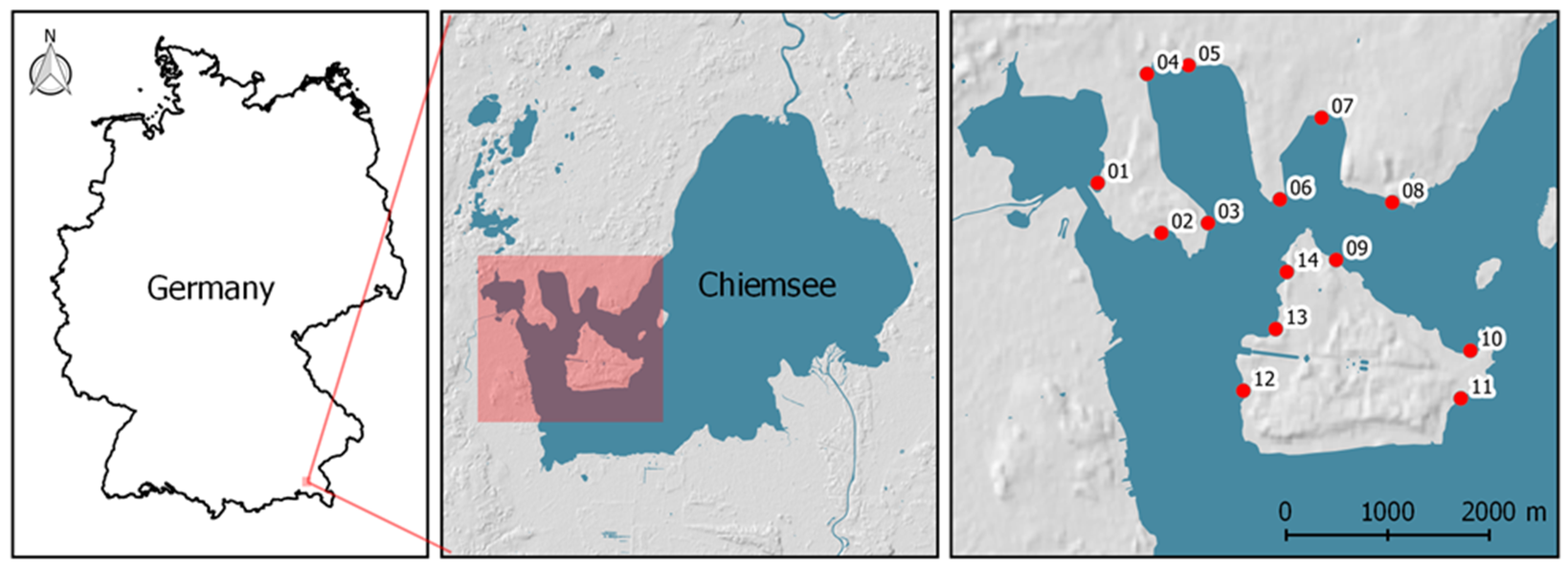
According to Hoffmann and Zimmermann (2000), representative populations of aquatic reeds are located in the northwestern part of the lakeshore and around the island of Herreninsel. Consequently, we decided to focus our surveys on this region. For field measurements, we selected 14 Areas of Interest (AOI), covering both conservational areas and areas with strong anthropogenic influence (Figure 1). The selected AOIs cover the complete diversity range between vital dense and sparse reed stocks.

Figure 1.
(Center): Study area at Lake Chiemsee, Germany (Left), with position of AOIs (Right).
2.2. Field Data Collection
We planned the field survey campaign in early September 2015, as close as possible to the scheduled date of the flight campaign. The field campaign was conducted from 1 September to 15 September 2015.
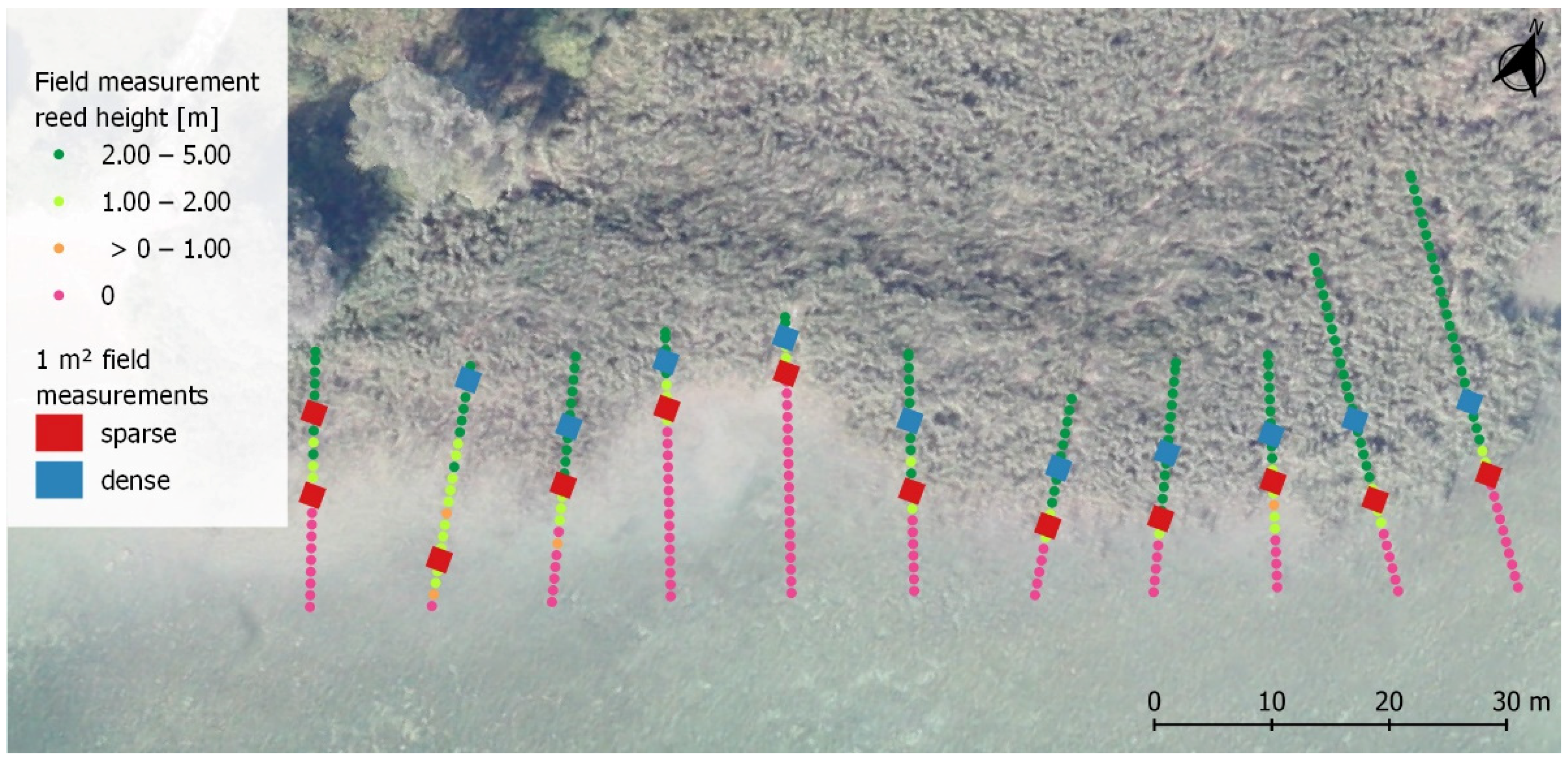
With our sampling design (Figure 2), we accounted for the typical height zonation of the reed beds parallel to the shoreline. At every AOI, we established a one-hundred-meter-long line (exception at AOI 7: 70 m line) parallel to the shoreline. From this line, we laid a perpendicular transect every 10 m starting from the waterside to the shoreline at the day of sampling. At every meter along a transect, we measured water depths and reed stem heights (from the bottom to the top of the reed flower) with a folding rule (to the closest 1 cm). In addition, along each transect we placed two 1 m2 plots in sparse and dense reed zones. Within these defined square plots, we measured stems per m2, number of stems with shoots and the amount of green and dead (i.e., brown) stems, and recorded other biotic (feeding damage by water birds and muskrats) or abiotic damages by driftwood, wind and waves. Driftwood or even larger groups of garbage typically remain stuck in the reed structure. The degree of damage from such objects worsens typically with higher wind speeds. Moreover, wind and waves alone are able to break reed stems or even lay down whole reed stands. The positions of transect endpoints (reference points) were determined using a Trimble GTX DGPS along with a Hurricane antenna. The final accuracy post processing of GPS data was conducted with the software, Trimble Pathfinder Office. Differential correction resulted in a total mean horizontal precision of 46.5 cm for the points. Being aware of the instability of the upper reed surface, which is affected by wind, waves, etc., we based our height and density calculations on 1 m2 raster cells. Therefore, we assumed that the horizontal and height precision was acceptable for a continuously changing surface.
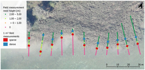
Figure 2.
Schematic of the field survey, determining reed stem heights at every meter in each transect at AOI-06 on top of 3K-Orthomosaic.
2.3. K System and Data Set
The photogrammetric model for the investigated reed stand was calculated based on the data of the photogrammetric 3K system, developed and operated by the German Aerospace Center (DLR) [32]. The DLR 3K system consists of three Canon EOS 1Ds Mark II DLSR cameras, integrated into a ZEISS aerial camera mount. With two sideward-looking cameras with a tilt angle of 35° and one nadir-looking camera, the system covers a swath width of 2.8 km at the flown altitude of 1000 m a.g.l. This results in a pixel size of 0.14 m [33]. The in-flight image overlap for each of the three cameras was 80%; the side overlap was 30%.
The 3K data set was recorded on 21 September 2015 between 11:25 and 12:04 (UTC) from an average flying height of 1000 m a.g.l. The data set comprises 1716 single images provided in JPEG format with attached corresponding navigation parameters from the aircraft internal measurement unit (IMU) in text format.
Water levels of Lake Chiemsee are measured daily by the Bavarian Agency of the Environment [34]. For the day of the data collection, water level was measured with 517.93 m a.s.l.
2.4. Photogrammetric Processing Chain
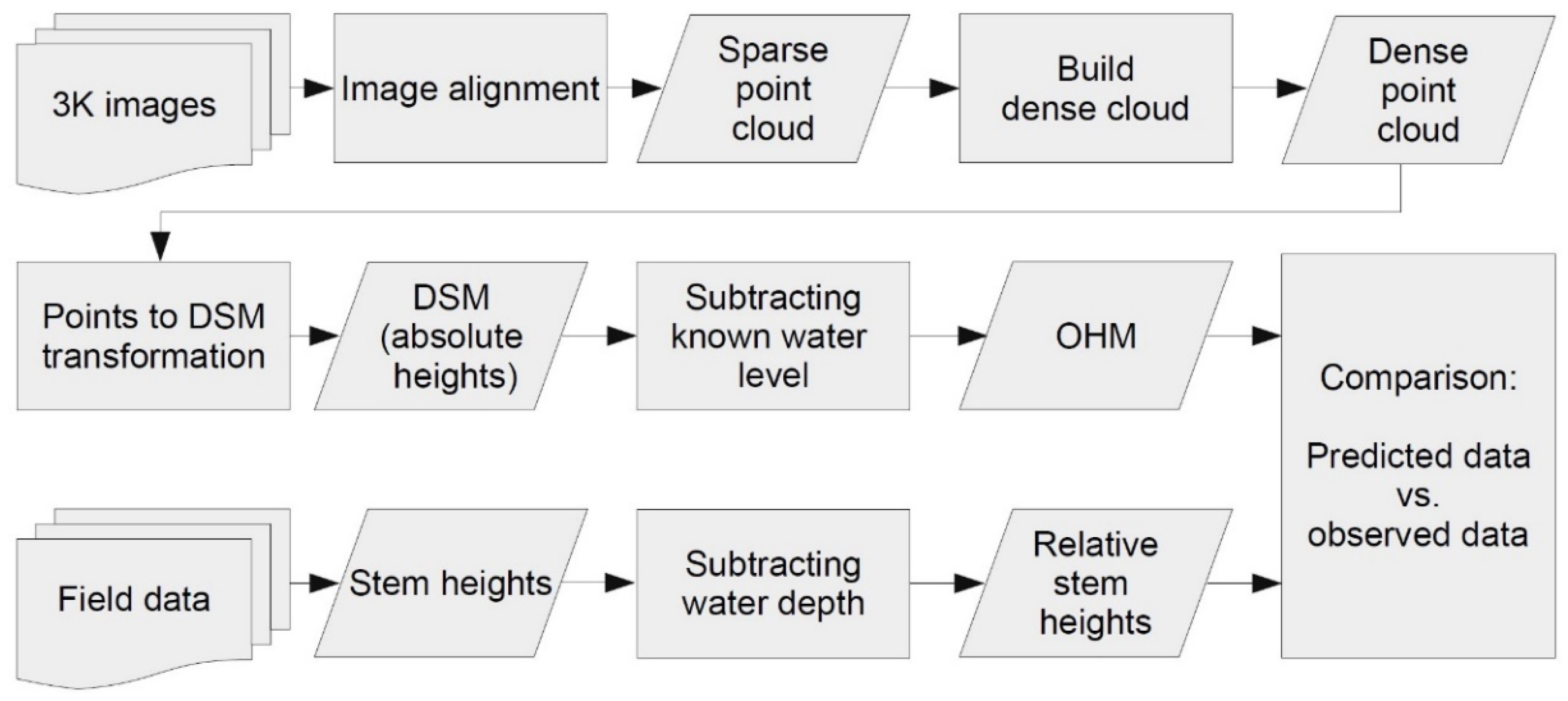
An overview of the photogrammetric processing chain is given in Figure 3. After computing the remote sensing data in the photogrammetric processing chain (image alignment, build dense cloud, points to digital surface model (DSM), calculation of object height mode (OHM)), the results of the predicted reed stem heights (after subtracting known water level) from the model were compared to the field-observed stem heights.
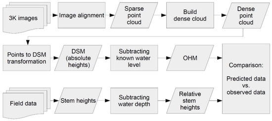
Figure 3.
Flowchart of the photogrammetric processing chain and accuracy assessment for estimating reed stem heights.
For photogrammetric modelling, we used the software Agisoft Photoscan Professional in Version 1.2.6. Agisoft Photoscan (since 2019 called Metashape), which is a common commercial software used by similar projects in the agricultural and forest sectors; it proved to deliver sufficient levels of accuracy [35,36,37]. The following processing chain settings are the results of internal tests to optimize the tradeoff between computation time and modeling accuracy. Accordingly, for each AOI, we started a separate computation. The SfM process starts with the image alignment, generating a sparse point cloud. Position data from the aircrafts GNSS and an inertial measurement unit (IMU) support this process. We selected the settings ‘highest possible accuracy’ and ‘pair preselection’ from the reference IMU data. We set the ‘key point limit’ to 150,000 points and the ’tie point limit’ to an unlimited number of points. The next step was to generate a dense point cloud out of the sparse point cloud from the alignment process. The quality parameter was set to ‘ultra-high’ and the depth filtering to ‘mild’ in order to prevent the software from cutting off stem height outliers in the modelling process. For assuring reproducible results, we did not edit the dense point cloud manually (e.g., cutting outliers). For the following processing steps, we transformed and exported the data as digital surface models (DSM) and orthomosaics (0.136 m resolution) in GeoTiff format.
2.5. Derivation of Aquatic Reed Status Diagnostic Parameters
The applied method for deriving aquatic reed status diagnostic parameters was based on the workflow presented in Corti et al. [23]. Different to that study, which used the OPALS software package, we analyzed the 3K data with the open-source software, QGIS (version 3.16) [38]. As a diagnostic parameter for aquatic reed status assessment, we calculated reed height, reed extent, reed density and shoreline sinuosity from 3K data.
2.5.1. Aquatic Reed Stand Height
First step in reed height determination was the subtraction of the water level of the lake from the absolute digital DSM height data, resulting in an Object Height Model (OHM). Within a horizontal radial buffer of 0.5 m, we then selected the maximum OHM height value around every field reference point. To calculate corresponding relative heights from the collected field data, we subtracted the measured water depth from the measured maximal reed heights at every reference point. For assessing the accuracy of the calculated OHM, we compared the 3K model predicted heights against the measured reed heights.
2.5.2. Reed Extent
For determining the aquatic reed bed extent (area) we used the reed heights (2.5.1) as described: We included variables (a) water level on flight day, (b) a minimum height threshold of the reed (to exclude other smaller objects) and (c) maximum height threshold of reed (to exclude other taller objects). For processing, we employed the raster calculator tool of QGIS. Starting from the 3K data, OHM, we calculated the aquatic reed extent for each individual AOI as follows:
The developed processing chain first calculated a raster with the values 0 (FALSE == no reed) and 1 (TRUE == reed). Then, this raster was transformed into vector format and dissolved to a single polygon while using the official shoreline, given by the governmental water authority, as water/land demarcation. The resulting polygons represented the aquatic reed extent for the respective AOI.
2.5.3. Aquatic Reed Density
For consistency with previous studies [13], and in order to be able to use the results of our square samples for verification, we decided to classify aquatic reed density in only two categories: dense and sparse aquatic reeds. As described in [23], the density of reed can be classified by calculating the variance of the reed heights inside a given geometrical object. We modified this method insofar that, instead of a moving cylinder, we calculated the variance within a 1 m2 raster grid, matching the size of the test quadrats with our field survey data. To calculate variance and mean values of the reed stem heights per grid cell, we used QGIS zonal statistics tool. Grid cells with a variance value higher than 0.1 and a mean height value lower than 2.5 m were classified as sparse reed. All other grid cells were classified as dense reed. The chosen parameters are of a similar scale, as used by Corti et al. [23], and will likely need to be adjusted for sensor systems at a different spatial resolution.
2.5.4. Aquatic Reed Stand Frontline Geometries
For describing and assessing the reed front, we used the sinuosity metric (S). As stated in [23], the sinuosity of the reed front is indicative of the water reed status. The sinuosity (S) is defined as the simple ratio between the actual length of a front-line of a segment and the Euclidian distance between the two bordering transects. Sinuosity is calculated in QGIS for the processed 3K data and for each 10 m segment of all AOIs. We first converted the outlines of the polygons to border section lines. We then separated the sections of these lines overlapping with the official shore lines. Finally, we redefined all line sections that did not belong to the shore line category as the reed front line.
In addition, the calculation of sinuosity was also used to detect reed islets/mounds, as well as holes in the reed bed. These occurrences are signs of a damaged reed bed [13,23]. As technically closed vector geometries have a Euclidean distance of zero, the calculation of the sinuosity writes NULL values into shapefiles attribute tables.
2.5.5. Aquatic Reed Status Estimation Derived by a Combinatorial Approach
The final aquatic reed status estimation needs some preparatory steps. First, with the aim of creating comparable assessment areas, we created rectangular polygons (from 10 m buffer along section) for every section between the field transects. After that, we spatially joined the information for density from the density layer (2.6.3), sinuosity for the respective sections (2.6.4) and NULL-values categorizing islets and holes for each of the observation objects. In addition, we determined the density ratio between sparse and dense aquatic reeds.
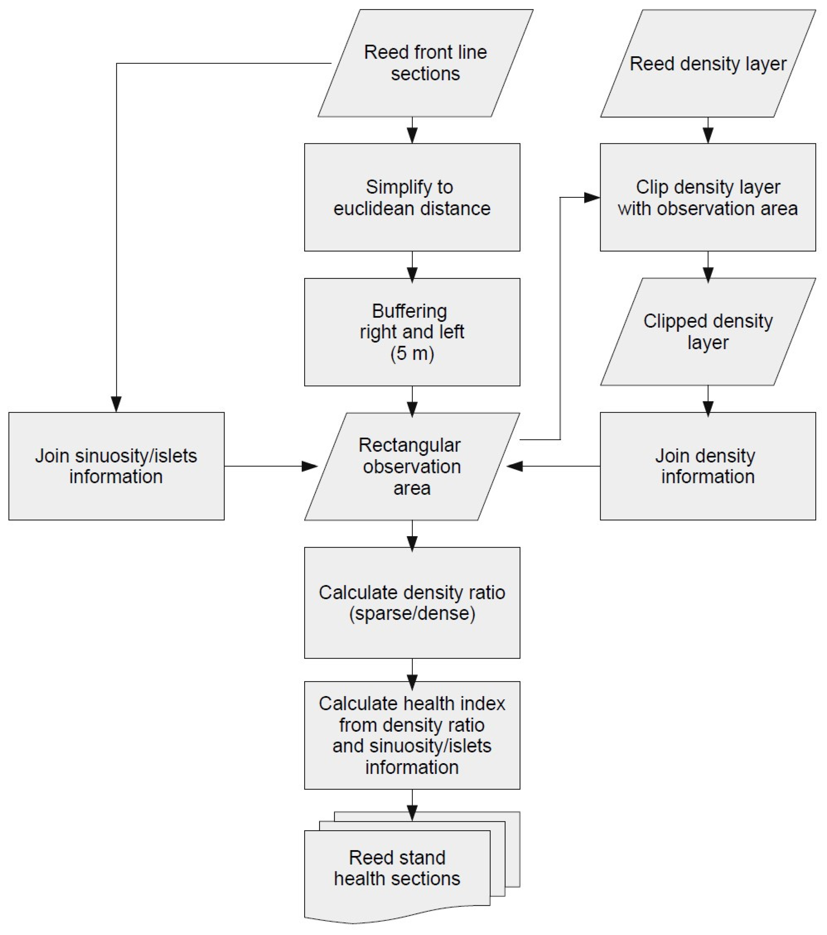
For the final aquatic reed health status estimation, we combined the above metrics, providing an “aquatic reed status index” (aRSI) following the methodological workflow as described in Figure 4.
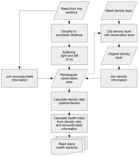
Figure 4.
Reed stand health sections flowchart.
The proposed aquatic reed status index (aRSI) is calculated as follows:
S: Sinuosity. Nislet: Number of islets per observation area. Nhole: Number of holes per observation area. Nsparse: Number of sparse reed in m2. Ndense: Number of dense reed in m2.
The aRSI results in a numerical value that can be used to assign a threshold for distinguishing stressed from healthy aquatic reed sections. This threshold has to be (can or may be) adjusted for datasets with different spatial resolutions (systems), at different sites (different lakes) and for different seasons.
2.6. Assessment of Reed Metrics Accuracies
Accuracy assessments of the previously calculated parameters ‘reed extent’, ‘reed density’ and ‘reed status’ were obtained through calculations in classical confusion matrices. As reference data, field survey data were used for ‘reed extent’ and ‘reed density’. ‘Reed status’ was visually checked against 3K RGB orthomosaics in 10 m frontline sections between the field transects for the occurrence of a frayed reed front (stressed reed), reed islets/mounds (stressed reed), and holes (stressed reed), as well as an undisturbed reed front (prospering reed) according to the definition of stressed and unstressed reed from [2]. Accuracy assessment of ‘reed height’ was checked against field-measured reed stem height data. The deviation was determined via Root Mean Square Error (RMSE).
3. Results
3.1. Aquatic Reed Heights Determination
The processing of 3K data resulted in DSM spatial resolutions between 12.8 and 13.6 cm/pix for the 14 AOIs. A visual comparison of the OHM with the orthomosaic shows plausible results. The reed front in deeper water could clearly be visually detected in the OHM.
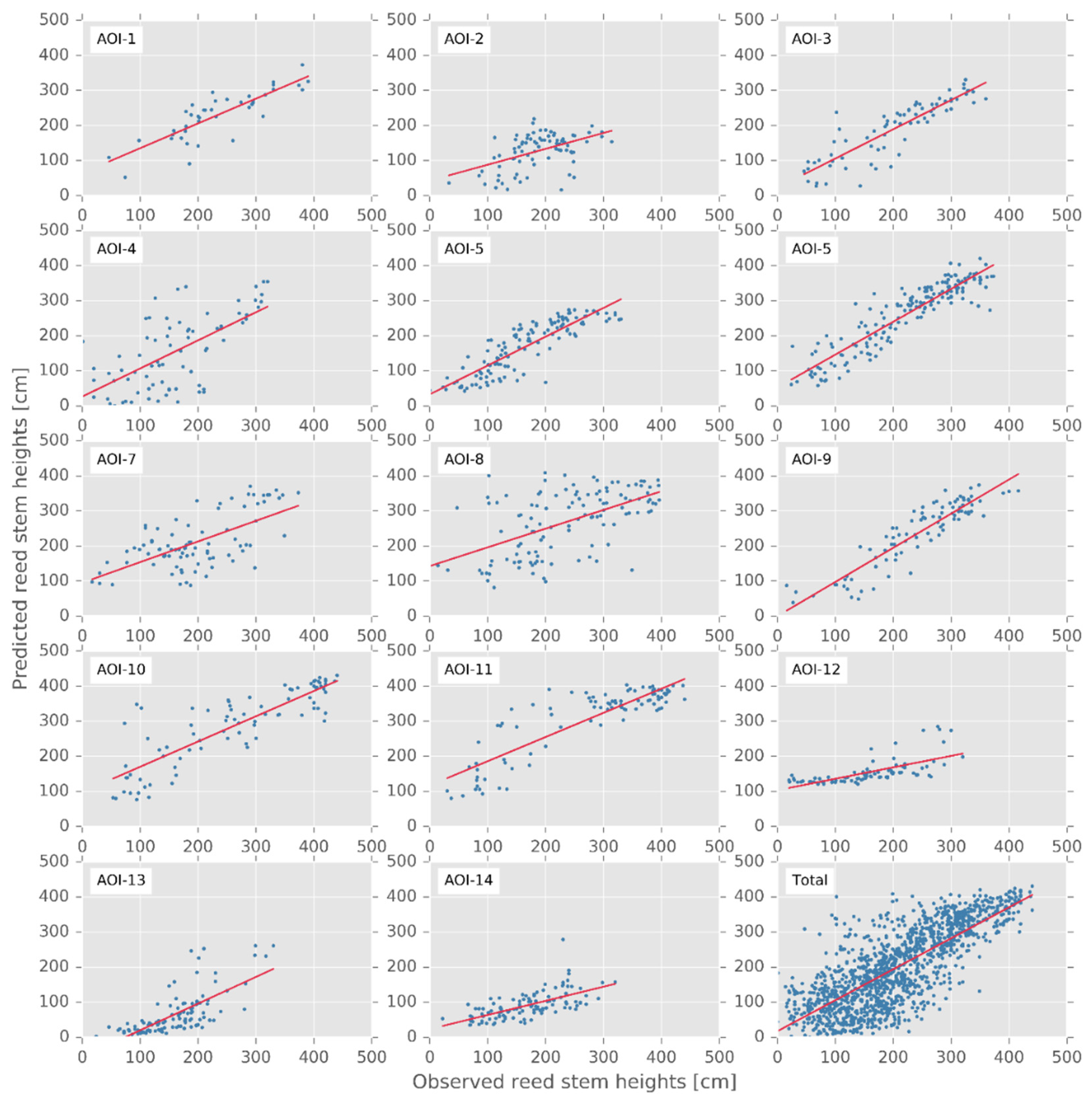
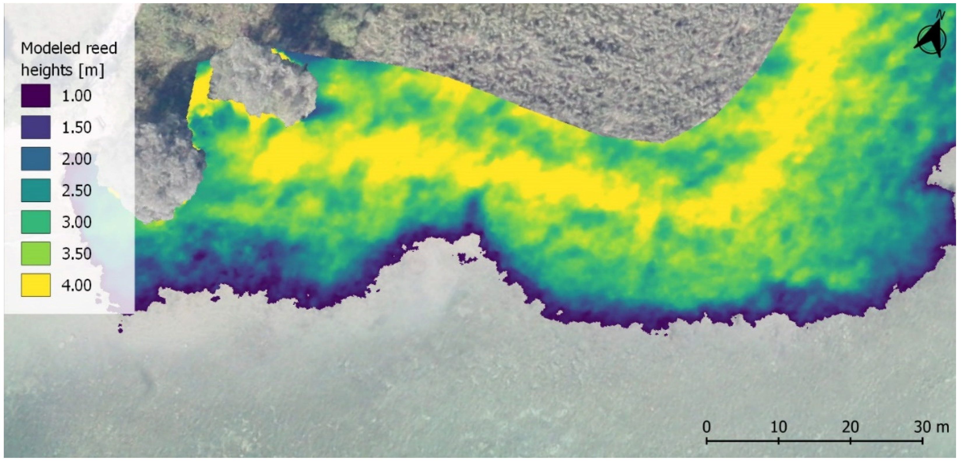
The comparison of the predicted stem heights of the aquatic reeds with the field measured heights showed a linear relationship at all AOI (Figure 5). With R2 in the range between 0.22 and 0.83 (Table 1), depending on the AOI, the goodness-of-fit of the models was variable. The total R2 with 0.60 shows an intermediate accuracy of the overall model. However, a closer look at the height estimations from 3K data and the SfM approach revealed overestimation in low-growing and slight underestimations in higher-growing reed stands. Low-growing reed stands typically occurred in deeper water and showed a lower density, while reeds in shallow water formed denser and taller stands. As illustrated in Figure 6, the highest reed stands occurred in the yellow band demarking the transition zone between aquatic and land reeds.

Figure 5.
Comparison between in situ measured reed stem heights and 3K-data-predicted stem heights for every single AOI and in total.

Table 1.
RMSE of reed stem heights at the different AOI.

Figure 6.
3K data modeled reed heights at AOI 6.
The Root Mean Square Error (RMSE) for each AOI (Table 1) shows the deviation in the vertical direction and serves as an indicator for the goodness-of-fit of the model. The total RMSE of the assessed reference points was 70 cm. In Table 1, the RMSEs for each single AOI are presented. A correlation between RMSE, R2 and the RPs horizontal DGPS precision is not clear.
3.2. Aquatic Reed Extent
The resulting reed extent geometries matched with the visual impression of the 3K RGB imagery, as well as the measured results of field campaign sections. The official landward boundary of the reed bed was always behind the end of the transects (shoreline at field data collection time) (Figure 7). We checked the accuracy of input data for the 3K modeled reed extent against our reference data measured in the field at a total of 2704 points in a confusion matrix (Table 2). The validation achieved an overall accuracy of 88% at a Kappa value of 0.77. The user accuracy (UA) indicated a classification success for aquatic reed of 91%, while the producer accuracy (PA) only reached a slightly lower value of 85%.
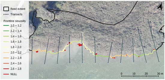
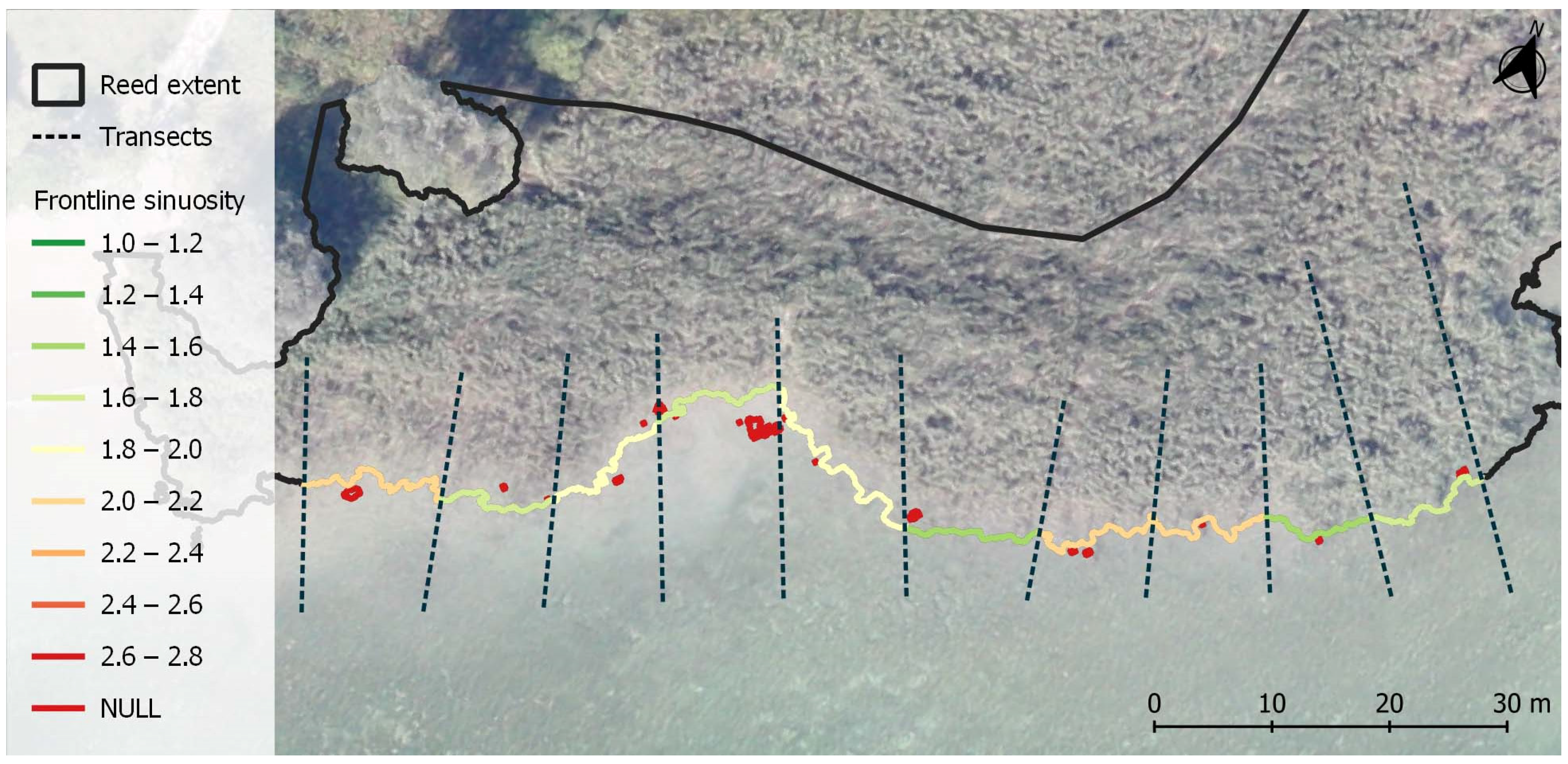
Figure 7.
Frontline sinuosity at AOI 6. NULL values represent holes in or isles within in-situ identified aquatic reed patches.
Table 2.
Accuracy assessment showing the comparison between classified reed extent areas and reference data.
3.3. Aquatic Reed Density
The aquatic reed density calculation resulted in a grid of 1 m2 raster cells representing dense and sparse reed areas (Figure 8). The classification was compared (Table 3) to the 1 m2 dense and sparse plots measured in the field, as well as open water areas on the transects. The validation of the results shows an overall accuracy of 61% and a kappa value of 0.41 (Table 3). Extremely low-density reed areas could in many cases not be detected. In general, these are single stems some meters from the frontline toward the open water. These areas are wrongly classified as water areas without reed stems. A PA of 34% for sparse reeds, in contrast to a PA of 73% for dense reeds, attests this. The result is still valuable for monitoring purposes, as the results of the UA show. For sparse and dense reeds, the UA was calculated with 71%, resp. 63%.
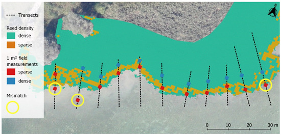
Figure 8.
Modeled aquatic reed density at AOI6 and for comparison field measurements of reed density. Mismatches between modeled and measured data are represented by yellow circles.
Table 3.
Accuracy assessment showing the comparison between classified reed densities and reference data measured in the field.
3.4. Status Estimation through Frontline Geometries
The aquatic reed front sinuosity metric is a reference variable for the disturbance of the reed front. The higher the sinuosity values, the more the aquatic reed is under pressure in the observed section (Figure 7). In addition, holes and islets were analyzed around the reed front. These are represented by all vector line parts with NULL values (closed shapes). These parts were consequently assigned to sections where the aquatic reed bed was stressed.
3.5. Aquatic Reed Status Estimation Derived by a Combinatorial Approach
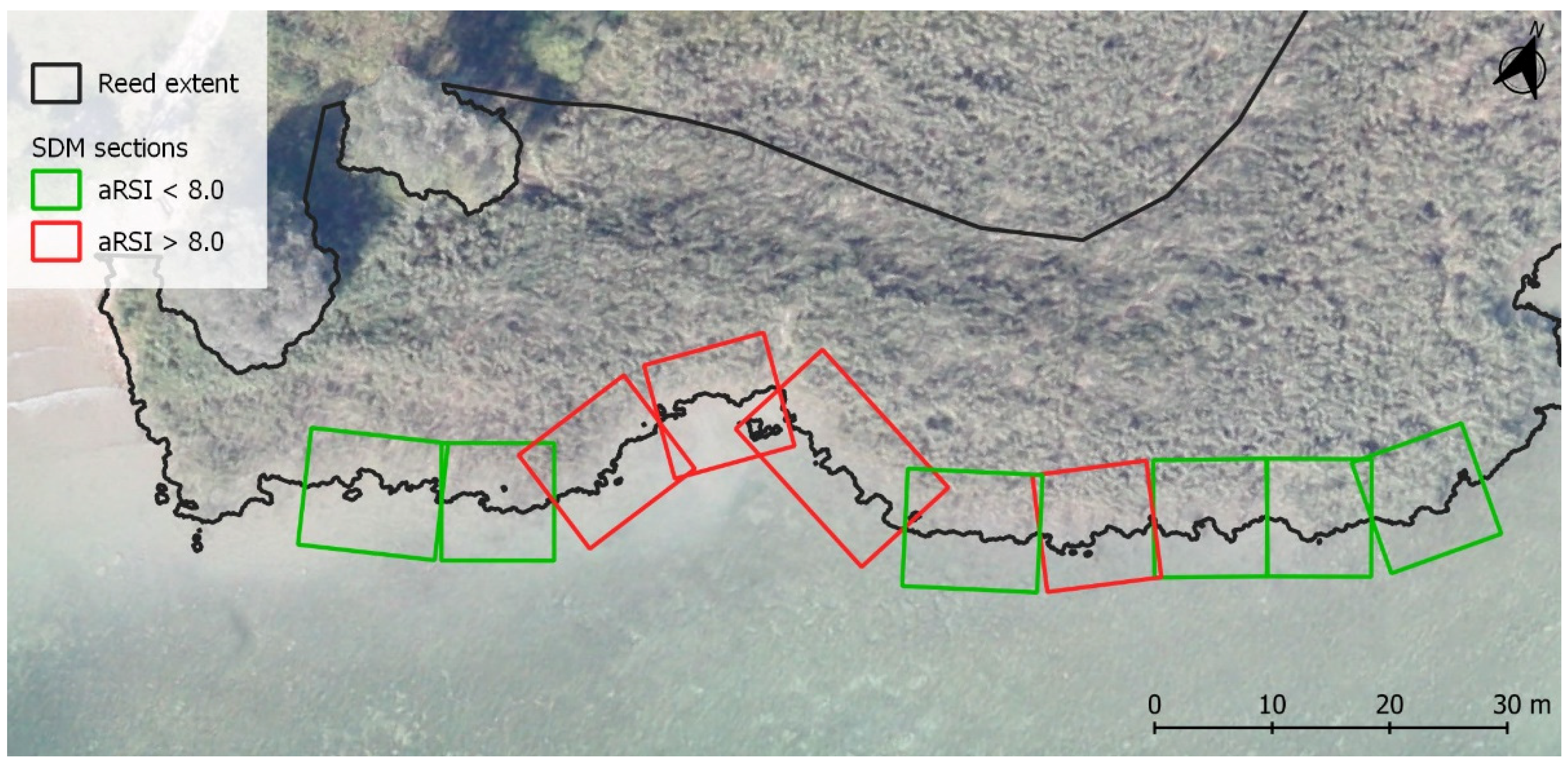
The combinatorial approach resulted in frontline sections where the aquatic reed status is either estimated as healthy or under stress. In our study site, we set the threshold as follows: Sections with aRSI values < 8.0 were classified as healthy reed areas. Sections with aRSI values > 8.0 were classified as reed areas with a critical health status (Figure 9).
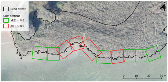
Figure 9.
Aquatic reed status estimation at AOI 6. Aquatic reeds can be assumed as under pressure in sections in red. Healthy reed sections are shown in green.
The accuracy was assessed for 117 status polygons alongside the aquatic reed front. Field transects that did not overlap with the calculated reed front because of quality issues of the DSM, were automatically excluded from the analysis. This was the case for two sections at AOI 4, seven sections at AOI 12, six sections at AOI 13 and five sections at AOI 12. The validation of the results shows an overall accuracy of 81.20% and a kappa value of 0.61, which can be interpreted as substantial (Table 4). The accuracy assessment also shows that the aRSI is less sensitive for stressed reeds (PA 0.67%) than for healthy reed sections (PA 0.92%).
Table 4.
Accuracy matrix for the status estimation derived by a combinatorial approach.
4. Discussion
With regard to the expected support of aquatic reed monitoring by remote sensing methods, we analyzed the capability of the photogrammetric 3K camera system, developed and operated by DLR. The results of this study suggest that SfM digital surface model generation from data collected by the 3K airborne multi-camera system is accurate enough to provide the basic information needed to estimate the aquatic reed status of freshwater lakes. This is still valid, even if slight over- or underestimations of reed heights as the base parameter, derived reed extents and reed densities cannot be fully avoided.
4.1. Aquatic Reed Heights
The critical variable of our approach was the aquatic reed height. Proper modeling of reed heights was the most important step in our processing chain. All following parameters (extent, front line, density, reed status) we derived from the heights. Therefore, the quality of the following variables is directly controlled by the quality of the photogrammetric SfM process.
The validation process of the 3K data analysis results in an overall RMSE of 70 cm, with RMSE for individual AOI ranging between 39 cm and 104 cm.
These results are slightly inferior, but still comparable to studies of SfM approaches with UAV data of agricultural crop stands [25,26]. Wachholz De Souza et al. [26] achieved RMSEs between 40 cm and 57 cm for height estimations for sugar cane studies, Geipel et al. [25] working over corn with IMU-based georeferenced drone UAV data reported RMSEs between 27 cm and 38 cm for their height calculations. In the case of agricultural crop stands there are no attenuations by the waterbody (wind, refraction, multiple scattering, mirror-like reflection, wave focusing effects, etc.), as is the case with aquatic reed stands. Under conditions comparable to our 3K data study, the results from camera systems mounted on fixed-wing and copter UAVs, as reported by Corti et al. (2018) from the same study site at Lake Chiemsee, showed considerably lower accuracies, with RMSEs of 104 cm and 142 cm, respectively [28].
The more precise estimation of the height parameter by the 3K data analysis was mainly explained by the much more stable flight path of the airplane and the precise IMU data supporting the 3K data, in contrast to the UAV without an IMU. In addition, it could be that the 3K system observes the object “reed” from different angles, and thus more information is available in the data set for DSM modeling. Moreover, the airborne 3K System used in this study, mounted on an airplane and used for imaging from 1000 a.g.l., has further advantages over drone systems, such as faster image acquisition times and larger coverages of investigation areas. In case of the abovementioned UAV study by Corti et al. (2018), it was not possible to image all AOIs within one day, especially not under comparable illumination condition.
Regarding the apparently high RMSE for some AOIs, it must be considered that aquatic reed stands are object types that continuously (phenology) or spontaneously (wind, wave, induced movements of the canopy, mechanical disturbances) change their appearances. In addition, AOIs are exposed to different wind/wave expositions.
A general, valid source of errors is the period of up to 20 days between field measurements and the remote sensing overflight. Field campaigns are time-consuming and weather-dependent. Therefore, to cover such large areas, it is practically impossible to schedule the flight day and the field campaign on the same day. Heavy winds and waves often occur in September at Lake Chiemsee and could have overturned larger areas of reed stems before the date of the flight campaign.
Another explanation, e.g., for AOI 13 (RMSE 104 cm) and AOI 14 (RMSE 90 cm), is the permanent influence of heavy waves resulting from crossing passenger ferries.
Moreover, estimation errors for sparse reed stands could be explained through the adverse effects of the water surface between the single reed stems. Due to different image acquisition positions and water movements, reflection effects and ripples differ from image to image. SfM algorithms have difficulties in the image alignment process, either not finding proper pixels or misinterpreting the position of pixels suitable for tie points [39]. All of these factors may sum up to the observed higher disturbances, and thus higher residual values especially for sparse reed stands.
Under such circumstances, the RMSE, although still being high, seems nevertheless acceptable. The determination of reed extent and reed density on the basis of heights seem reasonable.
4.2. Reed Extent
Regarding aquatic reed extent areas, it must be mentioned that, between aquatic and land reeds, there is a changing zone of transition reeds controlled by the water level at the time of observation. This situation was well displayed when comparing the land side ends of the transects for in-situ data sampling and the ‘official’ shore line. Water level during the sampling period and 3K data collection was 517.96 m a.s.l. lower than the mean water level of the last ten years which was measured with 518.20 m a.s.l.
In our study, aquatic reed extent was determined through the reed heights. This causes the previously mentioned problems in the height model to be dragged further towards the precision of the classification of the areal extent. Especially at AOI 12, AOI 13 and AOI 14, the quality of the DSM was lower. These areas are located on the western shore of the island, Herrenchiemsee; therefore, as described above, these areas are under the heavy influence of waves from ferries, as well as from prevailing westerly winds. This means that wave-affected water surfaces resulting in multiple reflections superimposing the reed signal, as well as the wind-caused movements of the canopy changing the geometry of the surface between the single data takes, are some of the reasons that explain the high RMSE values calculated.
The accuracy assessment, especially the low PA for low-density aquatic reed areas, indicates that the proportion of aquatic reed that was not detected is far greater than the proportion of water areas incorrectly classified as areas with reed. We suspect that the spatial resolution of the sensor technology is the main limiting factor. At pixel sizes of 0.14 m, the sensor seems unable to resolve individual reed stems. On the other hand, Corti et al. analyzed data of much higher spatial resolutions (0.02 to 0.05 m) recorded from UAVs and found similar RMSE ranges for low-density aquatic reeds. This indicates that the most probable reason for these results is water surface effects such as sun glint, in combination with neighborhood effects from the brighter lake bottom in shallow areas, which superimpose the reflected signal of reed stems. Regardless, with 88% overall accuracy, the results show a high correctness for classifying the extent of aquatic reeds at Lake Chiemsee.
4.3. Aquatic Reed Density
The approach of classifying reed density by height and variance was also found to be accurate enough to deduce information on reed stand condition. When classifying the reed density, very loose water reeds were partly not identified. There are several reasons for this, which could also have been present in combination. It is possible that the spatial resolution from the 3K system was not sufficient. Another reason could be adjustment errors in the photogrammetric process chain. The 3K system provides a classification with an overall accuracy of over 60% and a kappa value of 0.41. These values have to be interpreted as moderate results. It must be noted that these are local-scale analyses in the range of less than one meter. Producer, user and overall accuracy prove that the 3K system and the applied methodology are well-suited for determining aquatic reed densities. Integrated in a multi-parameter decision chain, as proposed by this study, the density variable can be helpful for estimating the status of aquatic reed growing in freshwater lakes.
4.4. Status Estimation through Frontline Geometries
Within the traditional reed surveys reed frontline status is one, if not the most important diagnostic feature. One reason is the accessibility from the lakeside by boat. The sinuosity proved to be a variable with a high explanatory power for analyzing the status of the reed front [23]. For the status estimation of the frontline geometries, the methodology of Corti et al. [23] was modified by automatically classifying holes in the aquatic reed beds and islets of reed in the open water. Our study demonstrated that, especially the last two parameters, contributed valuable information for depicting damaged reed sections [13]. In our approach, sinuosity plays an important role as an integral part of the aquatic reed status index (aRSI).
4.5. Aquatic Reed Status Estimation Derived by a Combinatorial Approach
A combinatorial approach is highly dependent on the preceding processing steps. The modeling of reed height is especially critical because all other variables that are combined to the aRSI, such as aquatic reed area and density, are derived from reed heights. In our study, 20 out of 137 possible reed sections could not be evaluated by our automatic processing chain. Nevertheless, the validation of the 107 remaining aquatic reed sections demonstrated that the aRSI provides accurate assessments of the status of aquatic reed bed sections, wherever the processing is successful. However, it can be expected that the thresholds generating the best results in our study must be adjusted for data sets with different spatial resolutions.
The implications of this assessment for aquatic and coastal landscape management include the provision of a less time-consuming monitoring tool that can facilitate decision making, e.g., by the accurate identification of areas under stress or undergoing fast deterioration. Moreover, the “human factor” of a qualitative assessment clearly has its weak points when it comes to transferring results. Here, the automatic processing with its quantitative results can be more suited as a transferable basis for decision making.
5. Conclusions
The airborne photogrammetric 3K system, in combination with an SfM-based approach, proves practicability in depicting and analyzing wetlands and in the specific case of estimating aquatic reed heights. The 3K system thus qualified as an independent system for the monitoring of water reed stands, offering high-spatial-resolution data suitable as a basis for the further fully automated analysis of reed beds. The system provides RGB data from which orthomosaics can be produced, precisely locating the reed stands and deriving their status. The strengths of the 3K system can clearly be seen in the structural analysis, which can be carried out from the three-dimensional structural data provided by the structure-from-motion method. Despite the presented advantages, the aspect of a varying accuracy ranging from 60–90% needs to be considered. Poorer accuracies mainly relate to reed density analyses, where the resolution of the sensor and optics play a greater role in the detection of narrow objects, such as reed stems. We are sure that the results could be further improved with higher-resolution sensor systems and refined SfM algorithms.
Next, regarding the estimation of aquatic reed heights, the dataset shows further benefits. Aside from the areas covered with Phragmites australis, neighboring vegetation such as trees, and anthropogenic structures such as jetties and boat houses, were properly modeled. This information may be useful for further studies of the lake–shore structure.
Overall, the developed processing approach can be seen as an advantageous methodological alternative for monitoring aquatic reed beds in contrast to classical approaches such as field surveys or the visual interpretation of aerial images.
Author Contributions
The project idea was conceived by T.S. and S.B. processed the image collections, analyzed the data, and drafted the manuscript. N.C.M. contributed to the experimental design, measurement campaign, and as well as, J.G. and T.S. to conceptualizing, writing and editing of the manuscript. All authors have read and agreed to the published version of the manuscript.
Funding
This research was funded by the Bavarian State Ministry of the Environment and Consumer Protection (grant number TLK01U-66627). The APC was funded by the Chair of Aquatic Systems Biology of the Technical University of Munich.
Informed Consent Statement
Not applicable.
Data Availability Statement
Not applicable.
Acknowledgments
Conducted in the scope of the project “Bayerns Stillgewässer im Klimawandel—Einfluss und Anpassung” (TLK01U-66627), this study is a partial project “Klimawandel beeinträchtigt Schilfbestände bayerischer Seen—Erfassung mittels moderner Monitoringmethoden” sponsored by the Bavarian State Ministry of the Environment and Consumer Protection. We thank this organization for contributing to the research on monitoring aquatic reed beds in the Bavarian lakes. Our special thanks go to Tanja Gschlössl, who accompanied our study with great interest and helpful suggestions across the whole duration of the project. In addition, we would like to thank Tatjana Bodmer, Dana Lippert, and Manuel Güntner for their contribution in the fieldwork.
Conflicts of Interest
The authors declare no conflict of interest.
References
- Gigante, D.; Venanzoni, R.; Zuccarello, V. Reed Die-Back in Southern Europe? A Case Study from Central Italy. Comptes Rendus Biol. 2011, 334, 327–336. [Google Scholar] [CrossRef]
- Grosser, S.; Melzer, A.; Pohl, W. Untersuchung des Schilfrückgangs an Bayerischen Seen: Forschungsprojekt des Bayerischen Staatsministeriums für Landesentwicklung und Umweltfragen; Bayerisches Landesamt für Umweltschutz: Wielenbach, Germany, 1997. [Google Scholar]
- Krumscheid, P.; Stark, H.; Peintinger, M. Decline of Reed at Lake Constance (Obersee) Since 1967 Based on Interpretations of Aerial Photographs. Aquat. Bot. 1989, 35, 57–62. [Google Scholar] [CrossRef]
- Ostendorp, W. “Die-Back” of Reeds in Europe: A Critical Review of Literature. Aquat. Bot. 1989, 35, 5–26. [Google Scholar] [CrossRef] [Green Version]
- Rücker, A.; Grosser, S.; Melzer, A. Geschichte und Ursachen des Röhrichtrückgangs Am Ammersee (Deutschland). Limnol.—Ecol. Manag. Inland Waters 1999, 29, 11–20. [Google Scholar] [CrossRef] [Green Version]
- van der Putten, W.H. Die-Back of Phragmites Australis in European Wetlands: An Overview of the European Research Programme on Reed Die-Back and Progression (1993–1994). Aquat. Bot. 1997, 59, 263–275. [Google Scholar] [CrossRef]
- Ostendorp, W.; Dienst, M.; Schmieder, K. Disturbance and Rehabilitation of Lakeside Phragmites Reeds Following an Extreme Flood in Lake Constance (Germany). Hydrobiologia 2003, 506–509, 687–695. [Google Scholar] [CrossRef] [Green Version]
- Schmieder, K.; Dienst, M.; Ostendorp, W.; Jöhnk, K.D. Effects of Water Level Variations on the Dynamics of the Reed Belts of Lake Constance. Int. J. Ecohydrol. Hydrobiol. 2004, 4, 469–480. [Google Scholar]
- Melzer, A.; Harlacher, R.; Held, K.; Sirch, R.; Vogt, E. Die Makrophytenvegetation des Chiemsees; Bayerisches Landesamt für Wasserwirtschaft: Munich, Germany, 1986. [Google Scholar]
- Sukopp, H. Conservation of Wetlands in Central Europe. Available online: https://eurekamag.com/research/026/316/026316883.php (accessed on 17 May 2017).
- Dienst, M.; Schmieder, K.; Ostendorp, W. Dynamik der Schilfröhrichte am Bodensee unter dem Einfluss von Wasserstandsvariationen. Eff. Water Level Var. Dyn. Reed Belts Lake Constance 2004, 34, 29–36. [Google Scholar] [CrossRef] [Green Version]
- LfU, Referat 51 Kartieranleitung Biotopkartierung Bayern (Inkl. Kartierung Der Offenland-Lebensraumtypen Der Fauna-Flora-Habitat-Richtlinie)—Teil 1—Arbeitsmethodik 2018. Available online: https://www.lfu.bayern.de/natur/doc/kartieranleitungen/arbeitsmethodik_teil1.pdf (accessed on 10 January 2022).
- Hoffmann, F.; Zimmermann, S. Chiemsee Schilfkataster. 1973, 1979, 1991 und 1998; Limnologische Station der Technischen Universität München: Iffeldorf, Germany, 2000. [Google Scholar]
- Rosso, P.H.; Ustin, S.L.; Hastings, A. Mapping Marshland Vegetation of San Francisco Bay, California, Using Hyperspectral Data. Int. J. Remote Sens. 2005, 26, 5169–5191. [Google Scholar] [CrossRef]
- Andresen, T.; Mott, C.; Zimmermann, S.; Schneider, T.; Melzer, A. Object-Oriented Information Extraction for the Monitoring of Sensitive Aquatic Environments. In Proceedings of the IEEE International Geoscience and Remote Sensing Symposium, Toronto, ON, Canada, 24–28 June 2002; IEEE: Piscataway, NJ, USA, 2002; Volume 5, pp. 3083–3085. [Google Scholar]
- Villa, P.; Laini, A.; Bresciani, M.; Bolpagni, R. A Remote Sensing Approach to Monitor the Conservation Status of Lacustrine Phragmites Australis Beds. Wetl. Ecol. Manag. 2013, 21, 399–416. [Google Scholar] [CrossRef]
- Villa, P.; Bresciani, M.; Braga, F.; Bolpagni, R. Comparative Assessment of Broadband Vegetation Indices Over Aquatic Vegetation. IEEE J. Sel. Top. Appl. Earth Obs. Remote Sens. 2014, 7, 3117–3127. [Google Scholar] [CrossRef]
- Villa, P.; Bresciani, M.; Bolpagni, R.; Pinardi, M.; Giardino, C. A Rule-Based Approach for Mapping Macrophyte Communities Using Multi-Temporal Aquatic Vegetation Indices. Remote Sens. Environ. 2015, 171, 218–233. [Google Scholar] [CrossRef] [Green Version]
- Gilmore, M.S.; Wilson, E.H.; Barrett, N.; Civco, D.L.; Prisloe, S.; Hurd, J.D.; Chadwick, C. Integrating Multi-Temporal Spectral and Structural Information to Map Wetland Vegetation in a Lower Connecticut River Tidal Marsh. Remote Sens. Environ. 2008, 112, 4048–4060. [Google Scholar] [CrossRef]
- Samiappan, S.; Turnage, G.; Hathcock, L.A.; Moorhead, R. Mapping of Invasive Phragmites (Common Reed) in Gulf of Mexico Coastal Wetlands Using Multispectral Imagery and Small Unmanned Aerial Systems. Int. J. Remote Sens. 2017, 38, 2861–2882. [Google Scholar] [CrossRef]
- Zlinszky, A.; Mücke, W.; Lehner, H.; Briese, C.; Pfeifer, N. Categorizing Wetland Vegetation by Airborne Laser Scanning on Lake Balaton and Kis-Balaton, Hungary. Remote Sens. 2012, 4, 1617–1650. [Google Scholar] [CrossRef] [Green Version]
- Iglhaut, J.; Cabo, C.; Puliti, S.; Piermattei, L.; O’Connor, J.; Rosette, J. Structure from Motion Photogrammetry in Forestry: A Review. Curr. For. Rep. 2019, 5, 155–168. [Google Scholar] [CrossRef] [Green Version]
- Corti Meneses, N.; Brunner, F.; Baier, S.; Geist, J.; Schneider, T. Quantification of Extent, Density, and Status of Aquatic Reed Beds Using Point Clouds Derived from UAV–RGB Imagery. Remote Sens. 2018, 10, 1869. [Google Scholar] [CrossRef] [Green Version]
- Bendig, J.; Bolten, A.; Bareth, G. UAV-Based Imaging for Multi-Temporal, Very High Resolution Crop Surface Models to Monitor Crop Growth VariabilityMonitoring des Pflanzenwachstums Mit Hilfe Multitemporaler und Hoch Auflösender Oberflächenmodelle von Getreidebeständen Auf Basis von Bildern Aus UAV-Befliegungen. Photogramm. Fernerkund. Geoinf. 2013, 2013, 551–562. [Google Scholar] [CrossRef]
- Geipel, J.; Link, J.; Claupein, W. Combined Spectral and Spatial Modeling of Corn Yield Based on Aerial Images and Crop Surface Models Acquired with an Unmanned Aircraft System. Remote Sens. 2014, 6, 10335–10355. [Google Scholar] [CrossRef] [Green Version]
- Wachholz De Souza, C.H.; Camargo Lamparelli, R.A.; Rocha, J.V.; Graziano Magalhães, P.S. Height Estimation of Sugarcane Using an Unmanned Aerial System (UAS) Based on Structure from Motion (SfM) Point Clouds. Int. J. Remote Sens. 2017, 38, 2218–2230. [Google Scholar] [CrossRef]
- Corti Meneses, N.; Baier, S.; Geist, J.; Schneider, T. Evaluation of Green-LiDAR Data for Mapping Extent, Density and Height of Aquatic Reed Beds at Lake Chiemsee, Bavaria—Germany. Remote Sens. 2017, 9, 1308. [Google Scholar] [CrossRef] [Green Version]
- Corti Meneses, N.; Baier, S.; Reidelstürz, P.; Geist, J.; Schneider, T. Modelling Heights of Sparse Aquatic Reed (Phragmites Australis) Using Structure from Motion Point Clouds Derived from Rotary- and Fixed-Wing Unmanned Aerial Vehicle (UAV) Data. Limnologica 2018, 72, 10–21. [Google Scholar] [CrossRef]
- Koma, Z.; Zlinszky, A.; Bekő, L.; Burai, P.; Seijmonsbergen, A.C.; Kissling, W.D. Quantifying 3D Vegetation Structure in Wetlands Using Differently Measured Airborne Laser Scanning Data. Ecol. Indic. 2021, 127, 107752. [Google Scholar] [CrossRef]
- Reinartz, P.; Kurz, F.; Rosenbaum, D.; Leitloff, J.; Palubinskas, G. Image Time Series for Near Real Time Airborne Monitoring of Disaster Situations and Traffic Applications. In Modeling of Optical Airborne and Space Borne Sensors; Copernicus Gesellschaft Mbh: Gottingen, Germany, 2010; Volume 38-1. [Google Scholar]
- Roemer, H.; Kiefl, R.; Henkel, F.; Wenxi, C.; Nippold, R.; Kurz, F.; Kippnich, U. Using Airborne Remote Sensing to Increase Situational Awareness in Civil Protection and Humanitarian Relief—The Importance of User Involvement. In Xxiii Isprs Congress, Commission Viii; Halounova, L., Safar, V., Raju, P.L.N., Planka, L., Zdimal, V., Kumar, T.S., Faruque, F.S., Kerr, Y., Ramasamy, S.M., Comiso, J., et al., Eds.; Copernicus Gesellschaft Mbh: Goettingen, Germany, 2016; Volume 41, pp. 1363–1370. [Google Scholar]
- Thomas, U.; Rosenbaum, D.; Kurz, F.; Suri, S.; Reinartz, P. A New Software/Hardware Architecture for Real Time Image Processing of Wide Area Airborne Camera Images. J. Real-Time Image Proc. 2009, 4, 229. [Google Scholar] [CrossRef]
- Kurz, F. Accuracy Assessment of the DLR 3K Camera System. In Proceedings of the DGPF Tagungsband; Seyfert, E., Ed.; Deutsche Gesellschaft für Photogrammetrie, Fernerkundung und Geoinformation: Jena, Germany, 2009; Volume 18, pp. 1–7. [Google Scholar]
- LfU Bayern Seen in Bayern—LfU Bayern. Available online: https://www.lfu.bayern.de/wasser/seen_in_bayern/index.htm (accessed on 23 May 2017).
- Brocks, S.; Bendig, J.; Bareth, G. Toward an Automated Low-Cost Three-Dimensional Crop Surface Monitoring System Using Oblique Stereo Imagery from Consumer-Grade Smart Cameras. J. Appl. Remote Sens. 2016, 10, 046021. [Google Scholar] [CrossRef] [Green Version]
- Jensen, J.L.R.; Mathews, A.J. Assessment of Image-Based Point Cloud Products to Generate a Bare Earth Surface and Estimate Canopy Heights in a Woodland Ecosystem. Remote Sens. 2016, 8, 50. [Google Scholar] [CrossRef] [Green Version]
- Weiss, M.; Baret, F. Using 3D Point Clouds Derived from UAV RGB Imagery to Describe Vineyard 3D Macro-Structure. Remote Sens. 2017, 9, 111. [Google Scholar] [CrossRef] [Green Version]
- QGIS Development Team. QGIS Geographic Information System. Open Source Geospatial Foundation Project; QGIS Development Team: Chur, Switzerland, 2020. [Google Scholar]
- Kerner, S.; Kaufman, I.; Raizman, Y. Role of Tie-Points Distribution in Aerial Photography. In Eurocow 2016, the European Calibration and Orientation Workshop; Skaloud, J., Colomina, I., Eds.; Copernicus Gesellschaft Mbh: Gottingen, Germany, 2016; Volumes 40–43, pp. 41–44. [Google Scholar]

Publisher’s Note: MDPI stays neutral with regard to jurisdictional claims in published maps and institutional affiliations. |
© 2022 by the authors. Licensee MDPI, Basel, Switzerland. This article is an open access article distributed under the terms and conditions of the Creative Commons Attribution (CC BY) license (https://creativecommons.org/licenses/by/4.0/).