Abstract
Using a multiple-input-multiple-output (MIMO) radar for environment sensing is gaining more attention in unmanned ground vehicles (UGV). During the movement of the UGV, the position of MIMO array compared to the ideal imaging position will inevitably change. Although compressed sensing (CS) imaging can provide high resolution imaging results and reduce the complexity of the system, the inaccurate MIMO array elements position will lead to defocusing of imaging. In this paper, a method is proposed to realize MIMO array motion error compensation and sparse imaging simultaneously. It utilizes a block coordinate descent (BCD) method, which iteratively estimates the motion errors of the transmitting and receiving elements, as well as synchronously achieving the autofocus imaging. The method accurately estimates and compensates for the motion errors of the transmitters and receivers, rather than approximating them as phase errors in the data. The validity of the proposed method is verified by simulation and measured experiments in a smoky environment.
1. Introduction
The application of unmanned ground vehicles allows the performance of operations in areas inaccessible to humans due to chemical, biological, thermal, and other environmental hazards [1]. The MIMO radar becomes an alternative to the full array when only a small number of array elements is used to meet the demands for high azimuth and elevation resolution [2]. For an antenna of a predetermined size, MIMO array is often applied to accomplish rapid imaging and cut down the number of array elements in order to economize on the hardware cost [3,4,5,6,7]. Therefore, advanced UGVs are equipped with various types of MIMO radar [8].
In [9], through increasing the variety of radiation, a method called radar coincidence imaging is studied. Time-reversal imaging is applied to MIMO radar imaging problems [10,11,12]. In [13], an imaging method combining the range migration and the back projection (BP) is proposed for arbitrary scanning paths. However, the azimuth resolution is restricted to the length of the received array. In [14,15], different spectral estimation algorithms are used to enhance azimuth resolution and to compress sidelobes. The theory of compressed sensing (CS) [16] provides the possibility of solving the underdetermined problem. In [17], a segmented random sparse method based on CS is presented to ensure the accuracy of 3-D reconstruction. CS has been introduced to the radar-related applications, such as ground-penetrating radar [18], through-the-wall imaging [19], and inverse SAR (ISAR) [20].
A basic difficulty in MIMO radar imaging is imperfect knowledge of the real position of the array. Providing real-time and accurate vehicle posture information is one of the key technologies to achieve conditional and even highly autonomous driving [21]. During the movement of UGV, unknown road information, such as the road inclination angle, tire-road friction coefficient, and road slope angle [22], will lead to motion errors of the MIMO array. In the real environment, the inertial measurement units (INS) or Global Positioning System (GPS) circuits, generally provide reasonably accurate but inaccurate locations. The unsolved uncertainty can be solved by data-driven autofocus algorithms [23,24,25].
Extensive literature settles the radar autofocus problem by estimating a substituted collection of phase errors in the measured signal, instead of the position errors [26,27,28,29,30]. In [31], an autofocus method is proposed for compressively sampled SAR. In [32,33], autofocusing technology is proposed to correct the phase errors. In [34], a CS imaging with compensation of the observation position error method is proposed to reconstruct the image and correct the errors in the SAR structure. A joint sparsity-based imaging and motion error estimation algorithm is utilized to obtain focused images [35]. A blind deconvolution method is proposed to acquire autofocus images from observations that undergo a position error [36]. However, it can only solve the problem when antennas are influenced by the identical position error. Table 1 shows the categories of methods used to solve autofocus problems.

Table 1.
Categories of methods to solve autofocus problems.
We propose a method to compensate for the motion errors of the MIMO radar array in CS imaging. It is modeled as an optimization problem in which the cost function includes the motion errors of transmitters and receivers and the reflectivity coefficients of targets. The main contributions are as follows:
- (1)
- We analyzed the essential relationship between the motion errors of array and CS imaging. The proposed method takes effect on estimating the MIMO array motion errors as well as reconstructing images, which is without any approximations.
- (2)
- The optimization problem is solved by a BCD method, which cycles through steps of target reconstruction and MIMO array motion errors estimation and compensation. The motion errors of transmitters and receivers can be estimated by gradient-based optimization algorithms.
- (3)
- Based on the accurate estimation of the motion errors, we can achieve super-resolution imaging. Compared with optical sensors, in special circumstances, such as smoke scenes, it has a better environmental perception ability.
This paper consists of 5 parts. In Section 2, the method proposed in this paper is introduced, i.e., the geometry model and signal model for MIMO radar imaging are described in Section 2.1 and CS imaging with motion errors compensation and computational complexity are depicted in Section 2.2. In Section 3, simulation and experiment results are presented. Section 4 provides the discussion. Section 5 will summarize this paper.
Throughout the text, lower case bold face letters denote vectors and upper case bold face letters denote matrices. Superscripts and refer to the transpose of matrices and the Hermitian of matrices. The norm of a vector is defined as the sum of its absolute values, i.e., . The norm of a vector is defined as the square root of the sum of its squares, i.e., .
2. Materials and Methods
2.1. MIMO Radar Imaging Model
2.1.1. Geometry Model
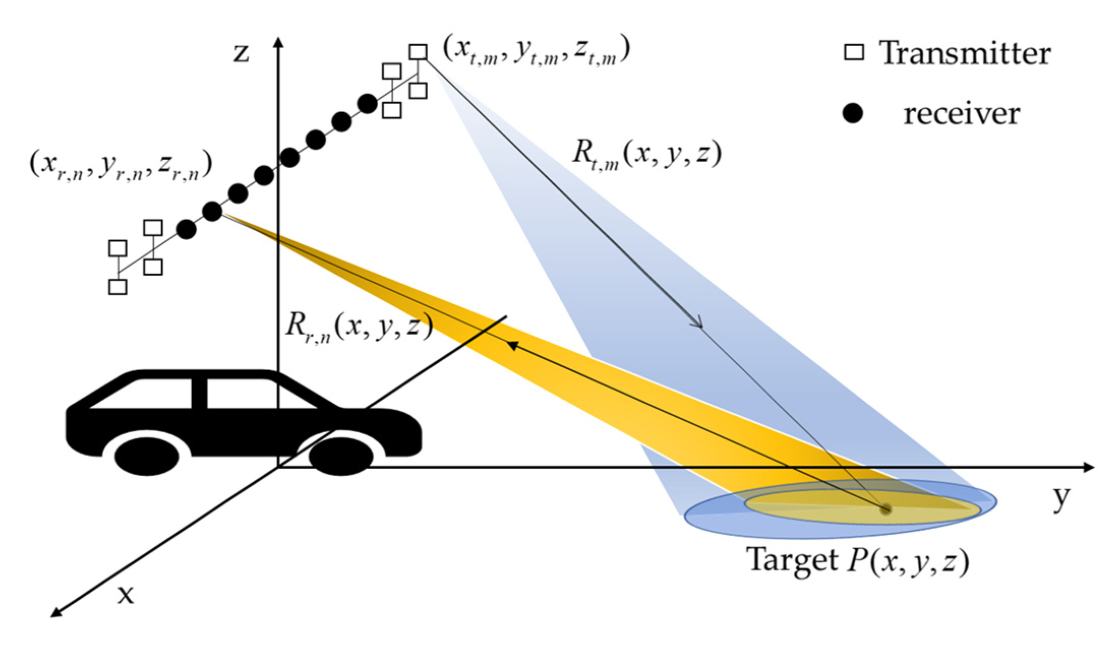
Consider a MIMO array that has transmitters and receivers. Figure 1 illustrates the MIMO array mounted on UGV, is azimuth direction and where is the forward direction. Supposing the position vector of transmitting element is and the position vector of receiving element is , where , , , , , are coordinates in the Cartesian coordinate system. The real time position vectors of transmitting element and receiving element are denoted as and , respectively,
where and depict the real motion error vector of the transmitting element and receiving element, respectively. We set the position vectors of the target to be , the instantaneous two-way range of target of the transmitting element and the receiving element can be expressed as
where and denote the instantaneous real range from the transmitting element to target and target to the receiving element, respectively,

Figure 1.
Imaging geometry of MIMO Radar.
The hypothetical two-way range for target without any motion errors are expressed as
where and denote the ideal range from the transmitting element to target and target to the receiving element, respectively,
2.1.2. Signal Model
Assume that the stepped frequency is transmitted by the MIMO radar and the data of the receiving element from the transmitting element can be expressed as
where and are the coordinates of the target and is the reflectivity coefficient of the target at ; is the two-way range of the target at of the transmitter and the receiver; is the value of frequency; depicts the speed of light; is the area illuminated by the beam.
Based on (8), the discrete expression of the echo of the receiving element from the transmitting element is
where the is the total number of grid points after the discretization of the scene, is the reflectivity coefficient of the point, and is the two-way range of point of the transmitter and the receiver. The equation for is shown in (2).
Equation (9) can be expressed in matrix form as
where is a signal vector, is a measurement matrix, and is a target vector. is the total number of frequencies, is the total number of receivers, is the total number of transmitters. The vector/matrix terms in (10) are depicted by the following equations, where
2.2. CS Imaging with Motion Errors Compensation
In this section, CS Imaging is achieved by estimating the radar cross section (RCS) information and motion errors. As depicted in (10), is the received signal. is the measurement matrix. Owing to the MIMO array, the position cannot be acquired precisely, often involves errors, which have an impact on the reconstruction of targets .
As a consequence, knowing the inaccuracy position of the MIMO array and denoting the as a function in connection with errors, i.e., , where and denote the transmitters motion errors and the receivers motion errors, respectively,
The model in (10) can be modified to
Considering the array motion errors, except for the imaging, we should achieve the estimation of the array motion errors. We express the process of imaging and estimating the array motion errors as the minimization of the cost function below
where is the regularization parameter, which balances the imaging fidelity and the sparsity of the solution.
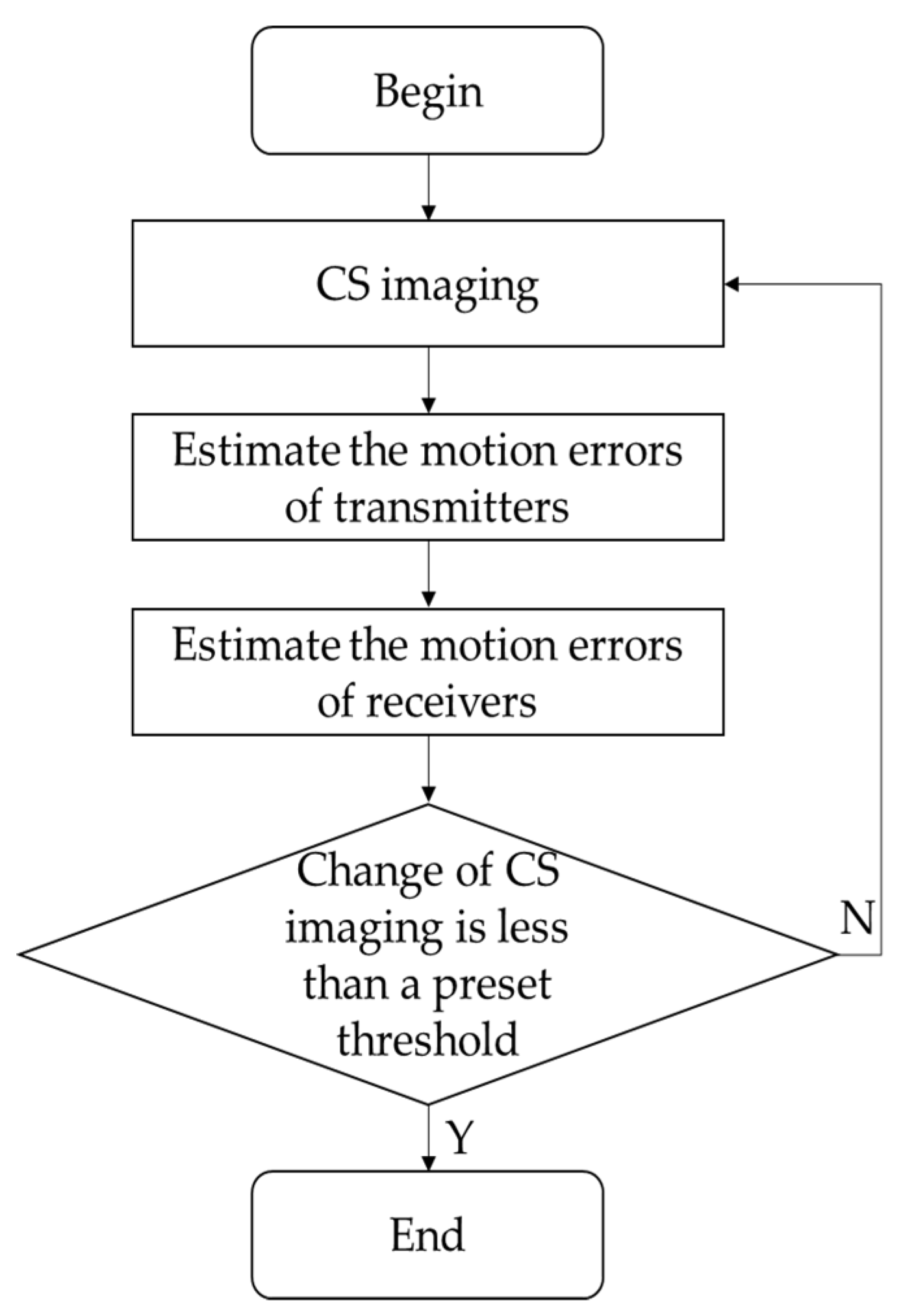
Because of the difference in propagation path, the method proposed in [30] for SAR cannot give an accurate estimation of array motion errors in MIMO situation. A BCD method is exploited to figure out (18), which cycles through steps of target reconstruction and array motion errors estimation and compensation. The algorithm flow is depicted as below. Figure 2 shows the flow chart of Algorithm 1.
| Algorithm 1 Compressed Sensing Imaging with Compensation of Motion Errors for MIMO Radar |
| Initialize:
, and return to step 1. is smaller than the presupposed threshold. |
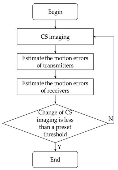
Figure 2.
Flow chart of Algorithm 1.
2.2.1. Target Reconstruction
In step 1, the targets are reconstructed with the given MIMO array motion errors. It can be depicted as
This type of problem can be figured out by sparse approaches, such as orthogonal matching pursuit (OMP) [37] or matching pursuit. We utilize OMP to get the reconstruction, considering that it can be utilized without knowing the data error magnitude in advance.
2.2.2. MIMO Array Motion Errors Estimation
In step 2, given the estimated receivers motion errors and the reflectivity coefficients vector in the iteration, the optimization problem is
On account of is a constant, (20) can be revised as
We depict the cost function by , and
where is the element in .
In (22), there are subprocesses in . In the subprocess, the cost function is only associated with the motion errors of transmitter , considering the estimated motion errors of receivers are provided here. Therefore, letting depict the subprocess as
To figure out (23), we use the gradient descent method. The gradient method is based on the assumption that the gradient can be calculated explicitly. We derive the gradient of according to . The gradient is as follows
The gradients are depicted as follows, utilizing the differential criterion of the composite function.
Using (2) and (3), we get
In (25)–(27), the calculation of is deduced in the Appendix A. Combining the equations from (25)–(30) and (A1), the explicit expression of the gradient can be accurately given. We can achieve the gradient of . A nesterov-accelerated adaptive moment (Nadam) [38] method is utilized to figure out (23). When (23) is solved, the global solution of (21) is given by taking the mean value, and step 2 in Algorithm 1 is realized.
Similarly, step 3 in Algorithm 1 is realized by the same means.
When the termination condition is fulfilled, the MIMO array transmits motion errors and receivers motion errors and the reflectivity coefficients can be estimated precisely.
2.2.3. Computational Complexity
We will analyze the computation complexity of each step respectively in this section. OMP is utilized in step 1 to reconstruct images, whose complexity is order , where depicts the number of targets. In step 2, the Nadam method is utilized to achieve the estimation of the MIMO array motion errors. Here, gradient computation dominates the computation complexity. The complexity of the gradient computation is order in each subprocess. Supposing there are sub iterations in step 2, the computation complexity of step 2 is . The computation complexity of step 3 is the same as step 2. Thereby, the computation complexity is in each iteration of Algorithm 1. Table 2 shows the complexity terms.
Table 2.
Complexity terms.
3. Results
3.1. Simulation
Table 3 shows the simulation parameters.
Table 3.
Simulation parameters.
Firstly, we place seven targets in the scene. Secondly, the MIMO array motion errors are simulated as uniformly distributed random errors, whose extent is of the wavelength. The fully sampled data are generated for BP imaging. To take advantage of the MIMO array information and make each subprocess have the same amount of data to achieve the estimation of the MIMO array motion errors, we used the following sparse strategy: use full of the transmitters and receivers; then randomly select the frequencies, whose indices are the same for each subprocess.
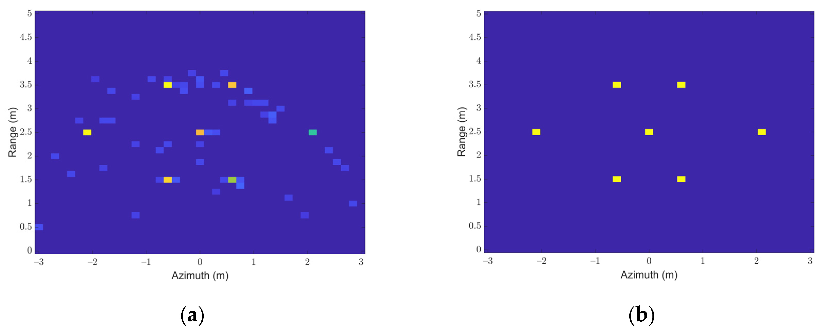
Figure 3 shows the contrast of imaging results without compensation of errors and the proposed method. Figure 3a shows the results without compensation of motion errors, which are defocusing on account of the array motion errors. In Figure 3b, the targets are reconstructed accurately by the proposed method.
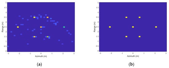
Figure 3.
Imaging Results Contrast. (a) Results without compensation of errors; (b) Results of the proposed method.
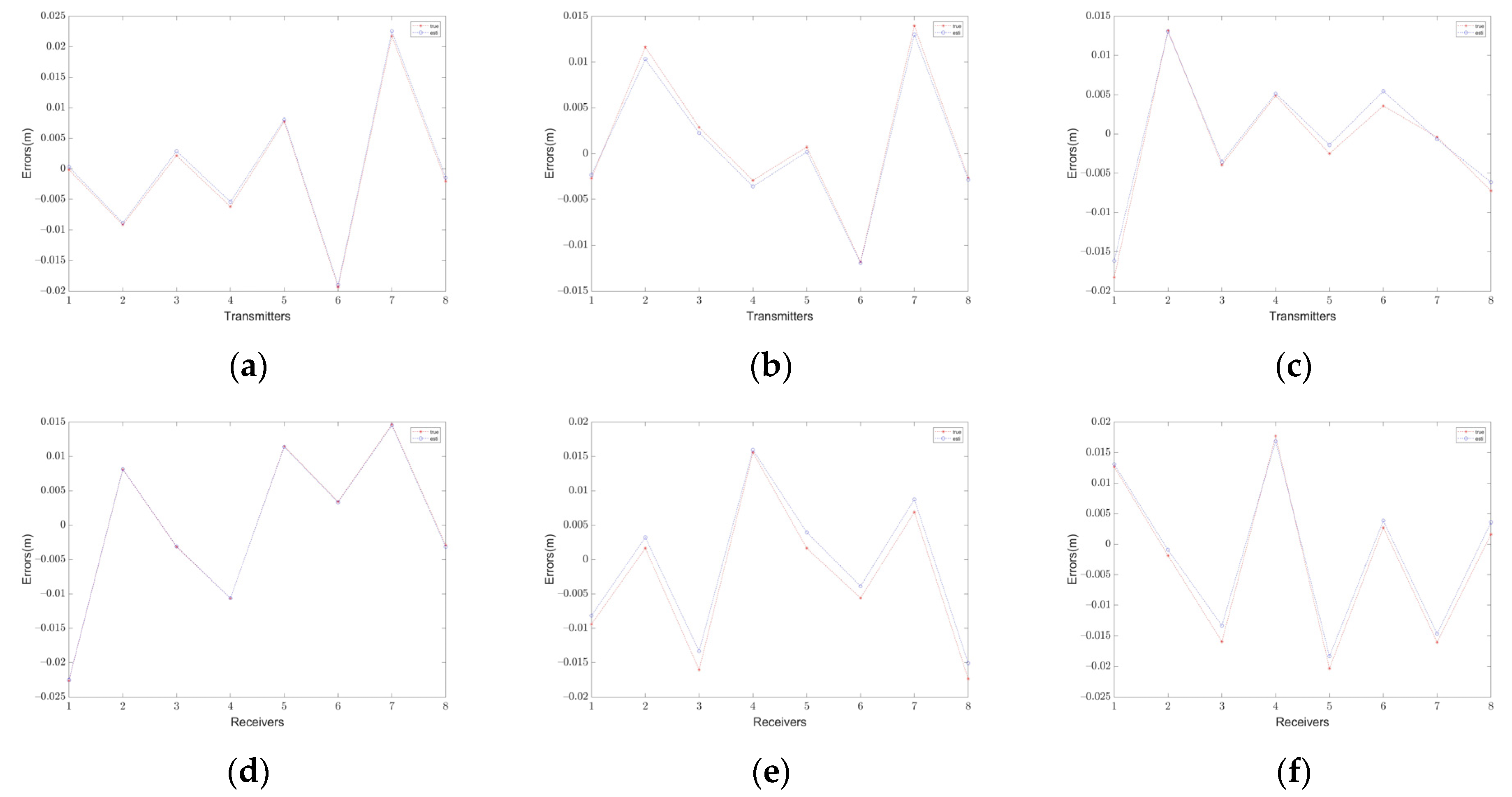
The estimation precision of the proposed method for MIMO array motion error is evaluated, and the superiority of this method is further emphasized. Figure 4 shows the true errors and estimated errors. Figure 4a shows the comparison between the error estimation results and the true error values of the dimension of the 8 transmitting array elements, where the horizontal coordinate represents the serial number of the transm−itting array. Figure 4d also shows the comparison between the error estimation result and the true error value of the dimension of the 8 receiving array elements, where the horizontal coordinate represents the serial number of the receiving array. Combined with Figure 4a,d the error estimation accuracy of the x dimension of the transmitting and receiving array is given. The remaining two columns depict the estimation precision in the and dimension, respectively. The results show that the estimation of errors of this method is in good agreement with the real errors.
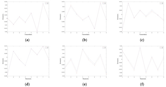
Figure 4.
MIMO array motion errors estimation. (a) dimension of Transmitters. (b) dimension of Transmitters. (c) dimension of Transmitters. (d) dimension of Receivers. (e) dimension of Receivers. (f) dimension of Receivers.
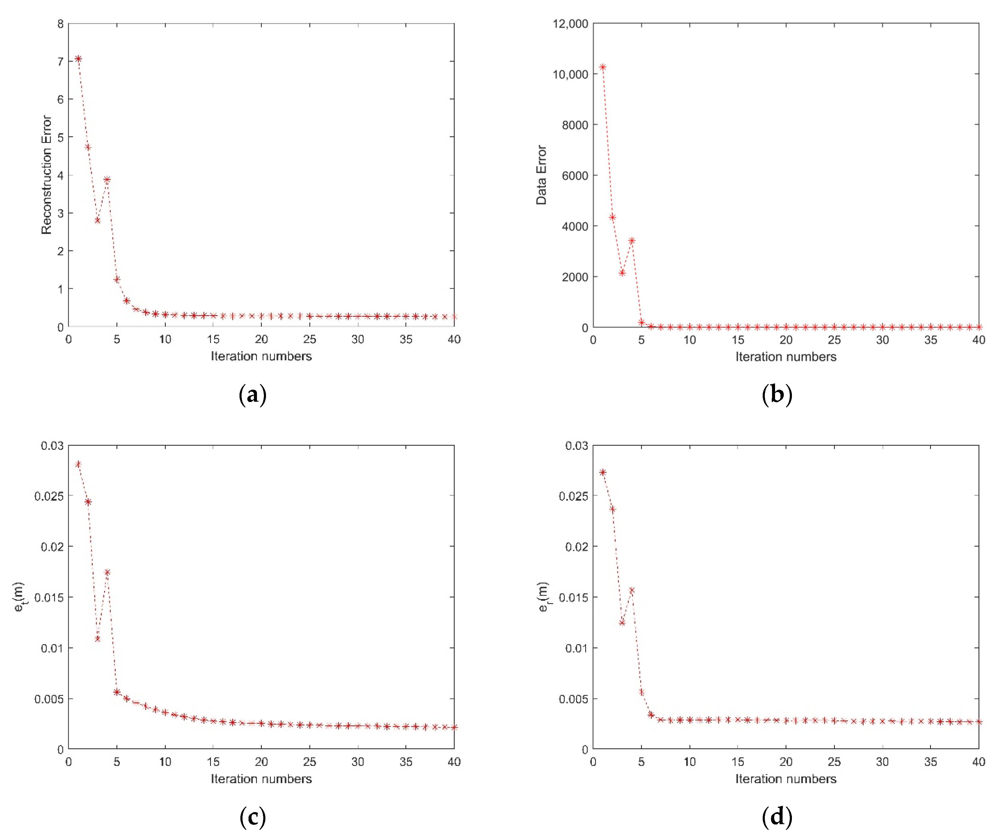
We define the data error as , where and are the MIMO array motion errors of transmitters and the receivers estimated at iteration , depicts the estimate of in the iteration. We define the target reconstruction error, i.e., , where depicts the actual value of . We define the root mean square error (RMSE) of the estimated errors as
where depicts the estimation of or in the iteration and depicts the true value of , denotes the number of transmitters or receivers.
In order to evaluate the convergence of the proposed method, the reduction of data error, reconstruction error, and RMSE of and in different iterations are illustrated in Figure 5. Since the change rate of the is less than the presupposed threshold, the method terminates at the iteration. The change of the target reconstruction error relative to different iterations is illustrated in Figure 5a. As the number of iterations increases to larger than 5, the target reconstruction error tends to zero. The change of the data error relative to different iterations is illustrated in Figure 5b. When the number of iterations is 5 or larger, the data error decreases and tends to zero. The quick reduction of RMSE of and are illustrated in Figure 5c,d respectively.
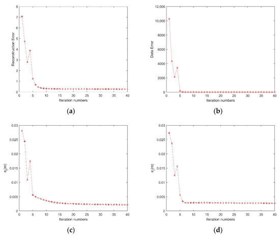
Figure 5.
Data error, Reconstruction error, and RMSE of and across the iteration. (a) Data error. (b) Reconstruction error. (c) RMSE of . (d) RMSE of .
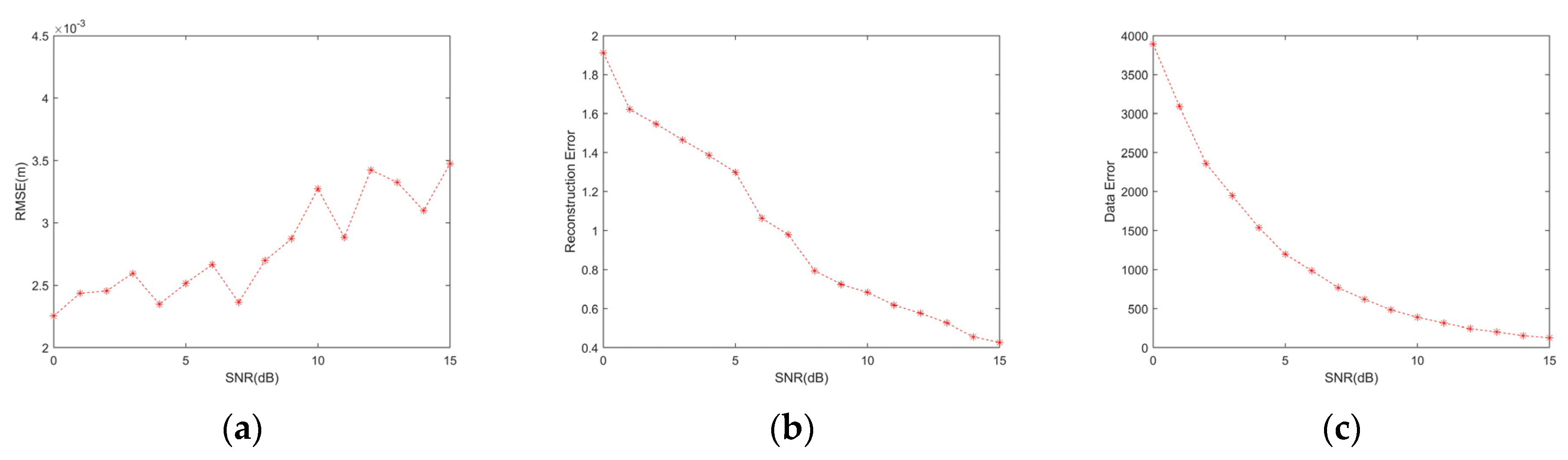
In addition, the robustness and accuracy to noise of the method are evaluated. Gaussian white noise with different SNRs is added to the original data, and 15 repetitions of the simulation were performed. The RMSE of all of the average estimated motion errors are less than 0.035 m under all simulated SNR conditions is illustrated in Figure 6a. In Figure 6b,c, if SNR is bigger than 6 dB, the target reconstruction error is smaller than 1 and the data error is smaller than 800. The simulations show that the method is robust to noise and has good reconstruction precision and estimation even under low SNR conditions.
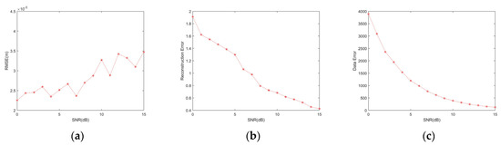
Figure 6.
Proposed method performance under different SNRs. (a) RMSE of the average of six directions motion errors. (b) Target reconstruction error. (c) Data error.
3.2. Experiment
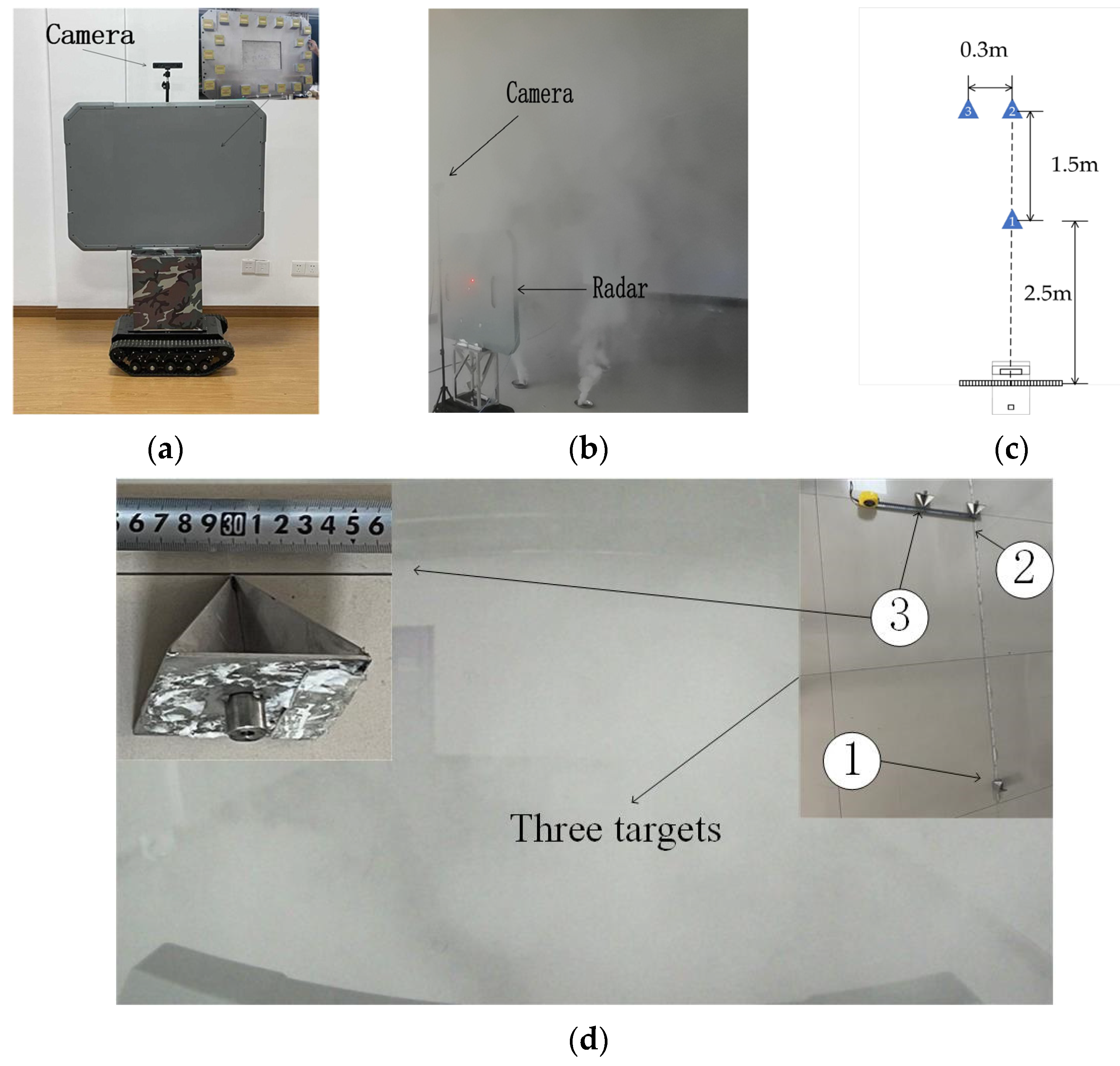
An MIMO radar with a stepped frequency waveform is installed on UGV for data collection in this experiment. The radar has 10 transmitters and 10 receivers. Figure 7a shows the details of the MIMO radar and the camera mounted above the radar. Figure 7b shows the radar and camera in an indoor artificial smoke scene. Figure 7c shows the diagram of corner reflector distribution. Figure 7d shows the optical image from the camera, in which the targets are invisible. The distribution of the three corner reflectors is illustrated with an additional optical image in the upper right corner of Figure 7d. The data from the reflectors is larger than the other areas, so the scenario can be seen as a sparse scenario. During the experiment, the UGV keeps moving. When the UGV passes by the designated position, the geometric center of target 1 is and the other two targets have geometric centers in and . The theoretical azimuth resolution is 0.36 m at a distance of 4 m. We first acquire the full data for BP imaging and utilizing part of the data for CS imaging. The experimental parameters are shown in Table 4.
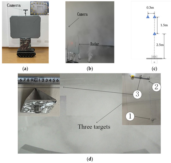
Figure 7.
Optical images of experimental scenes. (a) MIMO radar mounted on the UGV (b) UGV in the fog. (c) Diagram of corner reflectors distribution. (d) Optical images of three corner reflectors in a smoky scene.
Table 4.
Experimental parameters for MIMO radar.
A comparison of imaging results of different methods is illustrated in Figure 8. The BP imaging result is illustrated in Figure 8a. The result of conventional CS reconstruction without compensation of MIMO radar array motion errors is illustrated in Figure 8b. The result of the proposed method is illustrated in Figure 8c. Comparing with the optical image in Figure 7d, all the radar imaging results in Figure 8 show that the ability to perceive the environment has been significantly improved in a smoky scene. In Figure 8a, targets 2 and 3 are aliased together because the distance of the targets is small than azimuth resolution. In Figure 8b, targets one and two are defocused, which is owing to the effects of the radar array motion errors. In Figure 8c, the imaging quality is enhanced by compensating the motion errors so that targets 2 and 3 can be easily distinguished. It can demonstrate that the proposed method can achieve autofocus and super-resolution imaging.
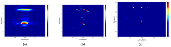
Figure 8.
MIMO radar experiments results. (a) Result of BP. (b) Result without compensation of errors. (c) Result of the proposed method.
4. Discussion
While the UGV-installed MIMO radar is moving, array motion errors are inevitable. In [29], a method is proposed to deal with the observation error under the SAR structure. A blind deconvolution method is proposed to acquire autofocus images [31], which can only solve the problem when antennas are influenced by the identical position error. Our proposed method can accurately estimate and compensate for the motion errors of the transmitters and receivers, as well as synchronously achieve autofocus imaging.
Figure 4 shows the estimation of motion errors is in good agreement with the true errors. Figure 8 shows that compared with traditional imaging method, the proposed algorithm can give super-resolution imaging in the presence of motion errors. In the smoky environment, the distribution of the targets can be accurately given by autofocus imaging, which has greatly improved the environmental perception ability compared with the optical sensor.
Future efforts will verify the validity of the method in complex environments such as the wild environment. Autofocus imaging of moving targets is a promising research direction in the future, which will increase the scope of the application of the algorithm. Incorporating low-rank and sparse for autofocus imaging may improve the noise suppression effect. Another research direction is considering the rigid constraints of the array during the estimating of array motion errors, which may be used to improve the speed and accuracy.
5. Conclusions
We have presented a method to compensate for the motion errors of the MIMO radar array in CS imaging. This method can realize the estimation of errors of the transmitters and receivers of the MIMO array and the reconstruction of the target image simultaneously. The proposed method analyses the essential relationship between the motion errors of array and the model. It uses a BCD iterative method, which iterates through target reconstruction, estimation, and compensation of the motion errors of the array. A gradient optimization method is utilized to get the estimation of the motion errors. The proposed method enhances the environment perception ability since it can accurately estimate the motion errors of the MIMO array and significantly improve the reconstruction results. The validity of the method is verified by simulation and measurement.
Author Contributions
Conceptualization, H.L. and T.J.; methodology, H.L.; software, H.L. and Z.L.; validation, H.L. and Y.D.; formal analysis, H.L. and S.L.; investigation, H.L.; resources, H.L.; data curation, H.L.; writing—original draft preparation, H.L.; writing—review and editing, H.L. and Z.L.; visualization, Y.D.; supervision, T.J.; project administration, T.J.; funding acquisition, T.J. All authors have read and agreed to the published version of the manuscript.
Funding
This research was supported in part by the National Natural Science Foundation of China under grant number 61971430.
Institutional Review Board Statement
Not applicable.
Informed Consent Statement
Not applicable.
Data Availability Statement
Not applicable.
Conflicts of Interest
The authors declare no conflict of interest.
Abbreviations
The following abbreviations are used in the manuscript:
| BCD | Block coordinate descent |
| BP | Back projection |
| CS | Compressed sensing |
| GPS | Global positioning system |
| INS | Inertial measurement units |
| ISAR | Inverse synthetic aperture radar |
| MIMO | Multiple-input multiple-output |
| Nadam | Nesterov-accelerated adaptive moment |
| OMP | Orthogonal matching pursuit |
| RCS | Radar cross section |
| RMSE | Root mean square error |
| SAR | Synthetic aperture radar |
| SNR | Signal noise ratio |
| UGV | Unmanned ground vehicles |
Appendix A
In this appendix, we will deduce the calculation of . Using (23), we have
Expand the absolute term in (A1) as
Then, we have
where
Using the expression of in (13), we have
References
- Czapla, T.; Wrona, J. Technology development of military applications of unmanned ground vehicles. Stud. Comput. Intell. 2013, 481, 293–309. [Google Scholar] [CrossRef]
- Bekkerman, I.; Tabrikian, J. Target detection and localization using MIMO radars and sonars. IEEE Trans. Signal Process. 2006, 54, 3873–3883. [Google Scholar] [CrossRef]
- Fischer, C.; Younis, M.; Wiesbeck, W. Multistatic GPR data acquisition and imaging. Int. Geosci. Remote Sens. Symp. 2002, 1, 328–330. [Google Scholar] [CrossRef]
- Bradley, M.R.; Witten, T.R.; Duncan, M.; McCummins, R. Mine detection with a forward-looking ground-penetrating synthetic aperture radar. In Detection and Remediation Technologies for Mines and Minelike Targets VIII; International Society for Optics and Photonics: Bellingham, WA, USA, 2003; Volume 5089, p. 334. [Google Scholar] [CrossRef]
- Ressler, M.; Nguyen, L.; Koenig, F.; Wong, D.; Smith, G. The Army Research Laboratory (ARL) synchronous impulse reconstruction (SIRE) forward-looking radar. Unmanned Syst. Technol. IX 2007, 6561, 656105. [Google Scholar] [CrossRef]
- Counts, T.; Gurbuz, A.C.; Scott, W.R.; McClellan, J.H.; Kim, K. Multistatic ground-penetrating radar experiments. IEEE Trans. Geosci. Remote Sens. 2007, 45, 2544–2553. [Google Scholar] [CrossRef]
- Jin, T.; Lou, J.; Zhou, Z. Extraction of landmine features using a forward-looking ground-penetrating radar with MIMO array. IEEE Trans. Geosci. Remote Sens. 2012, 50, 4135–4144. [Google Scholar] [CrossRef]
- Bilik, I.; Longman, O.; Villeval, S.; Tabrikian, J. The Rise of Radar for Autonomous Vehicles: Signal processing solutions and future research directions. IEEE Signal Process. Mag. 2019, 36, 20–31. [Google Scholar] [CrossRef]
- Cheng, Y.; Zhou, X.; Xu, X.; Qin, Y.; Wang, H. Radar Coincidence Imaging with Stochastic Frequency Modulated Array. IEEE J. Sel. Top. Signal Process. 2017, 11, 414–427. [Google Scholar] [CrossRef]
- Ciuonzo, D. On time-reversal imaging by statistical testing. IEEE Signal Process. Lett. 2017, 24, 1024–1028. [Google Scholar] [CrossRef] [Green Version]
- Ciuonzo, D.; Romano, G.; Solimene, R. Performance analysis of time-reversal MUSIC. IEEE Trans. Signal Process. 2015, 63, 2650–2662. [Google Scholar] [CrossRef]
- Devaney, A.J. Time reversal imaging of obscured targets from multistatic data. IEEE Trans. Antennas Propag. 2005, 53, 1600–1610. [Google Scholar] [CrossRef]
- Zhu, R.; Zhou, J.; Cheng, B.; Fu, Q.; Jiang, G. Sequential Frequency-Domain Imaging Algorithm for Near-Field MIMO-SAR with Arbitrary Scanning Paths. IEEE J. Sel. Top. Appl. Earth Obs. Remote Sens. 2019, 12, 2967–2975. [Google Scholar] [CrossRef]
- Gini, F.; Lombardini, F.; Montanari, M. Layover solution in multibaseline SAR interferometry. IEEE Trans. Aerosp. Electron. Syst. 2002, 38, 1344–1356. [Google Scholar] [CrossRef]
- Chen, C.; Xiaoling, Z. A new super-resolution 3D-SAR imaging method based on MUSIC algorithm. In Proceedings of the 2011 IEEE RadarCon (RADAR), Kansas City, MO, USA, 23–27 May 2011; pp. 525–529. [Google Scholar] [CrossRef]
- Donoho, D.L. Compressed sensing. IEEE Trans. Inf. Theory 2006, 52, 1289–1306. [Google Scholar] [CrossRef]
- Li, H.; Jin, T.; Dai, Y.P. Segmented random sparse MIMO-SAR 3-D imaging based on compressed sensing. In Proceedings of the IET International Radar Conference (IET IRC 2020), Online, 4–6 November 2020; pp. 317–322. [Google Scholar] [CrossRef]
- Suksmono, A.B.; Bharata, E.; Lestari, A.A.; Yarovoy, A.G.; Ligthart, L.P. Compressive stepped-frequency continuous-wave ground-penetrating radar. IEEE Geosci. Remote Sens. Lett. 2010, 7, 665–669. [Google Scholar] [CrossRef]
- Zhu, X.X.; Bamler, R. Tomographic SAR inversion by L1-norm regularization—The compressive sensing approach. IEEE Trans. Geosci. Remote Sens. 2010, 48, 3839–3846. [Google Scholar] [CrossRef] [Green Version]
- Zhang, L.; Qiao, Z.J.; Xing, M.; Li, Y.; Bao, Z. High-resolution ISAR imaging with sparse stepped-frequency waveforms. IEEE Trans. Geosci. Remote Sens. 2011, 49, 4630–4651. [Google Scholar] [CrossRef]
- Singh, K.B.; Arat, M.A.; Taheri, S. Literature review and fundamental approaches for vehicle and tire state estimation*. Veh. Syst. Dyn. 2019, 57, 1643–1665. [Google Scholar] [CrossRef]
- Guo, H.; Cao, D.; Chen, H.; Lv, C.; Wang, H.; Yang, S. Vehicle dynamic state estimation: State of the art schemes and perspectives. IEEE/CAA J. Autom. Sin. 2018, 5, 418–431. [Google Scholar] [CrossRef]
- Wahl, D.E.; Eichel, P.H.; Ghiglia, D.C.; Jakowatz, C.V. Phase Gradient Autofocus—A Robust Tool for High Resolution SAR Phase Correction. IEEE Trans. Aerosp. Electron. Syst. 1994, 30, 827–835. [Google Scholar] [CrossRef] [Green Version]
- Kolman, J. PACE: An autofocus algorithm for SAR. In Proceedings of the IEEE International Radar Conference, Arlington, VA, USA, 9–12 May 2005; pp. 310–314. [Google Scholar] [CrossRef]
- Yang, J.; Huang, X.; Jin, T.; Xue, G.; Zhou, Z. An interpolated phase adjustment by contrast enhancement algorithm for SAR. IEEE Geosci. Remote Sens. Lett. 2011, 8, 211–215. [Google Scholar] [CrossRef]
- Xi, L.I. Autofocusing of ISAR images based on entropy minimization. IEEE Trans. Aerosp. Electron. Syst. 1999, 35, 1240–1252. [Google Scholar] [CrossRef]
- Ye, W.; Yeo, T.S. Weighted least-squares estimation of phase errors for SAR/ISAR autofocus. IEEE Trans. Geosci. Remote Sens. 1999, 37, 2487–2494. [Google Scholar] [CrossRef] [Green Version]
- Cho, H.J.; Munson, D.C. Overcoming polar-format issues in multichannel SAR autofocus. In Proceedings of the 2008 42nd Asilomar Conference on Signals, Systems and Computers, Pacific Grove, CA, USA, 26–29 October 2008; pp. 523–527. [Google Scholar] [CrossRef]
- Liu, K.H.; Munson, D.C. Fourier-domain multichannel autofocus for synthetic aperture radar. IEEE Trans. Image Process. 2011, 20, 3544–3552. [Google Scholar] [CrossRef] [PubMed]
- Nguyen, M.P.; Ammar, S.B. Second order motion compensation for squinted spotlight synthetic aperture radar. In Proceedings of the 2013 Asia-Pacific Conference on Synthetic Aperture Radar (APSAR), Tsukuba, Japan, 23–27 September 2013; pp. 202–205. [Google Scholar]
- Kelly, S.I.; Yaghoobi, M.; Davies, M.E. Auto-focus for Compressively Sampled SAR. In Proceedings of the Keynote Speak of 1st International Workshop on Compressed Sensing Applied to Radar (CoSeRa 2012), Bonn, Germany, 14–16 May 2012. [Google Scholar]
- Du, X.; Duan, C.; Hu, W. Sparse representation based autofocusing technique for ISAR images. IEEE Trans. Geosci. Remote Sens. 2013, 51, 1826–1835. [Google Scholar] [CrossRef]
- Ender, J.H.G. Autofocusing ISAR images via sparse representation. In Proceedings of the 9th European Conference on Synthetic Aperture Radar, Nuremberg, Germany, 23–26 April 2012; pp. 203–206. [Google Scholar]
- Yang, J.; Huang, X.; Thompson, J.; Jin, T.; Zhou, Z. Compressed sensing radar imaging with compensation of observation position error. IEEE Trans. Geosci. Remote Sens. 2014, 52, 4608–4620. [Google Scholar] [CrossRef]
- Pu, W.; Wu, J.; Wang, X.; Huang, Y.; Zha, Y.; Yang, J. Joint Sparsity-Based Imaging and Motion Error Estimation for BFSAR. IEEE Trans. Geosci. Remote Sens. 2019, 57, 1393–1408. [Google Scholar] [CrossRef]
- Mansour, H.; Liu, D.; Kamilov, U.S.; Boufounos, P.T. Sparse Blind Deconvolution for Distributed Radar Autofocus Imaging. IEEE Trans. Comput. Imaging 2018, 4, 537–551. [Google Scholar] [CrossRef] [Green Version]
- Tropp, J.; Gilbert, A. Signal recovery from random measurements via orthogonal matching pursuit. IEEE Trans. Inf. Theory. 2007, 53, 4655–4666. [Google Scholar] [CrossRef] [Green Version]
- Dozat, T. Incorporating Nesterov Momentum into Adam. In Proceedings of the 4th International Conference on Learning Representations, Workshop Track, San Juan, Puerto Rico, 2–4 May 2016; pp. 1–4. [Google Scholar]

Publisher’s Note: MDPI stays neutral with regard to jurisdictional claims in published maps and institutional affiliations. |
© 2021 by the authors. Licensee MDPI, Basel, Switzerland. This article is an open access article distributed under the terms and conditions of the Creative Commons Attribution (CC BY) license (https://creativecommons.org/licenses/by/4.0/).