1. Introduction
Of the 820 million undernourished people worldwide, most are living in Africa [
1] with poverty and global warming contributing to the ever-worsening scourge of malnutrition. This situation calls for additional research into staple crops that are well adapted to the tropics, tolerate erratic weather, and thrive even in drought and low-input farming systems. No other crop is more suitable for this purpose than cassava. Cassava (
Manihot esculenta Cranz) is the richest and cheapest source of carbohydrates and produces higher amounts of starch per unit area compared to other staple crops [
2]. Producing cassava requires few inputs and affords farmers great flexibility in terms of timing the harvest, as the crop can be left in the ground even after reaching physiological maturity [
3]. Cassava’s tolerance to erratic weather conditions, including drought, makes it an important component of climate change adaptation strategies [
4,
5]. Breeding efforts to biofortify cassava with vitamins have been fruitful [
6], further making it an ideal staple crop to reduce malnutrition, hunger and poverty. As a result of the crop’s multipurpose use and adaptability to harsh environments, it has been described as the “drought, war and famine crop of the developing world” [
7].
According to market research [
8] it was reported that the global cassava-processing market reached a volume of ~300 million tons in 2020, demonstrating the global importance of the crop. Worldwide production of cassava amounted to ~300 million metric tons in 2018 of which Africa’s share was 67% [
9]. In the same year, Nigeria alone produced 56 million metric tons, comprising 28% of the production in Africa and 18.5% of the global production. As an annual crop, cassava is generally harvested 12 months after planting. There is currently a lack of varieties that are capable of producing profitable root yield in terms of quality and quantity at fewer months after planting [
10,
11,
12]. Early bulking is a trait term that is used to describe early maturity in cassava. According to the cassava trait dictionary called “Ontology”, early bulking is defined as the time taken for storage roots to begin to accumulate and store starch in the root [
13]. In this paper, early storage-root bulking is denoted as ESRB.
Under normal economic and environmental constraints, African farmers cannot afford to wait 12 months before harvesting the crop. Late storage root bulking is not defined in the ontology but is used herein to describe varieties that are not bulking prior to 12 months. Early harvest of late storage root bulking varieties (which is a characteristic of most local and improved varieties) leads to low productivity. ESRB is a crucial trait required by farmers as it is critical to the crop’s role in food security for sub-Saharan Africa [
14]. Reports from recent participatory rural appraisals in Nigeria indicated that farmers reject some improved varieties because of the length of time it takes to achieve maturity [
15,
16,
17]. Thus, farmers must be provided with knowledge of early bulking and the advantages it offers. Moreover, results from surveys across Africa have amplified the importance of the ESRB trait. For instance, in Uganda, ESRB was second only to high yield as a desirable attribute. Farmers discovered that early bulking genotypes escape late season pests, diseases and droughts, allowing for sequential multiple cropping within one cassava cropping season. They also contain lower cyanogenic compounds, and above all, they provide rapid food and income [
17]. In semi-arid areas, ESRB is crucial as it permits harvesting after only one cycle of rain or immediately after a second rainy period.
Despite the importance of ESRB, there is a paucity of research efforts to improve the trait for utilization by breeders. In order to achieve tangible progress in the improvement of the ESRB trait in cassava, there is an urgent and pertinent need to reduce the difficulties encountered in phenotyping. There currently exists no morphological or visual system that allows breeders to recognize when a cassava plant starts accumulating starch in the root system outside of harvesting the roots, thus making it difficult for breeding programs to identify early bulkers without intense labor. Presently, phenotyping of ESRB is carried out using manual, destructive sampling methods [
18,
19] which are time consuming. In addition, due to the length of the bulked roots underground (which could reach up to 2 m), excavation and measurement become cumbersome and prone to inaccuracies and biases, making destructive sampling methods unsuitable for screening large genetic populations [
20]. Non-destructive root sampling methods would allow for repeated measures of the same plants or plots and enable smaller, more efficient trials that require fewer planting materials. Therefore, there is a need for research on novel rapid, non-destructive methods to phenotype ESRB in cassava. Such methods, once developed and implemented, will permit increased precision in the selection of the best genotypes, saving time and scarce resources [
21].
Ground-penetrating radar (GPR) has established itself in numerous geoscience, civil engineering (including non-destructive detection of moisture in concrete [
22,
23]), archeology, glaciology and military applications [
24]. However, the technique has yet to make a widespread impact on agricultural science, though it has seen use in related studies of forest ecosystems and other environmental applications [
25,
26]. GPR has previously been used to detect the roots of different plant species [
27,
28], being performed on trees [
28,
29,
30], cassava [
31,
32] and peanut plants [
33]. However most of the studies were either conducted in controlled environments or were based on simulated data in order to evaluate signal processing algorithms [
28]. Liu et al. [
29] investigated the use of GPR in the detection of fine roots (<2 mm in diameter) based on a radargram analysis technique called pixel index selection. Significant relationships were detected between the GPR pixel indices and root parameters.
However, only a few evaluations of GPR for the detection of root biomass in cassava breeding trials have been conducted. Delgado et al. [
31] considered supervised root biomass estimation in cassava based on image thresholding. The locations of roots in the soil along the radar-scan transect were determined after scanning. Radargrams from the specifically identified areas were then analyzed to choose the best threshold, thereby making the method “supervised”. The aboveground vegetation was cleared before scanning to allow for ease of movement of the GPR device in the field. Destructive sampling was also performed as the roots were excavated from the soil after scanning. Delgado et al. [
32] also investigated cassava root biomass determinations based on variations in root sizes buried at different positions in the soil during a controlled experiment. The study was conducted in a large box of pure sand using a computer numerical control (CNC) machine to ensure spatially uniform GPR data acquisition. However, agricultural experiments performed in actual soils are always characterized by heterogenous field conditions.
The objective of this study was to evaluate the use of ground-penetrating radar (GPR) as a non-destructive method for predicting cassava root biomass and selection of ESRB, in particular, using a cassava breeding trial with 7 planting dates. The study demonstrates the capability of GPR for rapid phenotyping of root biomass and suggests that use of GPR can be an effective new tool for breeding and selection of ESRB in cassava.
2. Materials and Methods
2.1. GPR Operating Principles and Visualization Mode
GPR is a geophysical tool used for exploring the subsurface of the earth to depths ranging from several cm up to several km under ideal conditions [
34]. The method involves a transmitter emitting a very short (nanosecond-scale) pulse of electromagnetic energy (EM) along with a receiver “listening” for subsurface reflections. The instrument measures the amplitude and the travel time of the reflected energy (
Figure 1), with reflections being caused by changes in the relative dielectric permittivity of the material through which the wave propagates. Relative permittivity describes the ability of a material to alternately store and release EM energy in the form of bound charge polarization [
35]. Besides reflection, the emitted signal can also be scattered, transmitted, refracted, diffracted and absorbed [
34]. Only a small portion of the scattered wave energy is measured (i.e., the back-scattered component), while refracted waves may or may not be captured by the receiving antenna. Transmitted waves are lost unless they are reflected toward the surface receiver by deeper layers or buried targets. Absorbed energy is thermally dissipated throughout the medium, resulting in signal attenuation [
34,
36].
The GPR detection threshold (or resolution) and penetration depth are both inversely related to the central frequency of the EM pulse spectrum. This is the well-known range-resolution tradeoff [
37]. Increasing frequency improves the detection threshold, such that smaller objects can be detected while larger objects have better definition; but higher frequencies also leads to greater signal attenuation and hence reduced range [
38]. In general, the smallest object for which a discrete signal return can be discriminated must have a characteristic size of at least ¼ of the predominant signal wavelength. The latter is defined by the central frequency of the pulse spectrum but also by the electrical characteristics of the medium through which the wave is traveling; primarily, the relative permittivity. The latter is chiefly dependent on water content [
37]. Thus, the minimum detection threshold in GPR agricultural applications varies with soil water content. Increased soil moisture results in improved detection capabilities (shorter wavelengths), but reduced penetration depth. In each application, the range-resolution tradeoff must be taken into consideration when selecting an appropriate GPR configuration [
34].
2.2. Radar Acquisition Device
GPR data were collected using an experimental GPR prototype system developed by IDS Georadar (Pisa, Italy) consisting of a tablet computer, radar electronics (signal emitter, processing unit, etc.), antenna array and field cart. The antenna array can be classified as an air-launched, bistatic configuration of modified vee-dipole wideband 1.8-GHz vertically-polarized antennas [
39,
40]. The array consists of 8 antennas, each separated by 4 cm, with alternating transmit and receive capability. The array is housed in a 3D-printed box, with EM absorbing material placed above the antennas to protect them from stray electromagnetic fields induced in the cables. The box is mounted beneath a 2-wheeled cart which is shaped somewhat like a bicycle, and pushed from behind. The bottom of the box is ~30 cm above the ground surface, and can be angled to either side up to 40° from nadir. An encoder wheel maintains contact with the larger of the cart wheels to measure the distance traveled, and pulses are emitted every 1 cm of travel, each one triggering a GPR response measurement. The tablet computer runs the acquisition software K2Fastwave (IDS Georadar, Pisa, Italy). This software allows the user to configure certain aspects of the GPR system, such as signal stacking and transmit/receive channel pairing. The system is capable of collecting data as quickly as 4500 m per hour, though increasing the number of channels and the amount of signal stacking slows down acquisition in most cases. A number of studies [
33,
37] have been conducted using the vee-dipole antenna type and reports from these tests reveal the suitability of the antenna type for agricultural-related GPR experiments.
2.3. Cassava Trial
The study was conducted on a field trial at the International Institute of Tropical Agriculture (IITA) in Ibadan, Nigeria. The site location is latitude 7.388 N, longitude 3.896 E, altitude 227 m, with the land type being derived Savanna (i.e., forest land that has been cleared for cultivation). The annual rainfall is 1260 mm, with average temperature range of 20.7 to 33.8 °C, and 238-day growing period. There are two rainy seasons, from March to July and from mid-August to November. The soil at the study area is Ferric Luvisol.
2.4. Field Design and Planting
Land preparation included mowing, discing, harrowing and ridging by tractor. Cassava stakes (the planting material) were hand planted by burying 25 cm cassava stems in the soil slanted at a 45-degree angle with 5 cm of the stem aboveground. Each stake had approximately 25–30 nodes. Each plot consisted of 5 rows 4.8 m in length with 1.0 m between rows. Within row planting distance was 0.8 m for a total of 30 plants per plot. Three cassava genotypes, TMEB419, TMEB693 and IBA070539, were sourced from IITA germplasm. Two of the genotypes are white-fleshed (TMEB419 and TMEB693), while IBA070539 is yellow-fleshed. The genotypes were planted using a complete block design with 3 replications at one location. Testing was performed during the 2018/2019 growing season. Root morphology data were taken from each plot on the net plot area of 12 plants excluding plants in border rows and at the end of each row.
A staggered planting design based on seven different planting times (time of the year cassava stakes were planted) was used, with genotypes planted between June and August 2018 at 4 weeks intervals. Subsequently, harvesting was performed at one period from 22–26 April 2019. There were 3 replications and each consists of 21 plots with each genotype replicated seven times. A replication consists of three blocks, one for each genotype (
Figure 2).
2.5. Field Data Collection
From the five available rows, only the inner rows 2, 3 and 4 were scanned by the GPR, the instrument being pointed respectively in the eastern and western directions in two passes. Along each row, the first pass started from the beginning of the plot in the first replication and ended in the third replication, while the second pass started from the third and ended in the first replication. In this manner, GPR scans covered both sides of each row. The antenna array is configured such that an electromagnetic pulse is sent by a transmitting antenna at time 0 ns and a receiving antenna records the voltage of the returned signal within an 18 ns time window during which 512 samples are recorded [
33]. A total of 378 GPR transects (3 rows in 7 plots of 3 replications in 2 passes for 3 genotypes) were collected (see
Figure 2 for the trial layout).
The branching habit (
Figure 3) of cassava, however, poses a challenge in maneuvering the GPR cart along the alley and between rows in the field. Cassava has different branching habits as described in the breeding database [
41]. Visual rating of branch height is conducted on a scale of 0 = no branching, 1 = low branching (<0.5 m), 2 = medium branching (>0.5 m and ≤1 m), 3 = high branching (≥1 m) [
42]. Cassava plants with a high branching habit are considered to produce good yield, good leaves and long leaf life since the number of shoot apices per plant is determined by the degree of branching [
43].
2.6. GPR Data Processing
GPR data processing was performed using GPR-Studio version 1.0.1, a web-based application software [
44]. Common processing methods previously used in GPR studies in agriculture [
31,
32,
33] were considered and combined for testing. Of the six channels of data collected, only one channel was used in this analysis because of excessive noise in the other channels. The entire radargram (B-scan) was used except the portion affected by the direct wave and ground clutter. Thus, the muted B-scan includes information from the air (from antenna to the ground) and the subsurface beneath the clutter-affected zone. Next, coherent sub-horizontal reflected energy was mitigated using a background correction. Kirchoff migration was then performed to collapse diffracted-energy tails to their representative points of origin. The Kirchoff parameters used were identical to the ones used in [
33]. A schematic representation of the workflow is shown in
Figure 4.
Four different GPR data-processing pipelines were tested (
Table 1) using various combination of the methods shown in
Figure 5 and
Table 1.
2.7. Feature Extraction
A discrete Fourier transformation (DFT) was performed on the A-scans to convert the GPR data from time to frequency domain. The DFT estimates the complex Fourier coefficients over a range of frequencies as described by [
45]. The squared amplitude of the Fourier coefficients comprises the power spectrum which is a measure of the amount of signal power that lies within each frequency bin. The power spectrum indicates the contribution of each frequency component to the signal power (
Figure 6). Since multiple B-scans are acquired in the two GPR scans of each plot, so that there was some data redundancy, the power spectra were averaged to improve the signal-to-noise ratio. The GPR response of a plot is thereby represented by an m x n matrix of average GPR signal power, where m represents the rows (3 rows) and n, the number of frequency bins. In total, there are 189 rows of data from the 63 field plots.
Only those Fourier coefficients in the range 0.35–2.78 GHz were analyzed, this decision being based on the central frequency of the GPR instrument (1.8 GHz). Rows with more than 2 of 4 dead plants (≥75% missing plant stands) were removed from the dataset. The removal was done to reduce any bias (such as noise or gaps left by dead roots) that might have been introduced as a result of modifications to the soil environment before the plants died. A total number of 170 rows (~90% of the original dataset) were then considered for further statistical analysis.
2.8. Test for Difference in Planting Time
In order to evaluate differences in maturity using the staggered planting time trial, an analysis of variance (ANOVA) was carried out on the raw phenotypic data using the generalized linear model (GLM) procedure of the software package Statistical Analytical System (SAS 9.4, Cary, NC, USA). The mean squares (MS) resulting from the analysis (
Table 2) represent the variance components for each of the explanatory variables derived by dividing sum of square of the variation (SS) by the degree of freedom (DF).
Table 2 presents the ANOVA results for root biomass evaluation in Ibadan. The MS for planting time is highly significant based on the probability (
p < 0.0001) associated with F-statistics; showing there is a difference in bulking with respect to time of planting. This variable captured 42.7% of the variation in root biomass. Other explanatory variables such as genotype and replication are also highly significant (
p < 0.0001) capturing 34.1% and 21.3% of the variation in root biomass, respectively. The effect of row was not significant (
p < 0.8297), however, capturing 0.29% of the variation in root biomass.
2.9. Statistical Analysis
Table 3 shows the 6 regression models that were evaluated in terms of their ability to predict root biomass. The latter serves as the response variable while the functional covariates listed in the second column are the predictors.
A recent study [
46] shows the power and utility of functional regression models in high-throughput phenotyping studies. Functional regression within a Bayesian framework is used herein with all model parameters being assigned a prior density reflecting their uncertainty [
47]. Prediction is based on the Bayesian ridge regression (BRR) method as described by [
48,
49] as implemented in the R package BGLR (a total of 20,000 Markov chain Monte Carlo iterations were used, with the first 5000 discarded as burn-in) [
50]; however, in this study, GPR features are used instead of molecular markers.
The BRR method assumes weak priors for the beta coefficients (regression coefficient ) of each covariate. This is achieved by assuming that each beta coefficient obeys the distribution N(0, and (prior for the variance of beta coefficients), where denotes the scaled inverse Chi-squared distribution with shape parameter and scale parameter .
The six Bayesian models were tested using the phenotypic data and the GPR power spectra using a single-step functional regression model.
The design matrix of the GPR power spectrum, denoted by X, is introduced into the BRR model as an approximation of the experimental plot P. The vector of the power spectrum random effect is assumed to obey x ~ N(0, X ) where is the variance component of power spectrum and X is the scaled power spectra relationship matrix computed using the matrix of power spectra (M) from the GPR data of order P × as X = MMT/. The design effects (row, replication and genotype) and their interactions with X were considered to be functional covariates in all the models.
Below is the list of the BRR modelling equations (Equations (1)–(6)).
Models without interaction
Model with interaction of the design effects
Model with interaction of the design effects and power spectrum covariates
Design matrices were reconstructed for all explanatory variables using the interactions with matrix of X: , and in models 3 and 4, as follows:
Next, the explicit description of model 4 explained in Equation (6) is presented.
In the above equations, is the response variable (root biomass) corresponding to the kth genotype, jth replication and ith row, while µ is the overall mean. The variable is the random effect of the ith row distributed ~ N(0,) where is the row variance component, is the random effect of the jth replication with ~ N(0,) where is its variance component. The variable is the random effect of the kth genotype with ~ N(0,) where is the genetic variance component. The variable is the interaction term between replication and row distributed as ~ N(0,) with as the variance component. The variable is the interaction term between replication and genotype distributed as N(0,) with as the variance component. The variable is the interaction between GPR power spectrum and genotype distributed as N(0,) with as the variance component. The variable is the interaction between GPR power spectrum and row distributed as N(0,) with as the variance component. The variable is the interaction between GPR power spectrum and genotype distributed as N(0,) with as the variance component. The variable is the three way interaction between GPR power spectrum, replication and row distributed as N(0,) with as the variance component. The variable is the three-way interaction between power spectrum, replication and genotype distributed as N(0,) with as the variance component and is an error term distributed as .
It is important to point out that by deleting certain terms in Equation (6), the remaining models described in Equations (1)–(5) can be obtained.
2.10. Cross Validation Scheme
A K-fold cross validation scheme was used as a resampling procedure (where K is the number of groups or subsets called “folds” into which the dataset will be divided into). The scheme was considered because the folds are mutually exclusive; this helps to avoid overfitting and better model generalization. A five-fold cross validation scheme was used wherein plots were randomly subdivided into five mutually exclusive subsets. Four subsets were used as a training set while the remaining subset is used as the validation set. The same procedure was repeated five times to ensure prediction accuracy estimates would be significant for the improvement of breeding activities. This is important especially in early-stage testing where large numbers of genotypes are screened in unreplicated plots. For each of the GPR data processing pipelines and each of the BRR models tested within the pipelines, twenty-five prediction accuracies (r), coefficients of determination (R2) and normalized root mean square errors of prediction (NRMSEP) were generated. In addition, the average and standard error (SE) estimate of the prediction accuracy and NRMSEP were estimated.
The prediction accuracy was defined in terms of the Pearson correlation between the observed and predicted root biomass. Prediction accuracy and NRMSEP (equation [
8]) are used as metrics for evaluating the prediction performance; where
is the predicted root biomass and
is the observed root biomass. The higher the prediction accuracy, the better the model and the lower the NRMSEP value.
The standard error of the prediction accuracy and NRMSEP is calculated as:
All statistical analysis was performed using R statistical software version 3.5.2 (R Core Team, 2018)
3. Results
Prediction accuracy results from the 5-fold cross validation scheme with five repetitions showed that a combination of GPR power spectra and field design effects acting as functional covariates can significantly improve prediction of cassava root biomass to correlation as high as r = 0.72 (
Figure 7). Results from all the data processing pipelines (P0 to P3) and Bayesian models (Baseline to M4) showed that prediction accuracy increases if GPR spectra are introduced as a covariate. The boxplot in
Figure 7 displays the distribution of the Pearson correlation: P3 has the highest prediction accuracy, followed by P2, P0 and P1. Similarly, model 1 had the highest accuracy, followed by model 0, model 4, model 3, model 2 and Baseline.
As shown in
Table 4, combining GPR power spectra with the other field design effects as functional covariates significantly improves the prediction of cassava root biomass, with up to 26% explained variation (R
2 = 0.26 for model 1 and pipeline 3). Prediction increased by up to 17% explained variation for models including GPR power spectra and field design effects compared to the baseline model. Adding field design effects to GPR power spectra slightly increased the explained variability, but including interaction terms does not increase model accuracy. With respect to GPR processing methods—using the raw GPR data (R
2 = 0.19) or background correction (R
2 = 0.19) and migration (R
2 = 0.18) alone produced similar accuracy. The migration-only pipeline slightly decreased the explained variability. The best explained variability is achieved when background correction and migration were applied together (R
2 = 0.26).
3.1. GPR Processing Methods
The boxplot distribution of the prediction accuracies of the four GPR processing methods (
Figure 7) showed good results for models 0,1 when using background correction and Kirchoff migration (P1, P2 and P3). The preprocessing methods generally improve prediction accuracy, while a comparison between pipeline 1 and pipeline 3 revealed the importance of combining Kirchoff migration with background correction.
3.2. Models
To evaluate the effect of functional covariates in predicting root biomass, six different Bayesian models were constructed (
Table 3). A comparison of models with and without using GPR power spectra as a covariate indicated that the prediction accuracy and R
2 was higher, while NRMSEP was lower in all models that included GPR spectra (
Table 4). For example, comparing the Baseline and model 1 showed that including GPR spectra increases R
2 by ~52% and r by ~30% while reducing NRMSEP by ~5.5% across all GPR processing methods except for pipeline 3, which combined Kirchoff migration and background correction. In that case, R
2 increased by 189% and r by 48%, with NRMSEP being reduced by 10%. A further comparison between model 2 and model 4 showed a similar trend: R
2 increasing by ~42.8% and r by ~26.3%, with NRMSEP reducing by ~4.1% across all the methods (
Table 4).
Based on the findings from the cross-validation scheme discussed above, the models for root biomass prediction using GPR power spectra with pipeline 3 in a non-cross validation scheme were compared. The result shows that models with GPR spectra as a covariate outperformed those without.
Figure 8 shows that 41% of the variation in root biomass is explained (R
2 = 0.41), with a Pearson correlation coefficient (r) of 0.64 for model 1 (see
Figure 9 for other models). The results provide evidence that the GPR power spectra contains information about cassava root structure, and that a simple regression model without interactions between covariates (M1) produces the best mean prediction accuracy from both the cross validation and non-cross validation schemes.
4. Discussion
Research has shown the importance of the ESRB trait in cassava, a major crop that supports food security in sub-Saharan Africa [
14]. The ability to predict root biomass, especially in early-stage trials but also in practice on farmers’ fields, cannot be over-emphasized. Selection for the ESRB trait would allow sequential multiple cropping within a single growing season [
17] and also allow rapid multiplication of planting materials through rapid selection and identification of advance clones that have bulked early and gained appreciable root biomass.
In agricultural research centers, one of the essential mandates is to deliver improved varieties to farmers. In new product designs, ESRB becomes an essential trait. Breeders might have identified parents for hybridization purposes within a population improvement plan; however, phenotyping the trait may still pose a challenge. Thus, the use of GPR as a tool to rapidly estimate root biomass can be used to facilitate rapid phenotyping.
Our result agrees with previous findings of [
31] that root biomass can be predicted using GPR. This assessment is based on the prediction accuracies reported herein in
Table 4 and
Figure 7. However, the predictive power reported in [
31] turned out to be higher. To achieve its stronger correlations, the previous work relied on destructive techniques and a supervised processing such that the precise position of roots was determined prior to GPR data processing. As further research is completed, the explanatory power of GPR spectra should become better understood and the predictive power based on the approach described in this study is expected to improve. In addition, the current GPR cart design introduces antenna positioning to target root errors when scanning lowly branched genotypes.
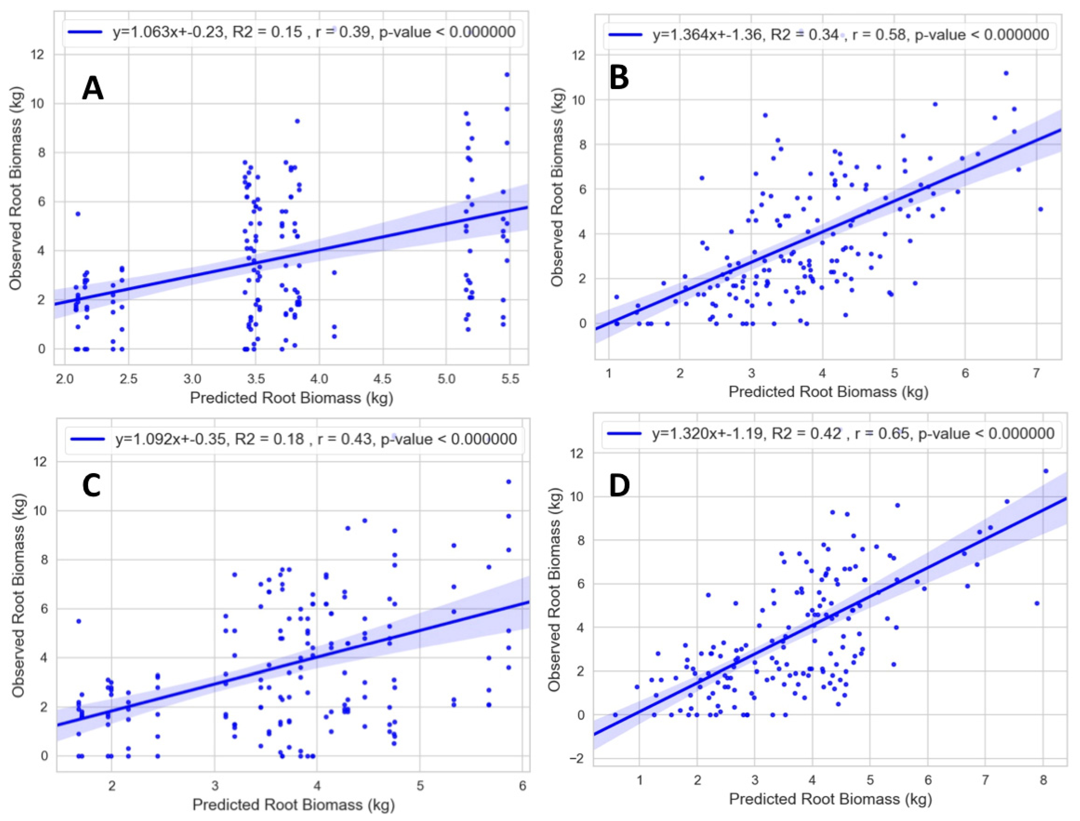
Figure 8 and
Figure 9 shows how the Pearson correlation coefficient r and coefficient of determination R
2 depend on the regression model, based on a non-cross validation scheme. A visual comparison of the scatter plot diagrams shows that models that do not use GPR power spectra look “binned” and deviate significantly from the regression line. According to
Figure 8, model 1 shows an increase in the prediction accuracy (r = 0.64) over the Baseline model (
Figure 9A), explaining 41% proportion of variation in root biomass (R
2 = 0.41).
Figure 9B shows that using GPR power spectra alone (model 0) explains 34% of the variation in the root biomass (R
2 = 0.34) with a prediction accuracy of (r = 0.58). This finding indicates that the GPR power spectra contain valuable information about cassava root structure.
There is no significant difference between the regression modeling results of Baseline and model 2 (
Figure 9C). The lack of discernment is not surprising, as the design effects modelled in Baseline can explain only 15% of the variation in root biomass (R
2 = 0.15) with a prediction accuracy of (r = 0.39), while model 2 explains only 18% of the variation in root biomass (R
2= 0.18) with a prediction accuracy of (r = 0.43).
Model 4 (
Figure 9D) shows that the design effects along with the interaction terms explain 42% of the variation in root biomass (R
2 = 0.42) with a prediction accuracy of (r = 0.65), which is only slightly different from the proportion explained by model 1. From the result shown in
Table 4, there is an indication that model 4 might be over-parameterized for prediction. Our results suggest that a regression model incorporating a few main effects without interaction terms should prove sufficient.
Introduction of genotype effect as a functional covariate was used to adjust the predicted root biomass for the branching habit exhibited by the genotype. Genotype and branching habit are synonymous because there is no variation in the branching score for each of the genotypes as such: TMEB419 has a visual rating of “0”, IBA070539; “1” and TMEB693; “2” throughout the experiment [
42].
The efficiency of the prediction model described in this study can be vastly affected by a noise in the GPR spectra. The data processing methods used in this study (included in the pipelines 0–3) are aimed to rectify and denoise the GPR responses. Liu et al. [
33] suggested that a strongly heterogeneous subsurface may enhance signal attenuation. It should be noted that agricultural trial sites are often strongly heterogeneous, potentially reducing the positive impact of GPR responses on phenotyping capability. Further to this, GPR responses become more complicated and perhaps less predictive if the branching habit of the genotype is short and “umbrella” in shape. In simple terms, lowly branching genotypes create GPR data acquisition errors due to antenna targeting of roots being impaired. However, technology advancement may help address data acquisition ambiguities and uncertainties. For example, if the antenna array is embedded on an unmanned aerial vehicle (UAV) platform, the forward momentum in air and distance to the sub-surface can be kept stable.
The antenna array used in this study is a prototype developed originally for the detection of plastic landmines [
40]. While a highly capable antenna array, its suitability for root measurements has not been fully assessed. Additional research is needed to determine an ideal antenna array type for root phenotyping. Additionally, the prototype acquisition and processing workflows used herein have not been fully optimized to reduce noise or to recognize root signatures in radargrams. As such, the strength of the reported correlations was likely negatively affected by these deficiencies.
5. Conclusions
The results of this study support previous evidence and improve the utility of GPR for root biomass prediction. Aside from utilizing a high-throughput antenna and a larger sample size, this study presents the first non-destructive and unsupervised root assessment in cassava. These results offer promise to other root and tuber crops like potato, yam and sweet potato. However, due to differences in soil type and structure from one location to another, in addition to genotype by environment interactions, cross-locational prediction may be an arduous task.
Several factors that can influence root bulkiness should be considered for future experiments, as described below. Starch accumulation is important for root formation and ESRB trait development. Thus, future research should collect both GPR and environmental data (temperature, humidity, solar radiation, etc.) across the growth stages within the cropping season. This protocol might help better capture the onset of ESRB. For test sites with more than one rainy season, the timing of ESRB onset becomes more important, especially if there is a major change in the temperature between the transition in season, as high temperature can inhibit size and starch accumulation.


 ,
, 


