Abstract
The aim of image-based localization (IBL) is to localize the real location of query image by matching reference image in database with GNSS-tags. Popular methods related to IBL commonly use street-level images, which have high value in practical application. Using street-level image to tackle IBL task has the primary challenges: existing works have not made targeted optimization for urban IBL tasks. Besides, the matching result is over-reliant on the quality of image features. Methods should address their practicality and robustness in engineering application, under metropolitan-scale. In response to these, this paper made following contributions: firstly, given the critical of buildings in distinguishing urban scenes, we contribute a feature called Building-Aware Feature (BAF). Secondly, in view of negative influence of complex urban scenes in retrieval process, we propose a retrieval method called Patch-Region Retrieval (PRR). To prove the effectiveness of BAF and PRR, we established an image-based localization experimental framework. Experiments prove that BAF can retain the feature points that fall on the building, and selectively lessen the feature points that fall on other things. While this effectively compresses the storage amount of feature index, we can also improve recall of localization results; implemented in the stage of geometric verification, PRR compares matching results of regional features and selects the best ranking as final result. PRR can enhance effectiveness of patch-regional feature. In addition, we fully confirmed the superiority of our proposed methods through a metropolitan-scale street-level image dataset.
1. Introduction
To correctly locate a street-level image, Image-Based Localization (IBL) task matches the features of image with unknown-location-information and the features of image with GNSS-tags in database. IBL is widely used in real-world scenarios such as transportation planning, emergency response, etc. With the introduction of image search by image, according to internet search giant, the application of IBL attracted widespread attention. Besides, these academic fields own high enthusiasm for researching IBL: object detection [1,2,3], visual localization [4,5,6], simultaneous localization and mapping (SLAM) [7], etc.
The difference between 3D positioning task and image-based localization tasks lies in the way of data collection and processing. The 3D data is obtained through lindar scanning. Data processing techniques include Lindar SLAM, Visual SLAM, and deep learning. Application scenarios of 3D positioning tasks, including autonomous driving, mobile robots, etc., require 3D positioning to focus on positioning frequency, environmental cost, robustness, etc. From the application level of metropolitan, it is necessary to consider cost of data collection, storage and processing of massive data, and the surfaces of things that obscure each other.
Mainstream methods to handle IBL task includes image retrieval [8,9,10], semantic information [11,12,13], 2D-3D structure matching [14,15], and geolocation classification [16].
We consider using street-level images for IBL in urban district, because street-level images have higher practical value. Street-level image is a kind of mapping of real scene under cities. In this context, some changing or flowing objects make up the complex scenes in street-level images, such as people flow, growing trees, vehicles and billboards. As shown in Figure 1, these objects may cause negative interference like partial occlusion, background clutter, etc., on accurate recognition of street-level images. On the contrary, building is a relatively fixed and distinctive object, and it can be a sign or a landmark of a certain place. Therefore, in process of image recognition, capturing the details of useful objects and shielding other interference are beneficial to improve accuracy.
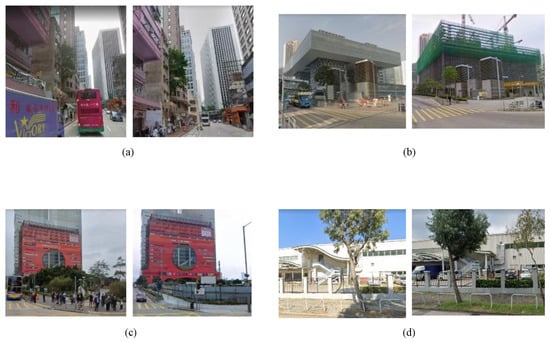
Figure 1.
Existing problems of street-level image based geo-localization. Images are from our street-level image dataset. (a) shows occlusion of traffic flow in a block of Hong Kong. (b) Background occlusions as people flow and trees are hardly ignored in positioning of urban streetscapes. (c) New construction and renovation of urban buildings will have an impact on recognition and precise positioning of target objects. (d) Impact of photo shooting direction in IBL—it may cause mutual occlusion and morphological differences.
The engineering application of IBL in metropolitan scenarios must consider issues of processing massive data such as compression, storage, retrieval optimization, etc. Information of street-level images in main roads and branch roads, prosperous areas and remote suburbs, etc., has different characteristics. Therefore, solution of IBL should be robust to diversification and volume of data.
Different methods have different emphasis. Image retrieval is a feasible solution to meet IBL challenge. It focuses on selecting representative features to characterize the query image and retrieving correct reference image as much as possible. All reference images in the database have real GNSS coordinates. After matching process, the shooting position of query image can be estimated by the GNSS-tags of its correctly matched reference image. There are two key points worth noting in selecting image retrieval method to meet the challenge of IBL.
One key points of tackling IBL task through image retrieval is to learn the discriminative feature. Feature learning in urban scenes must first suppress the influence of meaningless things in distinguishing images. To distinguishing urban scenes, relatively static landmarks own decisive significance, such as buildings. Other things that are changeable and fluid are meaningless. Therefore, we focus on the features that falling on the building and use them as the core of feature design.
Features can be divided into local feature and global feature based on representational content. Local features can be divided into hand-crafted and CNN-based according to their production process. Global features include aggregated features which based on CNN.
Research on hand-crafted features, which focus on local details, provide solutions to IBL problem [17,18]. Complex urban scenes will bring great interference, like people flow, billboard, cars, etc., to the image matching process based on these local features. But these methods are not accurate or robust enough with multiobjects. Embedding methods [19,20,21,22] proposed later are focus on aggregating discrete local features to generate more identifiable image features. Usually, the aggregated long feature vector has a high dimension, which affects its storage and loading. This property makes them hard to generalize to real scene image retrieval applications. In the age of deep learning, global feature descriptor extracted by CNN made progress in image matching [9,23,24,25]. Global features perform well in specific object recognition and classification tasks. However, a certain region containing specific object in one image may play a key discriminative role in image matching. Other parts of the image, which containing other nonspecific objects, will be considered as noise in image matching.
We synthesized characteristics of the features analyzed above: there is still much potential for global features in patch-level matching. Local features are fit to capture details, but massive storage amount and meaningless information still need to note. Hence, we will promote expression of feature in patch-level matching and make storage optimization.
Another key point of image retrieval is to refine the matching form between query image and database image with reference. A typical IBL task can be divided into two stage: one is image recognition, the other is visual localization. The later also called geometric verification. Geometric verification stage has problems such as too many sample points in modeling, which may lead to no optimal solution or excessive solution time. RANSAC [26] is widely used [27] in the geometric verification stage. So, we will pay more attention to the quantity and quality of feature points used for modeling in RANSAC.
This paper mainly contributes these: (1) we propose Building-Aware Feature as we comprehensively considered the discriminativeness of the building in urban IBL task and the patch-level matching ability that the feature should have. BAF is the product of a trained classifier, which classifies the attention features extracted by CNN, thereby lessening some irrelevant features that fall on nonbuildings. (2) We proposed stage of geometric verification by contribute a patch-region retrieval (PRR) algorithm. PRR is to perform visual localization, also called geometric verification stage of image retrieval, through feature points in patch-regional query image. A query image is divided into several patches. Select the best retrieval ranking to represent the whole query image among these query results of patch-regions. Our experiments based on a metropolitan-scale dataset we collected show that BAF not only selectively retain related feature and compress the storage of index, but also improve accuracy of image retrieval; PRR has improved the retrieval effect of our features BAF and other features in our experiments.
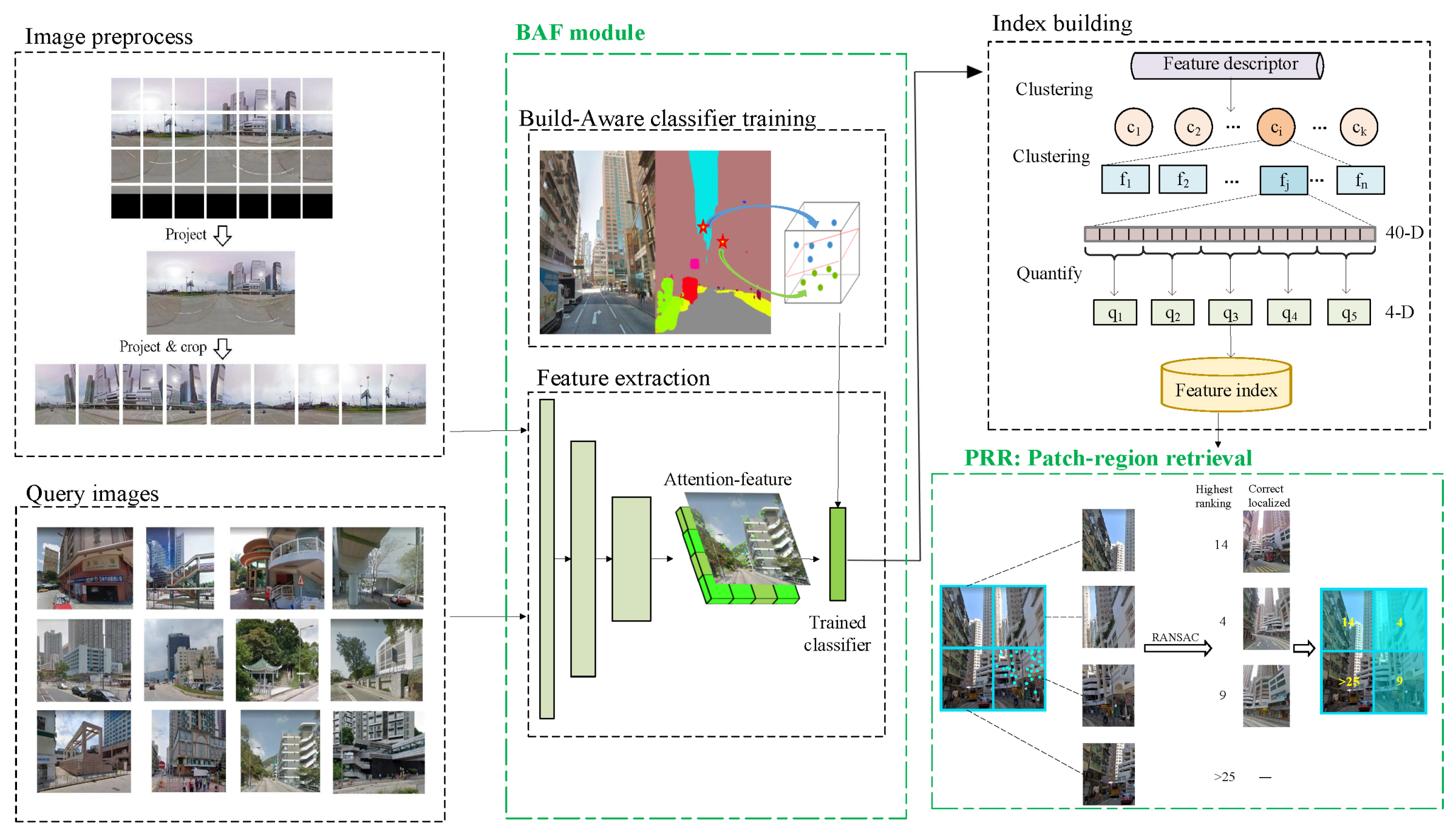
The complete framework of this paper is shown in Figure 2.
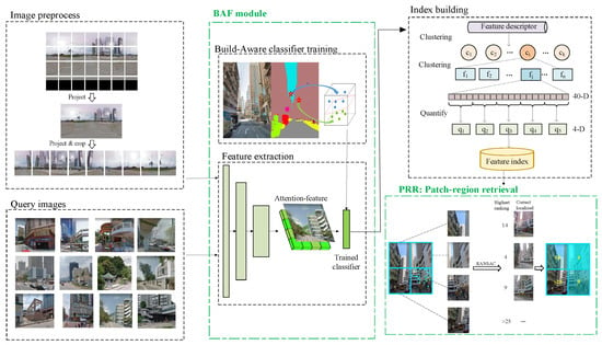
Figure 2.
Technology roadmap of our whole framework.
2. Materials and Methods
2.1. Related Work
Instance-level image retrieval is widely used in the practical situation and related research is also concerned [27,28]. Instance-level image retrieval needs to learn the differences between categories in a large amount of category information [29]. According to the characteristics of feature descriptors, existing researches can be divided into the following methods: local feature, aggregation of local feature, global feature, and combination of global feature and local feature.
Hand-crafted local features [17,30] usually use the visual vocabulary of BoW [31] to do retrieval. It can effectively complete small-scale single object retrieval. Studies later put forward emphasize more on precise quantification of local features [18,32]. Features focusing on local clue have their detection mechanism of key points, which limits their performance under occlusion, clutter and illumination in complex scenes. Accuracy and robustness of hand-crafted local feature in matching are difficult to maintain in such a kind of situation. Local features based on CNN in face recognition like [30], improves the computing cost of hand-crafted feature like SIFT [17] or SURF [18]. However, these methods have not been specially optimized for large-scale street-level image retrieval problems. DeLF put forward a complete large-scale retrieval framework, which is closely related to our goal. But the time spent in once retrieval and memory requirement are hard for it to solve.
The prevalence of deep learning brought many outstanding aggregation methods and global features. Aggregation method is to establish connected vectors [21,22,29] based on discrete local feature vectors, or to derive the symbolic functions [20]. This needs to consider the problems caused by high-dimensionality of the connected feature vectors, which affects the storage and loading of it. This property makes them hard to generalize to real scene image retrieval applications.
The development of global features is mainly the improvement of loss function [9,25] and pooling layer [22,23]. Global features perform well in specific object recognition and classification tasks. However, a certain region containing specific object in one image may play a key discriminative role in image matching. Other parts of the image, which containing other non-specific objects, are considered as noise in image matching. The limit of global features in image retrieval is the imperfection of patch-level matching ability [27,28,31]. To improve, some researchers [31,33,34] formed a new matching kernel on patch-region of one image’s subregion. Or use the same CNN to train local features and global features [35].
Given the characteristics of the above-mentioned features, our work will adopt a method of local feature, which is based on CNN. Using a trained classifier, the feature points of buildings that are important for street-level retrieval can be retained with a trained classifier, and the feature points that fall on non-buildings are filtered out. SVM is a classic classification algorithm [36], which also performs well on nonlinear-separable situation [37]. We use this algorithm for training our classifier.
In field of computer vision, RANSAC is usually used to solve problems of matching points of a pair of cameras and the calculation of the basic matrix [38]. RANSAC always appears in the re-rank stage of image retrieval [27], which is also named the geometric verification stage. The factors that affect the speed of RANSAC are mainly the choice of the established model and the number of modeling points. This paper will start with optimizing the number of modeling points and improving the quality of modeling points to achieve rapid localization of street-level images.
These image retrieval methods [8,20,27,29,34,35] are performed on these standard retrieval datasets [20,39,40]. Considered scales of these datasets are small and have no GNSS coordinates. These defects are difficult to overcome, so these retrieval methods are difficult to generalize. Large-scale datasets [27,31] can provide large number of categories, which enables CNN to learn discriminative features. They are suitable for solving tasks like recognition, object detection and geographical position classification tasks, not IBL task. Because they overlook IBL, tasks based on street-level images have the nature of weak category labels. Street-level dataset that has real position information is suitable for IBL, which overs continuous and dense road network of city. The dataset used in [20,41] is to solve the problem of scene image recognition and retrieval in night, which has a certain specificity. The dataset used in [8] considered multiple perspectives of one position.
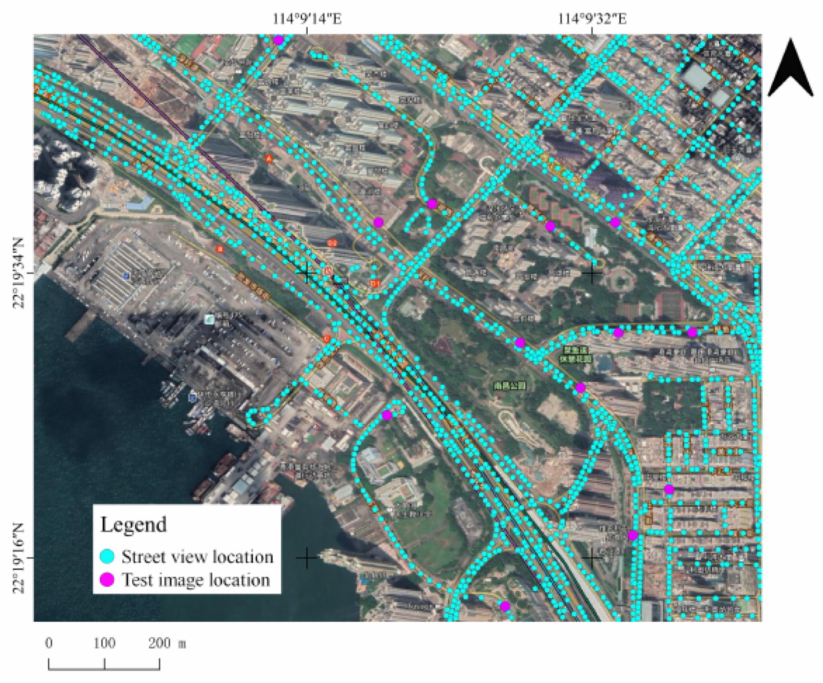
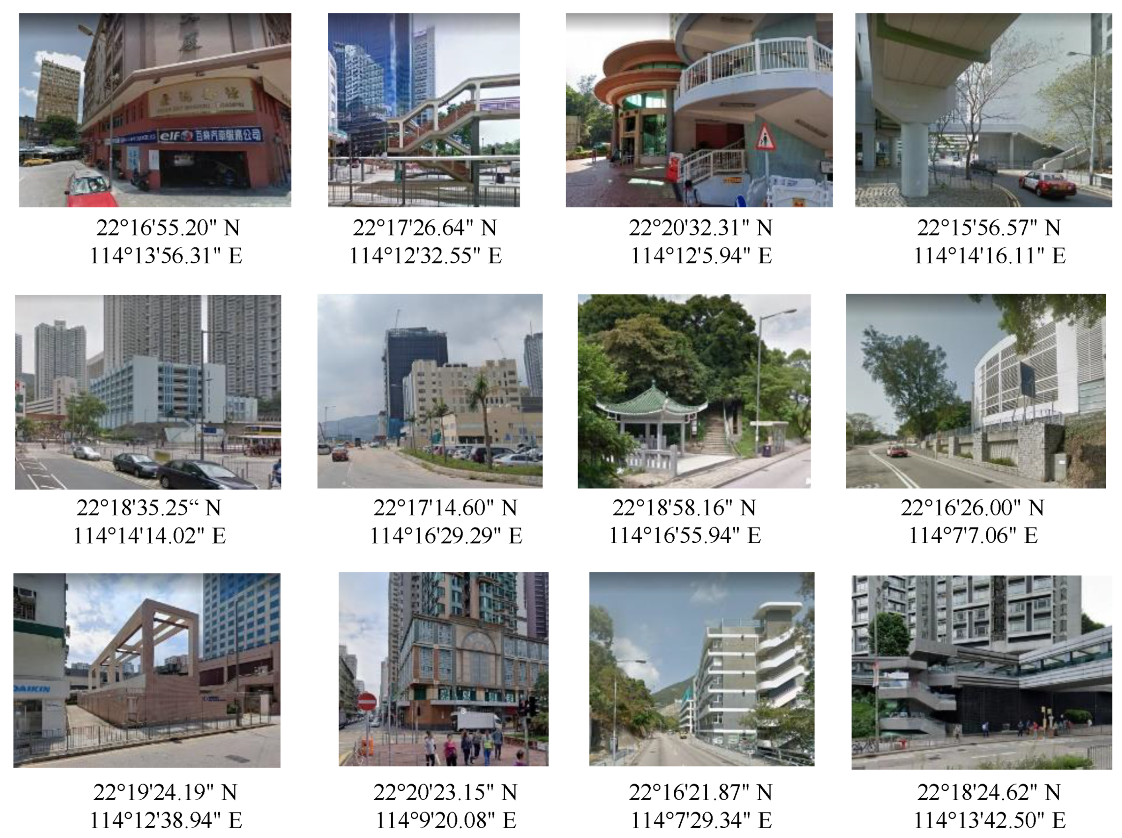
We collected a street-level image dataset shown in Figure 3 that covers almost all of Hong Kong and has 337,323 points, a total of 9,445,044 images. Each point has a GNSS coordinate. This dataset consists of several distinct scenes of urban, suburban, and rural areas. The test dataset in Figure 4 consisted of 337 images collected from news images, online images, and field shots. Our dataset is suitable for solving the IBL problem on a city scale. In addition, GNSS coordinates, as a class label, is a kind of weak label information. The characteristics of our data determine that it is difficult to use them to train the CNN network to converge. Therefore, methods of global feature have imperfections in tackling IBL task with street-level image.

Figure 3.
Distribution of part of our Hong Kong street-level image dataset and part of our test data set on satellite maps.
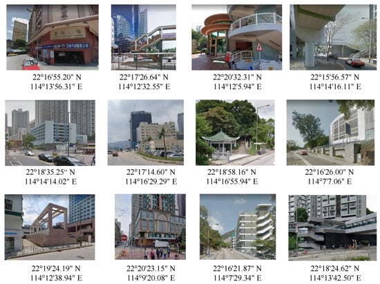
Figure 4.
Part of our test dataset: each test image has latitude and longitude coordinates.
2.2. Our Method
In this section, we will focus on the principles and related formulas of BAF, as well as the details of BAF-based PRR method.
2.2.1. Building-Aware Feature
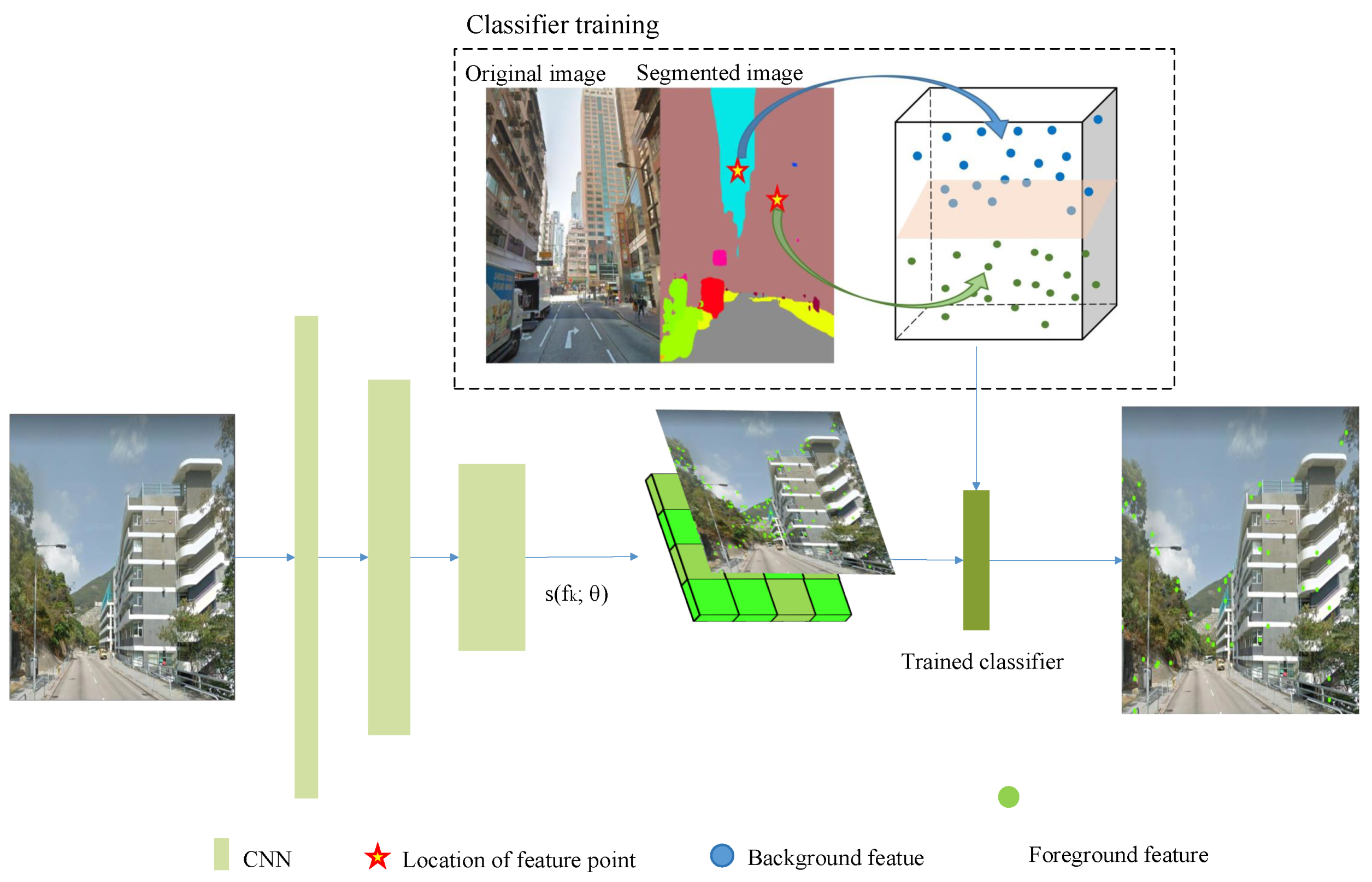
Figure 5 shows the entire processing flow of BAF. The principle of BAF mainly includes two parts: deep feature extraction and building-aware classifier training. The former learns the use of attention module and the selection mechanism of key points in [27]. The building-aware classifier is trained based on the features annotated by PSPNet [42] and is used to classify the extracted deep dense local features.
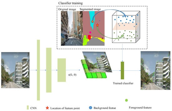
Figure 5.
Extraction architecture of BAF: green bright spots is feature descriptors. After classification of building-aware classifier, number of descriptors falling on sky, woodland, etc., decreased significantly.
Building plays an irreplaceable role in recognition and matching of street-level images. Relatively speaking, static objects or dynamic objects such as trees, vehicles, people, etc., in complex scenes of street-level images have unstable or even little meaning for recognition and matching of street-level images. Feature points falling on these things can cause mismatches. BAF is proposed in response to this problem, and its main contribution is to lessen irrelevant feature points.
Feature Extraction
Street-level images are fed into the Resnet50 network [43], which was pretrained on ImageNet. The discriminant ability of local detail expression can be improved by fine-tuning. Here, we use the network layer before the convolution block of ResNet50 as our fully convolutional network (FCN). To deal with scale change, we use the FCN mentioned above to construct an image pyramid and apply FCN for each level. The output features of FCN, which are denoted by .
Then, connect the attention function to the output of of ResNet50 to obtain the relevant score of local features. The features with attention scores are described as:
The output is the feature vector with attention score. M is the top M features ranked according to the attention scores. denotes parameters of function. Attention function is strictly limited to be non-negative. As a soft-plus [44] activation function on the top of the attention module. This method first generates embedding on the entire input image, and then the softmax-based classifier is connected.
Use the pixel in the center of the receptive field as the position of one feature. According to nonmaximum suppression [45], retain the feature points with the highest attention score in the same pixel of image. Use PCA [46] to reduce the dimensionality of features at each level of image pyramid. The feature vector after dimensionality reduction is expressed as . is the dimension of feature vector after dimensionality reduction. Dimensionality reduction achieves the proper balance between compactness and discriminability.
Organize all the feature points at each pyramid level after dimensionality reduction into a feature description of an image. By using image pyramids, we can obtain features that describe areas of the image of different scales. In addition, we have learned advanced semantic information of the feature map through attention encoding.
Building-Aware Module
Building-aware module introduce the transform of the extracted dense features to building-aware features. As mentioned before, there are blocks in urban street-level images like people, vehicles, billboards, and trees. These objects bring noise interference to our image feature matching. Therefore, we will focus on the decrease of irrelevant noise feature points to improve the quality of feature points. Applying a classifier to classify and filter feature points is a direct and effective way. Hence, the goal of this section is to introduce process of train a fit classifier to compress redundant features.
Before training the classifier, we need to classify the feature points.
Pyramid scene parsing network (PSPNet) [42] with a pyramid parsing module is an improvement of FCN. It combines local and global clues, making it more reliable to predict the difficult scenery context features. PSPNet introduces more contextual information to complete the segmentation through the following operations: (1) increase the receptive field, including dilated convolution and global average pooling; (2) confuse feature maps in different levels generated by pyramid pooling. Given PSPNet’s excellent performance in both grasping global features and capturing local features, we use the segmentation results of PSPNet to label our feature points.
The labeling rule is: the class of the feature in a pixel is the segmented class of this pixel. The labeled feature is described as follows:
P is network of PSPNet. represents the labeled class that belongs through PSPNet. In our work, is included in five classes: buildings, trees, roads, sky, and billboards. These classes are segmented by PSPNet according to our street-level images.
After labeling, the dataset of features can be described as .
Solving the Lagrange objective function is key to train the SVM classifier to find a hyperplane in labeled features.
Considering the dimension of the sample data and the linear indivisibility of the dataset, we use radial basis function (RBF) as the kernel function to map D to the linearly separable high-dimensional space. In the high-dimensional space, the formula of hyperplane describes as follows:
where is the normal vector, which determines the direction of the hyperplane. b is the displacement term, which determines the distance between the hyperplane and origin of coordinate system. In general, the hyperplane is represented by , because it can be determined by normal vector and displacement b.
In this paper, t is the classification threshold, and labels of other classes are smaller than t. Therefore, the expression of positive and negative samples in the hyperplane formula is as follows:
The partition hyperplane in the middle of positive and negative samples is the most effective hyperplane in sample learning. This requires us to find the maximum interval between positive and negative samples in the sample space. Among the training sample points, the nearest to the hyperplane makes the equal sign of the above Formula (3) true, and these training samples are called support vectors. In the classical derivation process [36,37,47], the interval between positive and negative samples is taken as . In this paper, because the label value of each category is greater than or equal to 0, the interval between positive and negative samples is shifted to . So, the sum of the distances from the two positive and negative support vectors to the hyperplane is expressed as follows:
After quantifying the distance expression, we transform the model training into a convex quadratic programming problem. Considering that the Lagrange function has strong duality, we simplify the training target from the expression of entire Lagrange function to the expression as follows:
The Lagrange multiplier . The KKT condition is:
In our work, the class c of a feature is determined by the following formula:
If is greater than the threshold t, will be labeled which refers to a building feature. If is less than t, is judged as a nonbuilding feature and labeled .
The vector classified by the classifier is expressed as . The feature dataset is described as .
We call features that fall on buildings as building features, and features that fall on nonbuildings as nonbuilding features. The purpose of our trained classifier is to lessen redundant background features. Considering that background features may be useful for image matching to a certain extent, we make the best classification hyperplane a bit closer to the negative samples. After getting the class information of all the features, we start to build the index.
2.2.2. Image Retrieval with Building-Aware Feature
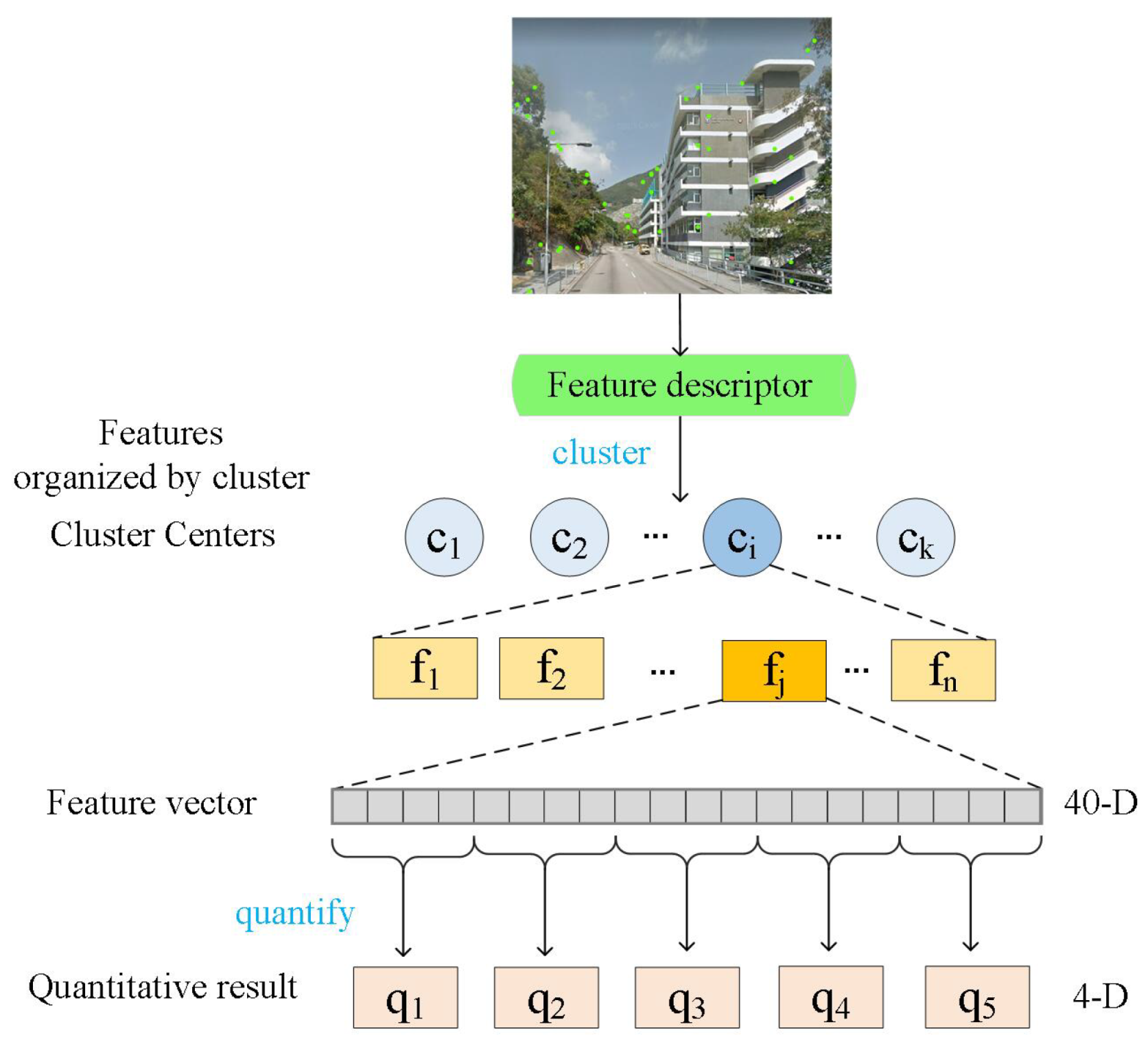
In this section, we will introduce the procedure of image retrieval with BAF. The procedure mainly includes establishment of index, as shown in Figure 6, and retrieval process. Firstly, we choose K-means clustering and product quantization (PQ) [48] to build index. Then, we use inverted index [49] and nearest neighbor search algorithm to complete the first rough matching of features. Finally, implement our patch-region retrieval algorithm based on RANSAC [26] to rerank the retrieval results of the first matching.

Figure 6.
Inverted index and product quantization schematic diagram.
Establish Index
We use the classified features to train the initial cluster centers. Define the initial number of cluster centers as K. Describe the loss function as follows:
After training the initial cluster centers, we need to insert features into their corresponding cluster centers according to the nearest Euclidean distance.
In each cluster center, we perform product quantization on the inserted features: divide each 40-dimensional feature into 10 segments of 4-dimensional features. Then, we apply k-means clustering again in each cluster center. We use the numbering of cluster center after the second clustering to encode the feature.
Hierarchical Navigable Small World (HNSW) [50] is an ANN search algorithm based on multilayer graph, and its accuracy was largely improved. So, we choose it as the method of the first rough retrieval.
Implement Patch-Region Retrieval
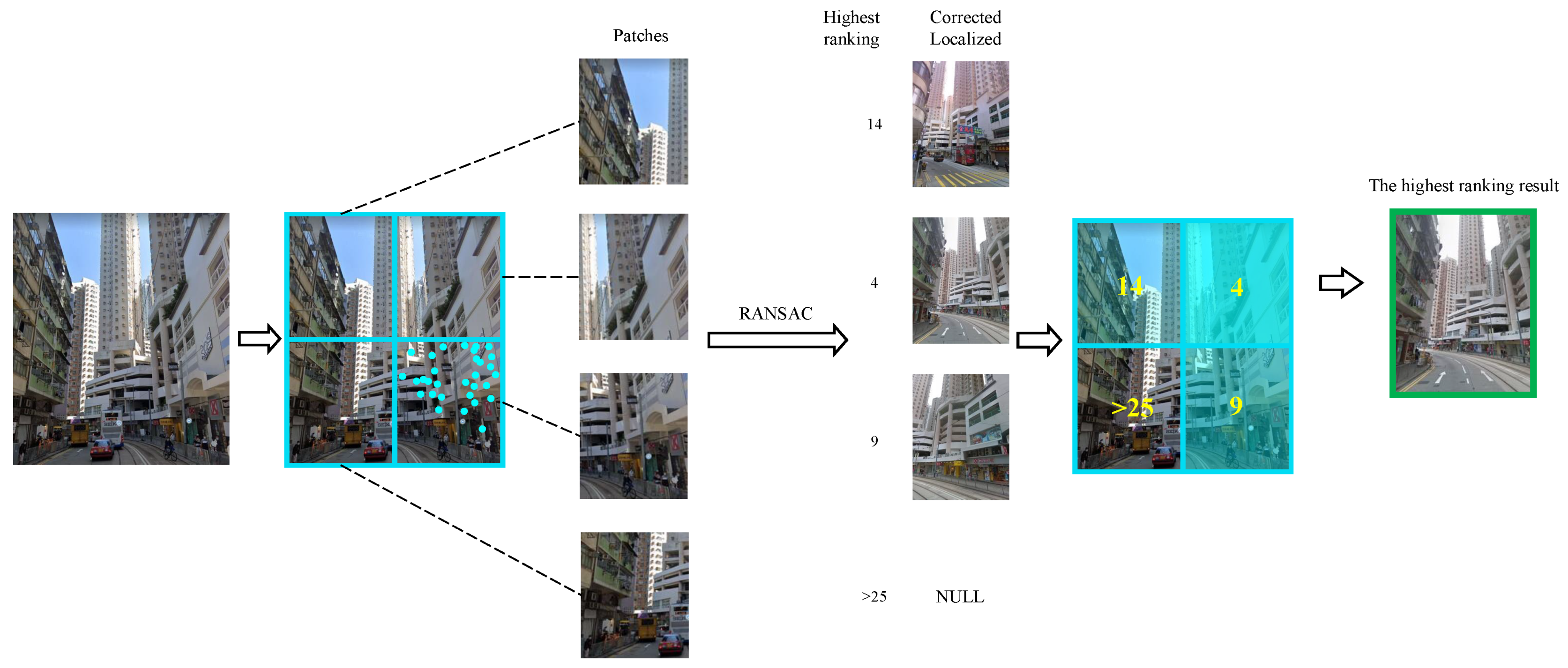
We drew the whole process of PRR in Figure 7. In the geomety verification stage of retrieval, the model used in RANSAC is as the affine transformation model. The affine transformation is as follows:
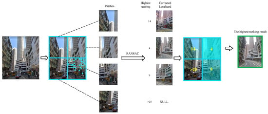
Figure 7.
Schematic diagram of patch-region retrieval method. Take 4 partitions as an example: divide query image into 4 patch regions with 2 rows and 2 columns. Perform geometric verification on these regions in turn. Localization result, which can be correctly positioned and with the highest ranking in these areas, is used as positioning result of this query image.
p is the coordinate matrix of sampling point. n is the coordinate dimension. i is the minimum number of sampling point set in RANSAC to build the model. A is the affine transformation matrix, and b is the translation vector. According to the solution of RANSAC, we randomly select sampling points to build the model. Then, we can calculate the affine transformation matrix A. Under the maximum number of iterations, we take the model which has the largest number of inliers that can meet the residual threshold condition as the solution. A is an invertible matrix. In the actual solution process, we will convert A into augmented matrix and augmented vector for calculation.
Before model solving process of RANSAC, we divide the query image into grid patches. The format of the divide is j rows and j columns. Then, we perform the matching process of each patch image in turn.
The formula for patch-region retrieval is described as follows:
is the patch region of query image that be input in the patch-region retrieval framework. expresses the procedure of feature expression and patch-region retrieval. The ranking of the highest query result is used as the matching result of this image.
3. Experiments
3.1. Dataset
Street-level images are the basis of image-based localization researches and were used in a number of methods [8,9,20,41]. We collect the street-level image dataset used in our experiment from Google Maps. This dataset covers most areas of Hong Kong including Hong Kong Island, Tseung Kwan O and Kowloon Bay, and contains almost all road-nets. Each sampling point provides panoramic data with latitude and longitude coordinate information. Panorama can be projected to certain angle, providing multiperspective street-level images [8,9], and catering to randomness of query images.
The street-level dataset we collected contains 337,323 sampling points as shown in Table 1. After the sparse processing, we have 87,691 sampling points. The road network covered by the sampling points includes the following scenarios: urban blocks, suburban roads and rural roads. Sampling points evenly distribute in these scenarios. Each sampling point is associated with GNSS coordinates. The image data of each sampling point consists of 28 images in 4 rows and 7 columns, which projected from a panorama. Due to the annular perspective, images in one sampling point have complex street view, buildings, people, vehicles, trees, roads, billboards, telegraph poles, etc. In summary, there are three concerns in the retrieval and location of our dataset: (1) how to index the huge amount of data in an orderly way; (2) how to extract high-quality features to effectively describe complex scenes; and (3) how to distinguish multiple scenes under the same GNSS-tag.

Table 1.
Information of our street-level dataset before and after sparsing.
As for test dataset, we collect 337 query images from web page of hot news, Google street-level map, and field shooting. Each query image has a pair of latitude and longitude coordinates of the location.
3.2. Experimental Equipment and Environment
To facilitate readers to reproduce our method, we list the hardware equipment and software environment used in this paper in detail in Table 2 and Table 3.

Table 2.
Information of hardware.

Table 3.
Information of software.
3.3. Data Preprocessing
This section describes the preprocessing of images of sampling points before feature extraction. It consists of two parts: sparse sampling point and adjust the images. The sparse work is to eliminate redundant image data due to sampling spacing. Image adjustment is to carry out three tasks on the image data included in each sampling point: (1) stitch the grid-like image data into panorama; (2) back project panorama; (3) and crop the projected data as database image to extract features.
3.3.1. Make Sampling Points Sparse
Considering the following two points, we need to make our street-level sampling point sparse: (1) there are dense buildings and interlaced streets in urban areas, so street-level image obtained from adjacent collection points may have certain similarities. (2) When the scale of street-level image data getting large, calculation cost and processing speed will become a problem that can not be ignored.
We downloaded road network data covering the experimental area from “OpenStreetMap” website. Perform the following operations on the road network data: firstly, the road network data is discretized into scatter point data.
Then GNSS coordinates of each point is used to insert the collected data points into the scattered road network. In this step we use K-D tree structure to insert points that match the sampling point and its corresponding road. Because K-D tree uses binary to divide data space, which is easier to be realized in memory [51].
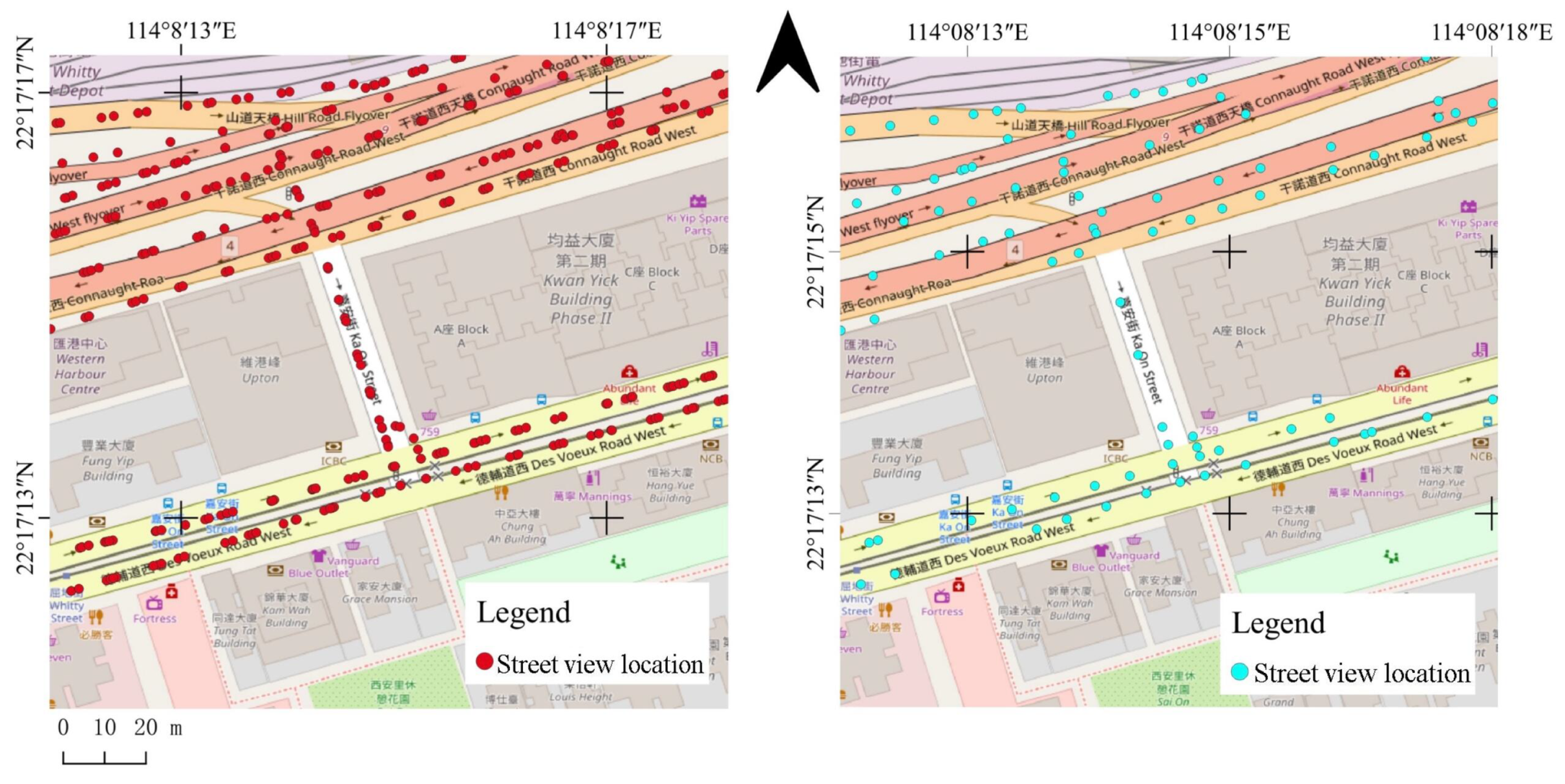
The sparse rule is that on the same road, the distance between two sampling points shall not exceed 10 meters. If the distance exceeds 10 meters, delete the point to be inserted. For points meeting the sparse insertion rule, we use R-tree to store, because R-tree [52] is balanced and has a variety of optimization strategies, which is more suitable for changing data storage.
We can visually see the reduction of sampling points in Figure 8, and the comparison of memory requirement in Table 1 before and after sparing process. Our sparse work effectively lessen the data volume of megacity Hong Kong by 100%·(1 − 71 G/273 G) = 74%. The follow-up work of IBL’s application will benefit from the reduction in data volume.
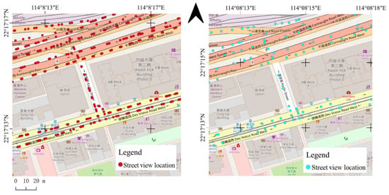
Figure 8.
Effect of sparsing process performed on street-level sampling points: left is before process; right is after process. Streetview sampling points become sparser.
3.3.2. Projection and Cropping
Considering the state of the street-level image data we collected, we preprocessed the images projected from the plan to the spherical image, and then to the plan. We will elaborate the process as follows:
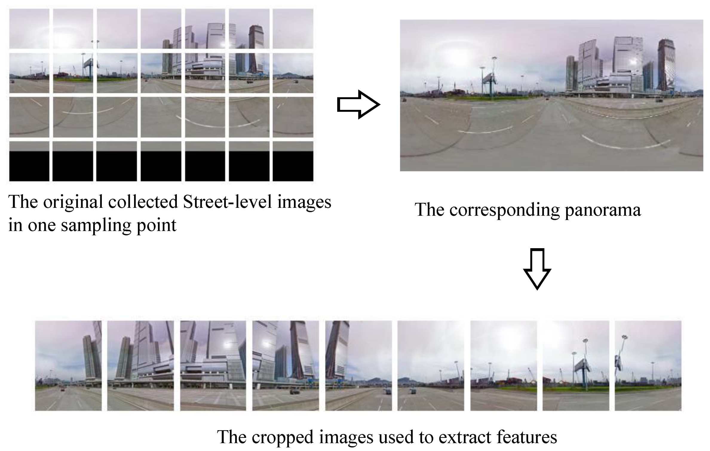
The grid-like images contained within a point, including 28 images of 4 rows and 7 columns, are all plans. To extract effective features for each point, the images need to be joined together and projected as one spherical image, which is a panorama.
There is a large geometric deformation at the edge of panorama. Moreover, the panorama which has a circular view includes complex scenes, so it is not suitable for feature extraction as a database image. It is necessary for panorama to be projected and cropped to plans, which with the right angle of view for query.
To reduce the visual distance between the real street view image and the panorama, we use the spherical projection algorithm [53] in this paper to project the equirectangular panorama into the local plane without distortion. The conversion formula is as follows:
is the transformation function from Euler angle to rotation matrix, and denotes Euler angle. G represents imaging plane, and G is transformed by function to obtain imaging plane in Euler angle direction.
X and Y denote the abscissa and ordinate of the pixel on the equirectangular panorama, and (x, y, z) represent the 3-D coordinates of the pixel in the imaging plane.
We use a method to generate horizontal perspective plan, which is based on the Iso-rectangular projection of panorama. Standard camera has an angle of field of view (FOV) between 40° and 45°. Taking into account the image perspectives in the test dataset we collected, we set the horizontal perspective of the panorama projection as 40°. Then 9 subimages of panorama are obtained.
The processing flow of this step is shown in Figure 9.
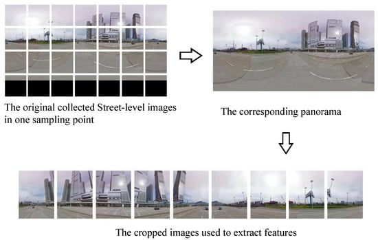
Figure 9.
Graphical description of preprocess, take one sampling point as an example: firstly, grid-like images are collected for spherical projection, and then stitched it into a panorama. Street-level images of each sampling point consists of 4 rows and 7 columns. Panorama is then projected into a plan and cropped into 9 subimages.
3.4. Extraction of Building-Aware Feature
3.4.1. Extract Original Deep Feature
We use the backbone to extract BAF from 9 images at each point. The backbone is the output of of ResNet50 and is connected with the attention module trained by [27] and the classifier trained by us. Before filtered by the classifier, the number of feature descriptors in each image is no more than 1000. Each descriptor is a 40-dimensional vector. The descriptors of each point occupy less than 0.69 MB of memory. The extraction results of these 9 images are classified and saved according to GNSS coordinates of each point.
3.4.2. Label Features for Training Classifier
PSPNet [42] gives a reliable direction for pixel-level prediction tasks, as both local and global clues are considered. The backbone of PSPNet is also based on ResNet50, which is consistent with the extracted descriptors. In the experiment [42], PSPNet shows excellent segmentation performance in distinguishing objects in Cityscapes dataset [54]. So, we chose segmentation results of PSPNet as the standard to annotate our street-level image data.
We use PSPNet to segment 50,139 cropped images randomly selected from our street-level dataset to provide object-level annotation for each street-level image for training SVM classifier. We selected buildings, trees, billboards, people, and other 5 classes from the segmentation results of PSPNet. The building feature is the core part of our retrieval task. We labeled the image descriptors falling in the segmented region by class information of the region.
After segmentation, 826,968 feature descriptors were obtained. A total of 50,000 descriptors were randomly selected for training classifier, and 165,364 descriptors were used for testing.
3.4.3. Train Classifier
Classic SVM algorithm is chosen to classify nonlinear data by kernel function [37], as its classification features can be explained and it has fault tolerance ability for outliers. We use radial image kernel function (Gaussian kernel) to transform features’ dimensions. The transformation is from high to low dimension. It can make features linearly separable in high-dimensional space. To make the classifier more sensitive to buildings, we chose a one-versus-one (OVO) approach to train the SVM classifier. Five-fold cross validation is used to evaluate the accuracy of the model. The training hyperparameters of the SVM classifier are shown in Table 4. ’Classifier training’ module on top of Figure 5 is a schematic diagram of the classifier training.

Table 4.
Setting parameters of training SVM classifier.
The training information of the building-aware classifier are shown in Table 5. Specifically, Recall and Precision in Table 5 refer to buildings relative to non-buildings.

Table 5.
Training information of Buiding-Aware classifier.
Using the SVM model we trained, most building features were retained and most nonbuilding features were filtered out. Compression rate of features that we can achieve is 25%.
3.4.4. Filter Feature Descriptor
The accurate identification of buildings is one of the most important factors to determine the success of urban street-level localization. Large scale dataset has a large number of redundant data. To complete the IBL task efficiently, it is the starting point how to distinguish between nonbuilding features and preserve building feature. The significance of the training classifier lies in keeping the feature points falling on building objects as much as possible while deleting the noises.
We input the descriptors into the classifier. This step is after attention function and dimensionality reduction, and each descriptor is 40-D at this time. Trained SVM model function value less than 0 is regarded as a negative sample, and this part of descriptors is filtered. Considering that some background features may have a positive effect on image matching, we set two filter thresholds: −0.5 and 0. The two experimental results will be detailed in Section 5.
3.5. Image Retrieval
To meet the challenge of street-level image features in metropolitan-scale, we need to take effective quantification measures for the feature points; in the retrieval reordering stage based on geometric verification, we need to improve the impact of meaningful dense points for retrieval result.
3.5.1. Initial Detection
Input the query image into the network to extract building-aware feature. We connect the attention function after the output of conv4_x of ResNet50, which is to obtain relevant attention scores of feature points. For each image, we select the first 1000 feature points with the highest score to represent this image.
Then, calculate the similarity between the query image and the image in the database. Similarity is measured by the Euclidean distance between feature points.
With the help of index, we find the images in database with the highest similarity to the query image. Similarity is measured by the Euclidean distance between vectors. We use top500 matching images for reranking.
3.5.2. Build Index
Faced with tens of millions of descriptors, how to store and manage them in an orderly way is a challenge. We use PQ to quantify descriptors, thereby reducing the storage required for index. We also use inverted index and ANN search to speed up the process.
Firstly, we use all the classified descriptors to train the initial cluster centers, which are also 40-dimensional vectors. The reasonable number of cluster centers is selected 216. Then, all features are inserted into the nearest cluster center according to the nearest asymmetric distance. After the first clustering, we segment the feature vectors in large cluster center. Each 40D descriptor will be divided into 10 segments of 4D short vectors. In each large clustering center, secondary clustering is carried out for all the segmented vectors, and a 256D codebook is compiled. Each small cluster center corresponds to an integer number. The distance between the codebooks is calculated in advance and stored in metadata. In this way, a 40D floating descriptor can be transformed into a 10-D integer descriptor. This conversion greatly speeds up the query process.
3.5.3. Retrieval Reranking
The first retrieval process is to compare the Euclidean distance twice between clustering centers, so as to find the most similar descriptor and get the matching result. Each time we finish retrieval with ANN search. The second retrieval process is to use RANSAC framework to complete the reranking of retrieval results, also known as geometric verification. We establish an affine model in RANSAC framework for image matching.
RANSAC uses an iterative approach to estimate the parameters of the mathematical model from a set of observed data. The algorithm assumes that the data contains correct data and abnormal data. Correct data are recorded as inliers, while abnormal data are recorded as outliers. In this work, the matching degree of two images is represented by the number of inliers. The core idea of the algorithm is a hypothesis. Hypothetical means that assuming that the selected sample data are all correct data, and then use these correct data to fit a model, calculate the deviation of other points to the model, and score the model.
After the first search, we obtained quite a number of resulting images. We set the number of resulting images that participated in the geometric validation process to 250. The minimum sampling set for the affine model is set to 3. The maximum number of iterations is set to 1000.
Our patch-region algorithm is implemented here: firstly, the query image is divided into 2 rows and 2 columns or 3 rows and 3 columns, and then geometric verification is performed on the descriptors of each subimage in turn. Select the best matching result as the matching result of the whole picture.
4. Discussion
In this section, we will discuss and analyze experimental results. Also, in patch-region retrieval-related experiments, the image is divided into 2 rows and 2 columns, which is represented by 4 in the legend of table, and the picture is divided into 3 rows and 3 columns, which is represented by 9 in the legend of table. BAF and BAF2 represent classifier thresholds of −0.5 and 0, respectively. For example, BAF2_9 means that when the classifier threshold is 0, 33 partitions are used for geometric verification with patch-region retrieval experiments. The recalls of all experiments are shown in Table 6.

Table 6.
Recalls of experimental methods.
4.1. Comparison of Time Cost
Time cost is an important indicator to measure localization method. The localization time includes retrieval time and judgment time. We have counted positioning time of different features in Table 7. Retrieval process of each query image includes feature matching and geometric verification. Besides, the localization time also includes judgment time, which is calculate the real distance between the query image and the retrieval list. Only if the distance is less than threshold 25 m, we think it is the correct localization result. As shown in Table 7, localization time is the average time of 50 test images.

Table 7.
Time cost of different features.
In our experiment, BAF demonstrates its superiority in time cost. Time cost in stage of matching features from index is low. Matching time of different features is shown in the Table 7. Time cost of BAF and BAF2 is shorter than that of DeLF. But the overall situation is similar, the matching time using BAF is shortened by 0.14 s per image. The geometric verification stage is time-consuming. Because it is necessary to solve the affine model. In general, to locate an image, using BAF is 0.2 s faster than using DeLF.
4.2. Effectiveness of BAF
4.2.1. Reduce Storage
As shown in Table 8, BAF significantly reduced 18.9% more storage space than DeLF. Moreover, BAF2 reduced 29.7%. These numbers fully prove that our feature is more concise than the mainstream feature method. In metropolitan-scale engineering applications, our features are more competitive. We can see indexes of ORB and BA-ORB require more storage space. From this point on, features based on deep learning are better than hand-crafted features.

Table 8.
Metadata of different features and memory size decrease after building-aware classifier.
4.2.2. Improve Localization Effect
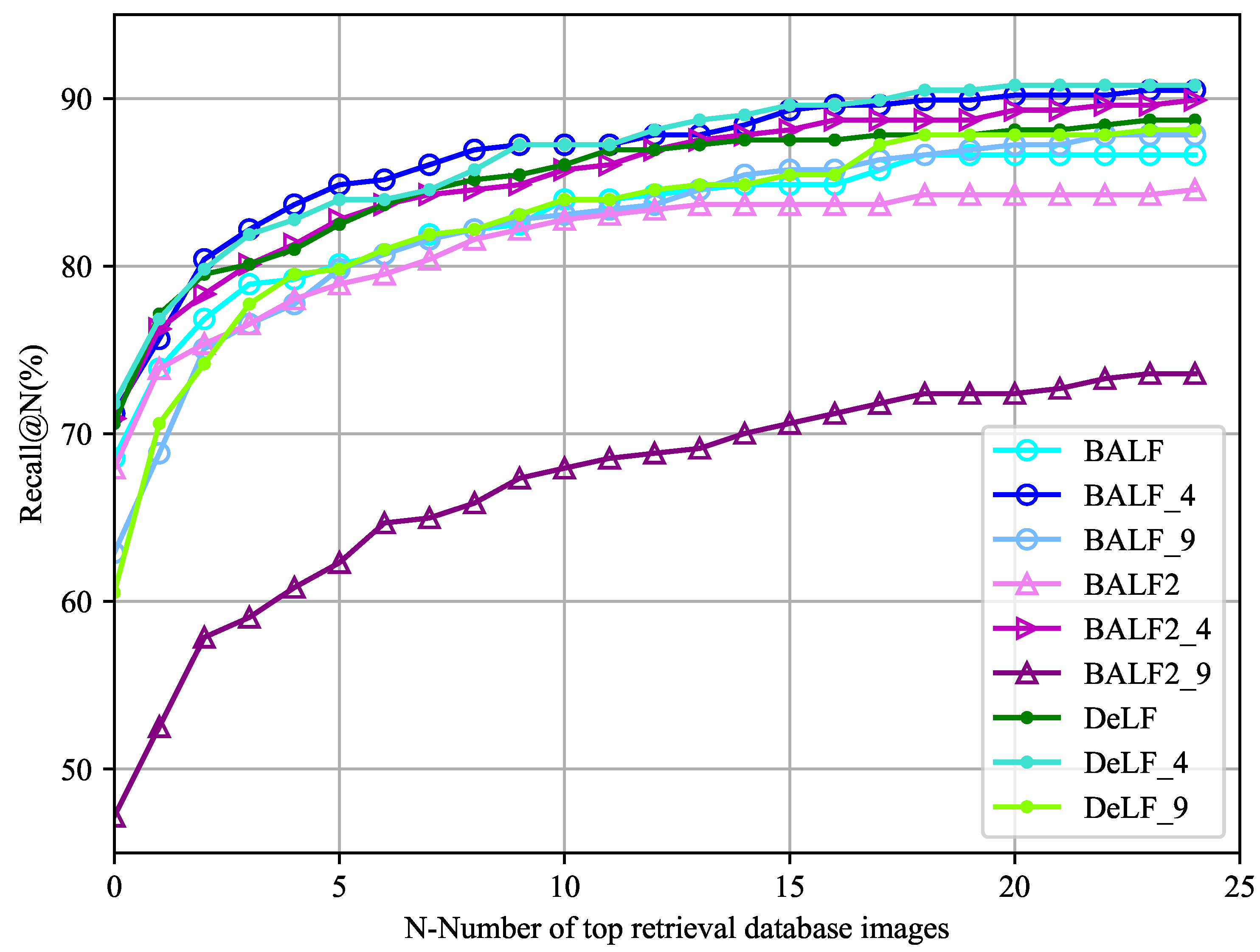
The overall trends of recalls of different experiments are shown in the Figure 10 and Figure 11. Figure 10 shows the top 4 best localization experiments.
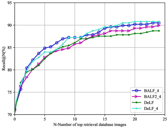
Figure 10.
Positioning effect of best 4 experiments measuring by Recall@N. BAF_4 showed best performance in front position, and DeLF_4 showed best performance in back position.
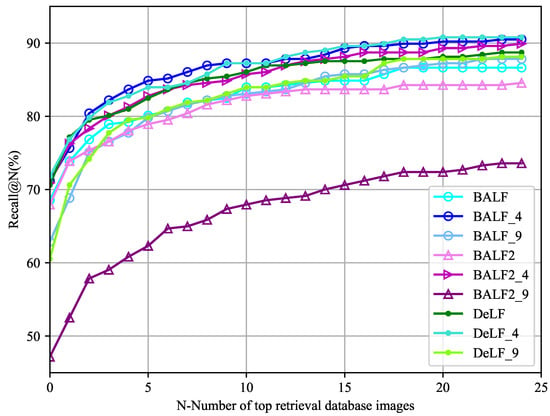
Figure 11.
Positioning effect of all experiments measuring ny Recall@N. Both BAF and patch-region retrieval show good performance.
On the test dataset we collected, BAF_4 achieved the highest accuracy between Recall@3 and Recall@12. According to table, other Recall@Ns are ahead of DeLF except Recall@2, leading the highest percentage at Recall@5 by 2.67%. BAF2_4 performed better than DeLF after Recall@13, leading a maximum of 1.19 points. But percentages between Recall@8 and Recall@12 are slightly lower than DeLF, with an average of no more than 0.55 points.
On the whole, BAF shows superiority in test results with the addition of patch-region retrieval methods. As shown in the figure above, although the four experiments located the query image at the first position, BAF and BAF_4 also correctly located the image at the back position. It can be proved that BAF improves the quality of retrieval results.
After above analysis, our features are not only concise, but also have achieved better localizaiton results. These prove the meaning of our work.
4.3. Effectiveness of Patch-Region Retrieval
In the Table 6, results of BAF_4 and DeLF_4 achieved higher accuracy than the experiment that does not use patch-region retrieval. In all experiments, the maximum value of almost every Recall@N is obtained by patch-region retrieval experiment. Among them, BAF_4 achieved the highest percentage between Recall@3 and Recall@12. DeLF_4 achieved the highest percentage in Recall@1, Recall@13—Recall@25.
For BAF, BAF_4 reaches 90.50% at Recall@25. The patch-region search increased the percentages of BAF at Recall@6, Recall@9, Recall@10 and Recall@17 by 4.75%, showing superiority.
In addition to the progress in recalls, PRR also shows the retrieval ranking of each patch region in more detail in Figure 12. Through this figure we can further see that PRR improves the experiment result of BAF_4 more.
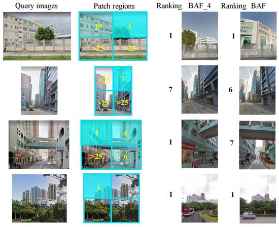
Figure 12.
Improvement of patch-region retrieval method to the results: in improvement of ranking of the correct results.
For DeLF, the experimental results of DeLF_4 are better than those of DeLF except Recall@2 and Recall@8. And results of DELF_4 have achieved the maximum increase of 2.67% in between Recall@19 and Recall@22.
On the whole, patch-region retrieval method significantly improved retrieval performance both of DeLF and BAF.
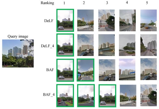
Figure 13.
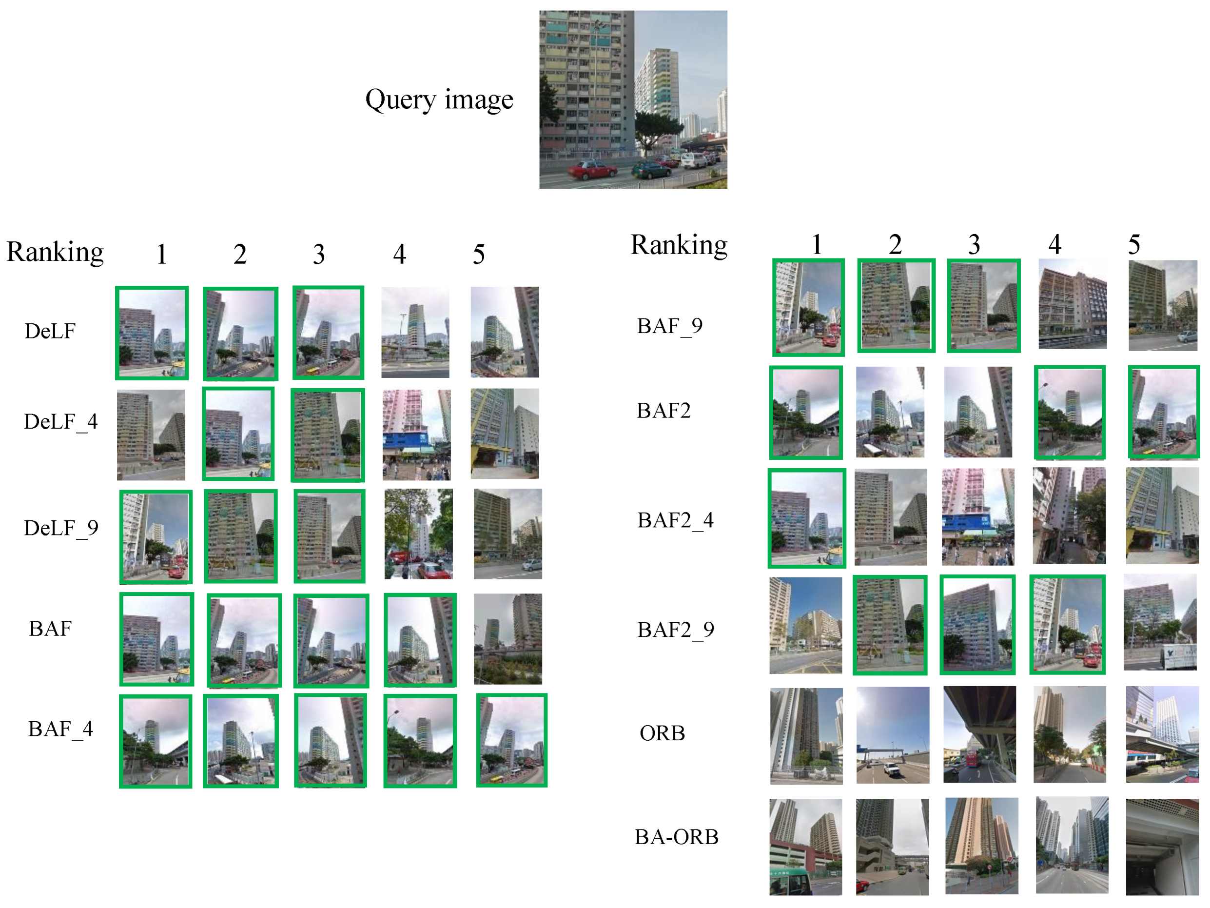
Top5 location result of same query image is used to show effectiveness of BAF descriptor.
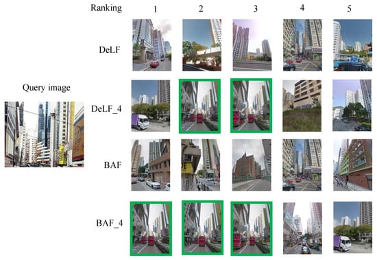
Figure 14.
Top5 location result of same query image is used to show effectiveness of patch-region retrieval.
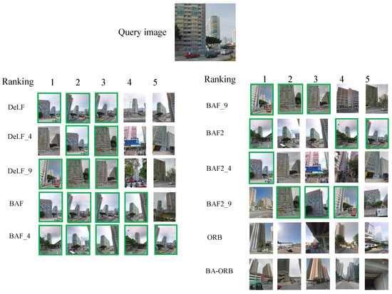
Figure 15.
A street-level image queried in 11 ways.
The positioning of the above query image is difficult in Figure 14, and the top 5 retrieval results of DeLF and BAF did not complete this localization task. However, the introduction of patch-region retrieval method not only completes the location of the query image, but also correctly locates the top several names. The first three localization results of BAF_4 are correct.
In the query results of DeLF and DeLF_4 in Figure 13, the similarity between the result images ranked 1–5 is not high. Most of the correct results appear at the top of the ranked images list. Judging by the surrounding scene in the query image in Figure 13, it was not taken in a multilane parallel section. This shows that in the database, there are fewer street-level sampling-points near the location where the correct query results are located. It proves the success of sparse work. The ranking of the correct results also proves the validity of BAF and patch-region retrieval.
Street-level image sampling points have dense distribution patterns in multilane parallel and core sections. This leads to a high similarity of street-level images on these sections. Our sparse strategy is to interval sample points in independently numbered roads. So, our sparse work is limited by multilane parallel sections with dense sample points. Therefore, in the experiment results of BAF_4 showing in Figure 14, we can see that the top three pictures have a greater similarity. The query image of Figure 15 was taken in a multilane parallel section, so there is a similar situation in the ranked 1–5 images of the query results.
4.4. Compare with Hand-Crafted Feature
ORB [32] is a hand-crafted feature. In the field of image recognition and image matching, deep learning features are better than manual features recent years. Our core inspiration comes from these papers [4,27,41], they are all deep learning methods. Their experiments have basically no manual features. Works of DeLF compare DIR, a hand-crafted feature. After adding QE [27], the precision of DIR is less than 20%. The dataset using in this experiment is also a large-scale dataset—Google landmark dataset. BAF is a deep learning feature and is 40-dimensional. Its network comes from the ResNet series, which is known for its depth. We believe that the deep network can learn more representative features. At the same time, it can still maintain robustness in metropolitan-scale and complex dataset. Our experiment also proved our point. Simply put, BAF is better than ORB.
5. Conclusions
When dealing with IBL task under urban scene, existing methods do not contain specific optimization for street-level images, whether in the stage of feature extraction or in the stage of geometric verification. The complex scenes in the street-level images are not conducive to the simplicity of the extracted features. If features extracted from street-level images are all used for matching, those are falling on meaningless objects will cause negative effects on localization accuracy. At the same time, the IBL method designed needs to have robustness and engineering value under the data scale of megacity. Our work is based on metropolitan-scale street-level images. We focus on the application of deep learning methods using in IBL tasks. Through experiments, it is also proved that hand-crafted features are not suitable for our application scenarios and method framework. Compared with that of real-time positioning and three-dimensional positioning, our method has differences in data composition, accuracy requirements, and application scope. Our work has application value in transportation planning, emergency response, image search, etc. Considering problems above, this paper made following contributions: (1) buildings play an important role in the discrimination of street scene scenes, and this paper proposes the Building-Aware Feature (BAF), which has building-sensitive characteristics. BAF cannot improve the recall of correct image positioning of street-level images, and it also shows competitiveness in the storage space and retrieval time. In our experiment, BAF guarantees the highest accuracy before Recall@12. (2) To further optimize the geometric verification stage and improve retrieval recall, we put forward Patch-Region Retrieval (PRR). PRR can optimize the efficiency of iterative operations in the geometric verification stage, as well as improve the retrieval performance of BAF and other features in our dataset. We fully demonstrated the validity of BAF and PRR through experiments with our dataset. As the dataset we collected holds metropolitan-scale and data-diversity, our method is demonstrably practical.
Author Contributions
Conceptualization, Y.Q., Z.X.; methodology, Y.Q.; software, L.Z. and L.Q.; validation, Y.Q.; formal analysis, Y.Q.; investigation, L.Z., Y.Q. and L.Q.; resources, Y.Q.; data curation, L.Z. and Y.Q.; writing—original draft preparation, Y.Q.; writing—review and editing, L.Z., Y.Q.; visualization, L.Z., Y.Q.; supervision, Z.X., Y.Q.; project administration, Z.X. and Y.Q.; funding acquisition, Z.X., Y.Q.; All authors have read and agreed to the published version of the manuscript.
Funding
This research received no external funding.
Institutional Review Board Statement
Not applicable.
Informed Consent Statement
Informed consent was obtained from all subjects involved in the study.
Data Availability Statement
Restrictions apply to the availability of these data. Data was obtained from Google Map at public networkand are available at https://www.google.com/maps/?hl=zh-cn.
Acknowledgments
The numerical calculations in this paper were performed on the supercomputing system in the Supercomputing Center of Wuhan University.
Conflicts of Interest
The authors declare no conflict of interest.
References
- Wu, Y.; Chen, Y.; Yuan, L.; Liu, Z.; Wang, L.; Li, H.; Fu, Y. Rethinking Classification and Localization in R-CNN. CoRR 2019. Available online: http://xxx.lanl.gov/abs/1904.06493 (accessed on 7 October 2021).
- Huang, X.; He, B.; Tong, M.; Wang, D.; He, C. Few-Shot Object Detection on Remote Sensing Images via Shared Attention Module and Balanced Fine-Tuning Strategy. Remote Sens. 2021, 13, 3816. [Google Scholar] [CrossRef]
- Yang, C.; Wu, Z.; Zhou, B.; Lin, S. Instance Localization for Self-supervised Detection Pretraining. CoRR 2021. Available online: https://arxiv.org/abs/2102.08318 (accessed on 7 October 2021).
- Ge, Y.; Wang, H.; Zhu, F.; Zhao, R.; Li, H. Self-supervising Fine-grained Region Similarities for Large-scale Image Localization. CoRR 2020. Available online: https://arxiv.org/abs/2006.03926 (accessed on 7 October 2021).
- Zhang, M.; Maidment, T.; Diab, A.; Kovashka, A.; Hwa, R. Domain-robust VQA with Diverse Datasets and Methods but No Target Labels. In Proceedings of the IEEE/CVF Conference on Computer Vision and Pattern Recognition (CVPR), Kuala Lumpur, Malaysia, 19 June 2021. [Google Scholar]
- Xu, L.; Huang, H.; Liu, J. TrafficQA: A Question Answering Benchmark and an Efficient Network for Video Reasoning over Traffic Events. CoRR 2021. Available online: https://arxiv.org/abs/2103.15538 (accessed on 7 October 2021).
- Singh Chaplot, D.; Salakhutdinov, R.; Gupta, A.; Gupta, S. Neural Topological SLAM for Visual Navigation. In Proceedings of the IEEE/CVF Conference on Computer Vision and Pattern Recognition (CVPR), Seattle, WA, USA, 13 June 2020; pp. 12872–12881. [Google Scholar] [CrossRef]
- Liu, L.; Li, H.; Dai, Y. Stochastic Attraction-Repulsion Embedding for Large Scale Image Localization. In Proceedings of the IEEE/CVF International Conference on Computer Vision (ICCV), Seoul, Korea, 27 October 2019; pp. 2570–2579. [Google Scholar] [CrossRef] [Green Version]
- Kim, H.J.; Dunn, E.; Frahm, J.M. Learned Contextual Feature Reweighting for Image Geo-Localization. In Proceedings of the IEEE Conference on Computer Vision and Pattern Recognition (CVPR), Honolulu, HI, USA, 21–26 July 2017; pp. 3251–3260. [Google Scholar] [CrossRef]
- Zheng, Z.; Wei, Y.; Yang, Y. University-1652: A Multi-view Multi-source Benchmark for Drone-based Geo-localization. CoRR 2020. Available online: http://xxx.lanl.gov/abs/2002.12186 (accessed on 7 October 2021).
- Wang, P.; Yang, R.; Cao, B.; Xu, W.; Lin, Y. DeLS-3D: Deep Localization and Segmentation with a 3D Semantic Map. CoRR 2018. Available online: http://arxiv.org/abs/1805.04949 (accessed on 7 October 2021).
- Schönberger, J.L.; Pollefeys, M.; Geiger, A.; Sattler, T. Semantic Visual Localization. CoRR 2017. Available online: http://arxiv.org/abs/1712.05773 (accessed on 7 October 2021).
- Cheng, X.; Liu, L.; Song, C. A Cyclic Information–Interaction Model for Remote Sensing Image Segmentation. Remote Sens. 2021, 13, 3871. [Google Scholar] [CrossRef]
- Liu, L.; Li, H.; Dai, Y. Efficient Global 2D-3D Matching for Camera Localization in a Large-Scale 3D Map. In Proceedings of the IEEE International Conference on Computer Vision (ICCV), Venice, Italy, 22 October 2017; pp. 2391–2400. [Google Scholar] [CrossRef]
- Sattler, T.; Leibe, B.; Kobbelt, L. Improving Image-Based Localization by Active Correspondence Search. In Computer Vision—ECCV 2012; Fitzgibbon, A., Lazebnik, S., Perona, P., Sato, Y., Schmid, C., Eds.; Springer: Berlin/Heidelberg, Germany, 2012; pp. 752–765. [Google Scholar]
- Seo, P.H.; Weyand, T.; Sim, J.; Han, B. CPlaNet: Enhancing Image Geolocalization by Combinatorial Partitioning of Maps. CoRR 2018. Available online: http://xxx.lanl.gov/abs/1808.02130 (accessed on 7 October 2021).
- Lowe, D. Distinctive Image Features from Scale-Invariant Keypoints. Int. J. Comput. Vis. 2004, 60, 91. [Google Scholar] [CrossRef]
- Bay, H.; Ess, A.; Tuytelaars, T.; Van Gool, L. Speeded-Up Robust Features (SURF). Comput. Vis. Image Underst. 2008, 110, 346–359. [Google Scholar] [CrossRef]
- Jégou, H.; Perronnin, F.; Douze, M.; Sánchez, J.; Pérez, P.; Schmid, C. Aggregating Local Image Descriptors into Compact Codes. IEEE Trans. Pattern Anal. Mach. Intell. 2012, 34, 1704–1716. [Google Scholar] [CrossRef] [Green Version]
- Arandjelović, R.; Gronat, P.; Torii, A.; Pajdla, T.; Sivic, J. NetVLAD: CNN Architecture for Weakly Supervised Place Recognition. IEEE Trans. Pattern Anal. Mach. Intell. 2018, 40, 1437–1451. [Google Scholar] [CrossRef] [Green Version]
- Xu, Y.; Chen, R.; Gotsman, C.; Liu, L. Embedding a triangular graph within a given boundary. Comput. Aided Geom. Des. 2011, 28, 349–356. [Google Scholar] [CrossRef]
- Babenko, A.; Lempitsky, V.S. Aggregating Deep Convolutional Features for Image Retrieval. CoRR 2015. Available online: http://xxx.lanl.gov/abs/1510.07493 (accessed on 7 October 2021).
- Tolias, G.; Sicre, R.; Jégou, H. Particular object retrieval with integral max-pooling of CNN activations. arXiv 2015, arXiv:1511.05879. [Google Scholar]
- Zhu, H.; Jiao, L.; Ma, W.; Liu, F.; Zhao, W. A Novel Neural Network for Remote Sensing Image Matching. IEEE Trans. Neural Networks Learn. Syst. 2019, 30, 2853–2865. [Google Scholar] [CrossRef]
- Ng, T.; Balntas, V.; Tian, Y.; Mikolajczyk, K. SOLAR: Second-Order Loss and Attention for Image Retrieval. CoRR 2020. Available online: https://arxiv.org/abs/2001.08972 (accessed on 7 October 2021).
- Fischler, M.A.; Bolles, R.C. Random Sample Consensus: A Paradigm for Model Fitting with Applications to Image Analysis and Automated Cartography. In Readings in Computer Vision; Fischler, M.A., Firschein, O., Eds.; Morgan Kaufmann: San Francisco, CA, USA, 1987; pp. 726–740. [Google Scholar] [CrossRef]
- Noh, H.; Araujo, A.; Sim, J.; Weyand, T.; Han, B. Large-Scale Image Retrieval with Attentive Deep Local Features. In Proceedings of the IEEE International Conference on Computer Vision (ICCV), Venice, Italy, 22 October 2017; pp. 3476–3485. [Google Scholar] [CrossRef] [Green Version]
- Zheng, L.; Yang, Y.; Tian, Q. SIFT Meets CNN: A Decade Survey of Instance Retrieval. IEEE Trans. Pattern Anal. Mach. Intell. 2018, 40, 1224–1244. [Google Scholar] [CrossRef] [Green Version]
- Tolias, G.; Jenícek, T.; Chum, O. Learning and aggregating deep local descriptors for instance-level recognition. CoRR 2020. Available online: https://arxiv.org/abs/2007.13172 (accessed on 7 October 2021).
- Zheng, Y.T.; Zhao, M.; Song, Y.; Adam, H.; Buddemeier, U.; Bissacco, A.; Brucher, F.; Chua, T.S.; Neven, H. Tour the world: Building a web-scale landmark recognition engine. In Proceedings of the IEEE Conference on Computer Vision and Pattern Recognition, Miami, FL, USA, 20–25 June 2009; pp. 1085–1092. [Google Scholar] [CrossRef]
- Teichmann, M.; Araujo, A.; Zhu, M.; Sim, J. Detect-to-Retrieve: Efficient Regional Aggregation for Image Search. CoRR 2018. Available online: http://xxx.lanl.gov/abs/1812.01584 (accessed on 7 October 2021).
- Rublee, E.; Rabaud, V.; Konolige, K.; Bradski, G. ORB: An efficient alternative to SIFT or SURF. In Proceedings of the International Conference on Computer Vision, Barcelona, Spain, 6–13 November 2011; pp. 2564–2571. [Google Scholar] [CrossRef]
- Ren, S.; He, K.; Girshick, R.; Sun, J. Faster R-CNN: Towards Real-Time Object Detection with Region Proposal Networks. IEEE Trans. Pattern Anal. Mach. Intell. 2017, 39, 1137–1149. [Google Scholar] [CrossRef] [Green Version]
- Siméoni, O.; Avrithis, Y.; Chum, O. Local Features and Visual Words Emerge in Activations. CoRR 2019. Available online: http://arxiv.org/abs/1905.06358 (accessed on 7 October 2021).
- Cao, B.; Araujo, A.; Sim, J. Unifying Deep Local and Global Features for Efficient Image Search. CoRR 2020. Available online: https://arxiv.org/abs/2001.05027 (accessed on 7 October 2021).
- Vapnik, V.; Chervonenkis, A. A note on one class of perceptrons. Autom. Remote Control 1964, 25. Available online: http://www.kernel-machines.org/publications/VapChe64 (accessed on 7 October 2021).
- Boser, B.E.; Guyon, I.M.; Vapnik, V.N. A Training Algorithm for Optimal Margin Classifiers. In Proceedings of the 5th Annual ACM Workshop on COLT, Pittsburgh, PA, USA, 27–29 July 1992; Haussler, D., Ed.; ACM Press: Pittsburgh, PA, USA, 1992; pp. 144–152. [Google Scholar]
- Faugeras, O.D. What can be seen in three dimensions with an uncalibrated stereo rig? In Computer Vision—ECCV’92; Sandini, G., Ed.; Springer: Berlin/Heidelberg, Germany, 1992; pp. 563–578. [Google Scholar]
- Philbin, J.; Chum, O.; Isard, M.; Sivic, J.; Zisserman, A. Object retrieval with large vocabularies and fast spatial matching. In Proceedings of the IEEE Conference on Computer Vision and Pattern Recognition, Minneapolis, MN, USA, 17–22 June 2007; pp. 1–8. [Google Scholar] [CrossRef]
- Philbin, J.; Chum, O.; Isard, M.; Sivic, J.; Zisserman, A. Lost in quantization: Improving particular object retrieval in large scale image databases. In Proceedings of the IEEE Conference on Computer Vision and Pattern Recognition, Anchorage, AK, USA, 23–28 June 2008; pp. 1–8. [Google Scholar] [CrossRef] [Green Version]
- Torii, A.; Arandjelović, R.; Sivic, J.; Okutomi, M.; Pajdla, T. 24/7 Place Recognition by View Synthesis. IEEE Trans. Pattern Anal. Mach. Intell. 2018, 40, 257–271. [Google Scholar] [CrossRef] [Green Version]
- Zhao, H.; Shi, J.; Qi, X.; Wang, X.; Jia, J. Pyramid Scene Parsing Network. In Proceedings of the IEEE Conference on Computer Vision and Pattern Recognition (CVPR), Honolulu, HI, USA, 21–26 July 2017; pp. 6230–6239. [Google Scholar] [CrossRef] [Green Version]
- He, K.; Zhang, X.; Ren, S.; Sun, J. Deep Residual Learning for Image Recognition. In Proceedings of the IEEE Conference on Computer Vision and Pattern Recognition (CVPR), Las Vegas, NV, USA, 27–30 June 2016; pp. 770–778. [Google Scholar] [CrossRef] [Green Version]
- Dugas, C.; Bengio, Y.; Bélisle, F.; Nadeau, C.; Garcia, R. Incorporating Second-Order Functional Knowledge for Better Option Pricing. In Proceedings of the Advances in Neural Information Processing Systems 13, Papers from Neural Information Processing Systems (NIPS), Denver, CO, USA, 1 January 2000; pp. 472–478. [Google Scholar]
- Neubeck, A.; Gool, L. Efficient Non-Maximum Suppression. In Proceedings of the 18th International Conference on Pattern Recognition (ICPR’06), Hong Kong, China, 20–24 August 2006; Volume 3, pp. 850–855. [Google Scholar]
- Jégou, H.; Chum, O. Negative Evidences and Co-occurences in Image Retrieval: The Benefit of PCA and Whitening. In Computer Vision–ECCV 2012; Fitzgibbon, A., Lazebnik, S., Perona, P., Sato, Y., Schmid, C., Eds.; Springer: Berlin/Heidelberg, Germany, 2012; pp. 774–787. [Google Scholar]
- Qin, J.; He, Z.S. A SVM face recognition method based on Gabor-featured key points. In Proceedings of the International Conference on Machine Learning and Cybernetics, Guangzhou, China, 18–21 August 2005; Volume 8, pp. 5144–5149. [Google Scholar] [CrossRef]
- Jégou, H.; Douze, M.; Schmid, C. Product Quantization for Nearest Neighbor Search. IEEE Trans. Pattern Anal. Mach. Intell. 2011, 33, 117–128. [Google Scholar] [CrossRef] [Green Version]
- Sivic, J.; Zisserman, A. Video Google: A text retrieval approach to object matching in videos. In Proceedings of the Ninth IEEE International Conference on Computer Vision, Nice, France, 13–16 October 2003; Volume 2, pp. 1470–1477. [Google Scholar] [CrossRef]
- Lin, P.; Zhao, W. A Comparative Study on Hierarchical Navigable Small World Graphs. arXiv 2019, arXiv:1904.02077. [Google Scholar]
- Ram, P.; Sinha, K. Revisiting kd-tree for Nearest Neighbor Search. In Proceedings of the 25th ACM Sigkdd International Conference on Knowledge Discovery & Data Mining, Anchorage, AK, USA, 25 July 2019. [Google Scholar] [CrossRef]
- Hadjieleftheriou, M.; Manolopoulos, Y.; Theodoridis, Y.; Tsotras, V.J. R-Trees—A Dynamic Index Structure for Spatial Searching. In Encyclopedia of GIS; Shekhar, S., Xiong, H., Eds.; Springer: Boston, MA, USA, 2008; pp. 993–1002. [Google Scholar] [CrossRef]
- Wang, F.E.; Hu, H.N.; Cheng, H.T.; Lin, J.T.; Yang, S.T.; Shih, M.L.; Chu, H.K.; Sun, M. Self-supervised Learning of Depth and Camera Motion from 360°Videos. In Computer Vision–ACCV 2018; Jawahar, C., Li, H., Mori, G., Schindler, K., Eds.; Springer International Publishing: Cham, Switzerland, 2019; pp. 53–68. [Google Scholar]
- Cordts, M.; Omran, M.; Ramos, S.; Rehfeld, T.; Enzweiler, M.; Benenson, R.; Franke, U.; Roth, S.; Schiele, B. The Cityscapes Dataset for Semantic Urban Scene Understanding. In Proceedings of the IEEE Conference on Computer Vision and Pattern Recognition (CVPR), Las Vegas, NV, USA, 27–30 June 2016; pp. 3213–3223. [Google Scholar] [CrossRef] [Green Version]
Publisher’s Note: MDPI stays neutral with regard to jurisdictional claims in published maps and institutional affiliations. |
© 2021 by the authors. Licensee MDPI, Basel, Switzerland. This article is an open access article distributed under the terms and conditions of the Creative Commons Attribution (CC BY) license (https://creativecommons.org/licenses/by/4.0/).


