PM_2.5 Concentration Forecasting over the Central Area of the Yangtze River Delta Based on Deep Learning Considering the Spatial Diffusion Process

Abstract

Precise PM_2.5 concentration forecasting is significant to environmental management and human health. Researchers currently add various parameters to deep learning models for PM_2.5 concentration forecasting, but most of them ignore the problem of PM_2.5 concentration diffusion. To address this issue, a deep learning model-based PM_2.5 concentration forecasting method considering the diffusion process is proposed in this paper. We designed a spatial diffuser to express the diffusion process of gaseous pollutants; that is, the concentration of PM_2.5 in four surrounding directions was taken as the explanatory variable. The information from the target and associated stations was then employed as inputs and fed into the model, together with meteorological features and other pollutant parameters. The hourly data from 1 January 2019 to 31 December 2019, and the central area of the Yangtze River Delta, were used to conduct the experiment. The results showed that the forecasting performance of the method we proposed is superior to that of ignoring diffusion, with an average RMSE = 8.247 μg/m³ and average R² = 0.922 in three different deep learning models, RNN, LSTM, and GRU, in which RMSE decreased by 10.52% and R² increased by 2.22%. Our PM_2.5 concentration forecasting method, which was based on an understanding of basic physical laws and conformed to the characteristics of data-driven models, achieved excellent performance.

1. Introduction

While rapid industrialization and urbanization have made a positive impact worldwide, there have also been various negative effects, such as environmental degradation [1,2,3], where air pollution has aroused people’s great concern in China. Air quality refers to the degree of atmospheric pollution, which is commonly expressed by the air quality index (AQI) [4]. The AQI is a dimensionless and artificially defined index whose value is calculated by the concentration of pollutants in the atmosphere. At present, there are six pollutants used to calculate the AQI in China, PM_2.5, PM₁₀, SO₂, NO₂, CO, and O₃. Among these pollutants, fine particulate matter 2.5 (PM_2.5, aerodynamic diameter ≤ 2.5 μm) has gradually become the primary pollutant in most cities. Studies [5,6] show that PM_2.5 can pass through human nasal passages to reach the throat and even the deep part of the lungs, which will cause severe lung and cardiovascular diseases. PM_2.5 is extremely harmful to people’s health. Therefore, it is extremely important to accurately forecast the value of PM_2.5 concentration in the approaching time to reduce people’s exposure to it.

A wide variety of methods have been used to forecast or predict the concentration of PM_2.5, and they can be classified into two major classes [7]: physical-based methods and data-driven methods. The physics-based model is the chemical transport model (CTM) [8], which is based on the principles of meteorological and mathematical statistical methods. The model also uses atmospheric physical and chemical reactions in the process of pollutant discharge, diffusion, transformation, and dissipation to simulate the diffusion and migration mechanism of air pollutants to predict air pollution [9,10]. While they can provide valuable insights into the mechanisms of pollutant diffusion, their use is limited because the dynamic mechanism on which most deterministic models are based is very complex and requires the setting of numerous parameters [11].

Compared with physical-based models, data-driven models have their own characteristics. While physical-based models have a better understanding of mechanism processes, data-driven models are statistical models based on historical data that can obtain better forecast results as long as there are enough data [6]. We believe that statistical models overcome some limitations of the physical-based model. The traditional statistical models [12,13,14,15] that can be used to forecast PM_2.5 concentrations are multiple linear regression (MLR), generalized additive models (GAMs), geographically weighted regression (GWR), and their combinations and deformation. In recent years, with the development of computer science, machine learning models, especially deep learning models, have become prominent in PM_2.5 concentration forecasting due to their advantageous ability to simulate nonlinear processes. Examples of models usually used include the Markov model (HMM) [16], spatiotemporal support vector machine model (SVM) [17], recurrent neural network (RNN) [18], random forests (RF) [19], and artificial neural network method (ANN) [20], as well as their combinations and deformation. Among these models, RF has the best performance in machine learning models and RNN is particularly suitable for capturing the laws of the spatiotemporal evolution of PM_2.5, due to the characteristics of time series data. Ibai Laña et al. [19] used RF method to study the relationship between traffic and meteorological conditions and air pollution. Joanna A et al. [21] used a partition RF method to predict the concentration of NO₂, and its accuracy was better than that of classical random forest method. Shang et al. [22] developed a new structure based on RF and obtained good results. Meanwhile, [23,24,25] proposed RNN can process input sequences of any length and ensure the ability to learn time sequences. However, the traditional RNN cannot capture the long-term dependence, which makes it difficult to train the RNN for a long time due to the disappearance of the slope and the explosion of the gradient, meaning that the RNN has only short-term memory.

To improve these problems, Hochreiter and Schmidhuber [26] developed the long short-term memory (LSTM) neural network, a new RNN architecture. Different from traditional RNN, LSTM has the ability to learn a long time series because it is not easily affected by the vanishing gradient problem, which is particularly important for modeling the change in PM_2.5. Later, many scholars improved the LSTM model from different angles. Li et al. [27] applied this model to forecast air pollution concentrations and showed an excellent performance. Zhang et al. [28] constructed an E-BI-LSTM model to forecast PM_2.5 concentrations. At the same time, they revealed the correlation between multiple climate features and PM_2.5 concentration. Chang et al. [29] summarized SVM, GBTR, and LSTM into ALSTM to improve the accuracy of forecasting. The Abirami S et al. [30] layer deep learning model using DL-AIR included STAA-LSTM, a variant of LSTM, which improved forecast accuracy. The model structure of the gated recurrent unit (GRU) [31] proposed in 2014 by Cho is the deformation of the LSTM model, but the GRU design is simpler. Tao et al. [32] applied the combination of convolutional neural network and GRU to predict PM_2.5 concentration. Huang et al. [33] constructed a multi-step prediction GRU neural network combining with using empirical mode decomposition (EMD) to decompose the PM_2.5 concentration series and achieved better results.

As mentioned above, for the forecast of PM_2.5 concentration, many scholars have improved the forecast model from various mathematical transformations of PM_2.5 concentration series data, various transformations of the deep learning, and the addition of various meteorological and geographical parameters. They have also made considerable achievements and massively improved the forecast accuracy, but in regard to what kind of parameters should be taken as inputs of the model, rarely have they taken the nearby stations’ PM_2.5 concentration data into account. As a well-known observation [34], when there is pollution from one source of gas, the pollution will spread out, and the diffusion process is captured by adjacent stations.

Therefore, we first propose a spatial diffuser to organize data from nearby stations to construct PM_2.5 multifeature temporal datasets. Moreover, the correlation between the central stations and neighboring stations is evaluated as the basis for model construction. In addition, the RNN, LTSM, and GRU approaches are used to evaluate the forecast accuracy of the spatial diffuser, as well as its generalizability. The goal of this paper is to use the spatial diffuser to extract PM_2.5 concentration data of adjacent stations that represent the diffusion process and use it to construct feature datasets as the input of the model. This work provides a new solution of thinking about adjacent stations data as inputs to model parameters.

2. Study Area and Materials

2.1. Study Area

The Yangtze River Delta is one of the areas with the most active economy and the fastest urbanization in China. On 1 December 2019, China issued the Outline for the Integrated Development of the Yangtze River Delta Region. The central area of the Yangtze River Delta encompasses 27 cities in Jiangsu, Anhui, Zhejiang, and Shanghai, with an area of 225 thousand square kilometers. The spatial extent is 27°10′–34°30′N; 115°44′–122°31′E (Figure 1). Various factories are distributed here, which also brings many pollution problems. According to data from the Ministry of Environmental Protection of China [35], the Yangtze River Delta is an area with relatively heavy air pollution. PM_2.5 pollution reduces atmospheric visibility, affects human health to a large extent, and even impacts global climate change. Therefore, the central area of the Yangtze River Delta was selected as the study area of this paper.

2.2. Data Source

2.2.1. Air Quality Data

We downloaded the hourly PM_2.5 concentration data of 167 stations in the study area from 1 January to 31 December 2019, which can be obtained through the National Urban Air Quality Real-time Release Platform at: http://106.37.208.233:20035/ (accessed on 24 February 2021). At the same time, we downloaded the data of other gas pollutants, including SO₂, NO₂, CO, and O₃ data.

Table 1. Descriptive statistics of pollutant concentration parameters.

Parameters	Unit	Range	Average	St. Dev.
PM2.5	μg/m3	(1, 690]	35.88	30.25
PM10	μg/m3	[1, 1017]	55.52	46.02
SO2	μg/m3	[1, 777]	7.75	7.41
NO2	μg/m3	[1, 545]	32.89	24.93
CO	mg/m3	[1, 700]	59.64	48.95
O3	μg/m3	[1, 300]	58.37	43.82

shows the descriptive statistics of PM_2.5 concentrations, along with the other measured variables. The unit of CO is mg/m³ and the unit of other gas pollutants is ug/m³.

2.2.2. Meteorological Data

Meteorological factors play a pivotal role in the formation, dispersion, and transport of PM_2.5 at regional and local scales [36]. We extracted meteorological parameters from the ERA5 reanalysis. ERA5 data are provided on regular latitude–longitude grids at approximately 28 km × 28 km resolution (0.25° × 0.25°) and up to 1 h frequency, which is the same as the air quality data. The data can be retrieved from the ECMWF at: https://cds.climate.copernicus.eu/ (accessed on 10 May 2021). We collected these parameters from 1 January to 31 December 2019, in the central area of the Yangtze River Delta, including a daily minimum of 2 m dewpoint temperature (d2m), 2 m temperature (t2m), wind speed and direction (10 m u-component of wind and 10 m v-component of wind, u10 and v10), boundary layer height (blh), total cloud cover (tcc), and total precipitation (tp).

3. Methodology

3.1. Establishing the Dataset

3.1.1. Influence on the PM_2.5 Concentration Feature Selection

Weather conditions and the concentration of other pollutants are important factors that affect the migration and transformation of PM_2.5 [37]; meanwhile, many parameters affect PM_2.5 concentration, and the process is very complicated. Therefore, to narrow the selection range of influencing factors and determine the main influencing factors, before forecasting the PM_2.5 concentration, it is extremely important to analyze the relevant parameters to achieve better forecasting results. The Pearson correlation coefficient [38] was selected as the measurement index to evaluate the meteorological parameters and other pollutant parameters related to the PM_2.5 concentration. Equation (1) is the calculation method of the Pearson correlation coefficient, where x represents the concentration values of PM_2.5 and y represents the values of other data. n is the amount of each data.

$${\mathsf{\rho }}_{\mathrm{x},\mathrm{y}}=\frac{\mathrm{n}{{\displaystyle \sum }}_{\mathrm{i}=1}^{\mathrm{n}}{\mathrm{x}}_{\mathrm{i}}{\mathrm{y}}_{\mathrm{i}}-{{\displaystyle \sum }}_{\mathrm{i}=1}^{\mathrm{n}}{\mathrm{x}}_{\mathrm{i}}{{\displaystyle \sum }}_{\mathrm{i}=1}^{\mathrm{n}}{\mathrm{y}}_{\mathrm{i}}}{\sqrt{\mathrm{n}{{\displaystyle \sum }}_{\mathrm{i}=1}^{\mathrm{n}}{\mathrm{x}}_{\mathrm{i}}^2-{\left({{\displaystyle \sum }}_{\mathrm{i}=1}^{\mathrm{n}}{\mathrm{x}}_{\mathrm{i}}\right)}^2}\sqrt{\mathrm{n}{{\displaystyle \sum }}_{\mathrm{i}=1}^{\mathrm{n}}{\mathrm{y}}_{\mathrm{i}}^2-{\left({{\displaystyle \sum }}_{\mathrm{i}=1}^{\mathrm{n}}{\mathrm{y}}_{\mathrm{i}}\right)}^2}}$$

(1)

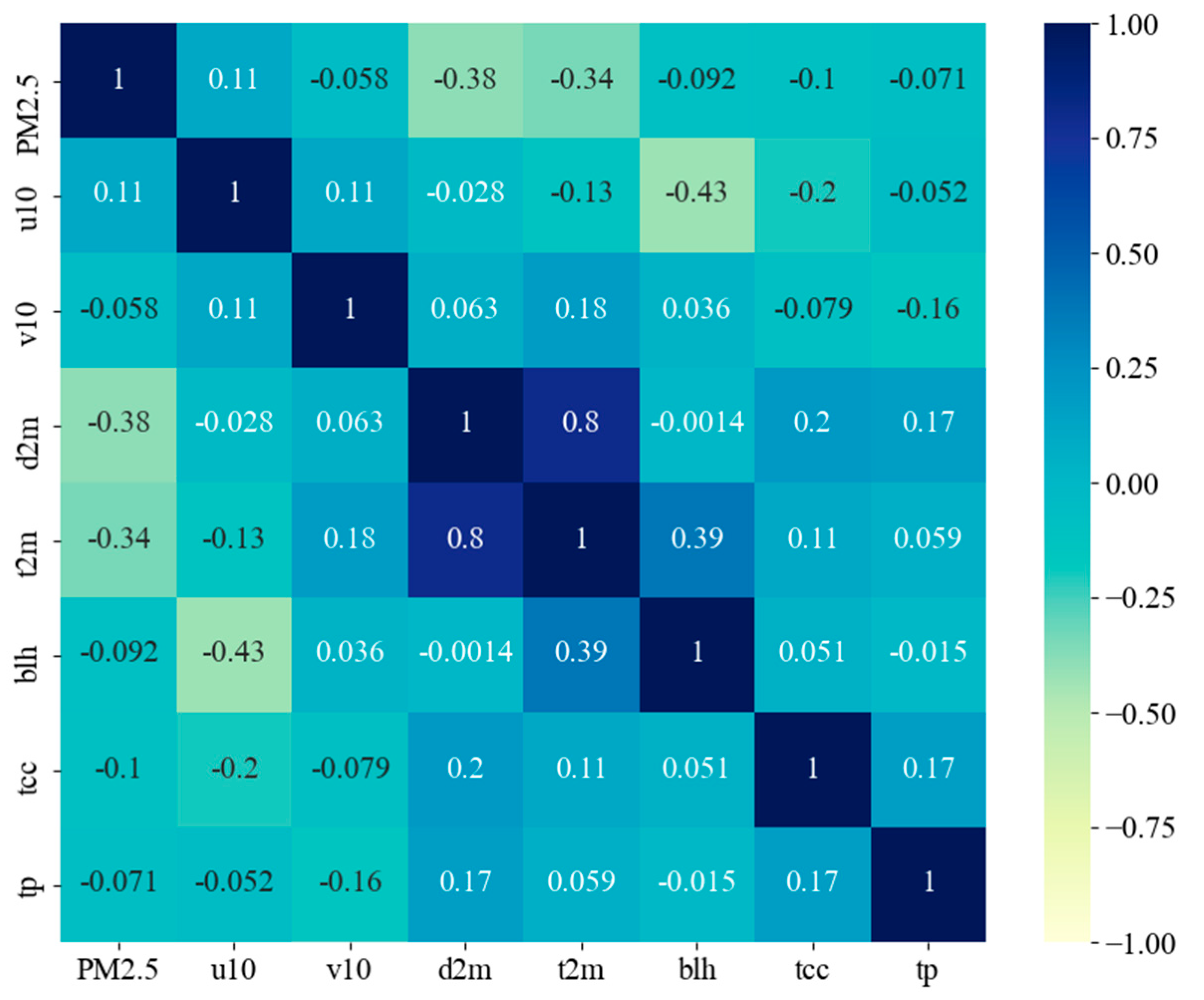
Figure 2 reflects the relationship between PM_2.5 concentrations and meteorological environment fields, whose correlation coefficient is expressed in the form of a heatmap. As shown in Figure 2, d2m and t2m have the highest correlation coefficients with PM_2.5 concentrations among those meteorological environment fields, indicating that temperature and humidity may have a strong relationship with the content of PM_2.5 in the atmosphere. Moreover, wind has a certain influence on the concentration of PM_2.5, and the influence of meridional wind is greater than that of zonal wind. In addition, in this study area, we found a higher correlation between tcc and PM_2.5 concentration than blh, which is different from the PM_2.5 concentration forecasting made by most researchers in other areas. In this paper, the correlation coefficients between the PM_2.5 concentration value and the selected meteorological environmental parameters all have a certain correlation. Then, u10, v10, d2m, t2m, tcc, tp, and blh are selected as the input data, together with the PM_2.5 concentration value data.

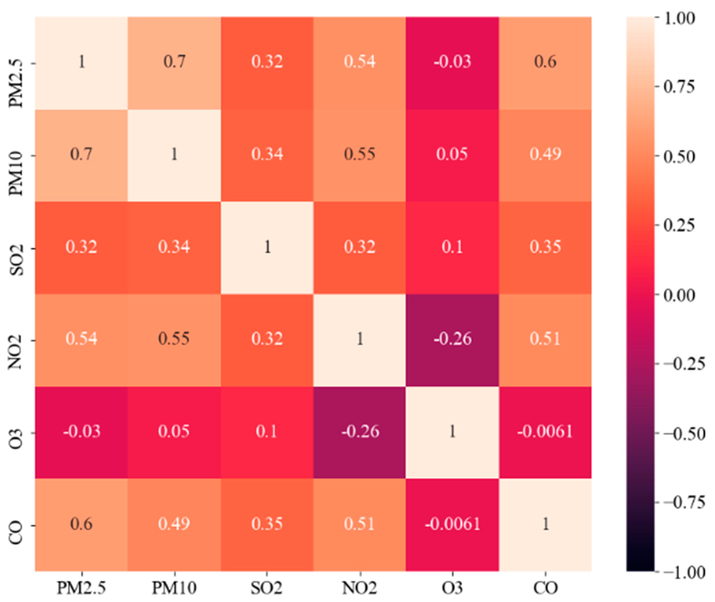
Similar to Figure 2, Figure 3 shows the correlation between PM_2.5 concentrations and other pollutant concentrations. As Figure 3 vividly shows, the correlation between the PM₁₀ concentration and the PM_2.5 concentration is considerably greater than that between the PM_2.5 concentration and SO₂, NO₂, and CO. This is also consistent with the studies [37] that showed that PM_2.5 is strongly positively correlated with PM₁₀. (R² = 0.87, P < 0.01). PM_2.5 accounts for approximately 65% of PM₁₀. In addition, there is a definitely correlation between the SO₂, NO_2, CO, and PM_2.5 concentration values, which means that they have an important influence on the translation of the PM_2.5 concentration value. For O₃, although the correlation coefficient is meager, compared with SO₂, NO₂, and CO, according to Lin Huang’s research [39], there is a complex relationship between PM_2.5 and O₃ that changes according to time scale. Therefore, PM₁₀, NO₂, CO, SO₂, and O₃ were chosen as the inputs and fed into the model.

3.1.2. Spatial Diffusion Process Expression

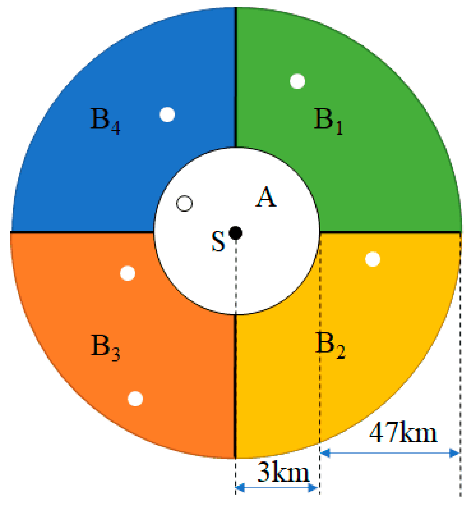
The generation, development, migration, and dissipation of PM_2.5 are affected by various factors. PM_2.5 concentrations at a single station are affected not only by meteorological environment fields but also by concentration differences in different regions. According to the latest environmental air quality standards [40] published by the Ministry of Environmental Protection, PRC, in 2012, the range of a single air quality monitoring station is approximately 3 km, while the average movement of the atmosphere in an hour is 50 km. Therefore, we designed a spatial diffuser model to express the spatial diffusion process of the PM_2.5 concentrations from high to low. The goal of the space diffuser was to forecast PM_2.5 concentrations at the central station in the next hour through the data from the neighboring stations.

During the construction of the space diffuser, as shown in Figure 4, we divided the circle into four areas using two perpendicular lines: northeast, southeast, southwest, and northwest. If the distance between the adjacent stations and the central station was less than 3 km, the adjacent stations was not be considered; if their distance was greater than 3 km and less than 50 km, they would be considered alternative stations; if there was only one station in a single region, the data of the station was taken as the value of the region; if there were multiple candidate sites in a single area, their average would be taken as the value of the area; if no site existed in a region, the central site would not meet the data requirements.

As shown in Figure 5, there is a strong correlation between the central station and surrounding stations, based on the spatial diffusion methods. We combined it with meteorological data and other pollutant parameter data to form a structured dataset.

3.1.3. Establishing the Dataset

Through the above exploration of the change in PM_2.5 concentration value at a station, we found that the PM_2.5 concentration value at a station was affected by the PM_2.5 concentration value at the station’s precursors, meteorological conditions, the concentration of other pollutants and the diffusion process, which can be further summarized as the mapping relationship of Equation (2):

$$\mathrm{y}\left(\mathrm{t}+\mathrm{n}\right)=\mathrm{f}(\mathrm{y}\left(\mathrm{t}\right),\cdots ,\mathrm{y}\left(\mathrm{t}-\mathrm{k}\right);\mathrm{z}\left(\mathrm{t}\right),\cdots \mathrm{z}\left(\mathrm{t}-\mathrm{k}\right);\mathrm{x}\left(\mathrm{t}\right),\cdots ,\mathrm{x}\left(\mathrm{t}-\mathrm{k}\right){;\mathrm{y}}_{\mathrm{near}}\left(\mathrm{t}\right),\cdots {\mathrm{y}}_{\mathrm{near}}(\mathrm{t}-\mathrm{k}))$$

(2)

where y represents the concentration of PM_2.5; z stands for the meteorological environment parameter value; x represents the concentration values of other pollutant parameters; y_near refers to the concentration of PM_2.5 at nearby stations; n is the forecasted time step; and k refers to the current time value.

The experiment used PM_2.5 concentration data from 1 January 2019, to 31 December 2019, as well as meteorological data provided by ERA5 reanalysis. The dataset belongs to a time series, covering thirteen features, including the u10, v10, d2m, t2m, tcc, tp, blh, PM_2.5, PM₁₀, SO₂, NO₂, CO₂, and O₃ concentrations. All data were spaced at 1 h intervals, and a total of 8760 h of data were produced. After eliminating 126,023 records containing missing values and 2 records with PM_2.5 concentrations greater than 600, we collected a total of 1,242,556 records. Then, for a control experiment, we made two sets of data, one that used a space diffuser and another that did not. There were 26 stations meeting the spatial diffuser. Thus, a total of 130,754 pairs of data were produced as the experimental dataset, while 130,754 pairs of the original data, without considering the diffusion process, were randomly selected as the experimental dataset. In this way, the two datasets were precisely the same size.

In the experiment, we divided the dataset into three parts: the first part was the training set, the second part was the validation set, and the third part was the test set. Their proportions to the original data were 40%, 30%, and 30%, respectively. When the amount of data in the training set reaches 15% of the total amount, loss function will not continue to decrease due to the increase in data in the training set. The training set was used to train the deep learning model parameters, and the model parameters were continuously optimized through the reduction in the loss function to improve the model performance. The validation set was used to avoid overfitting to evaluate the generalizability of the deep learning model. The effectiveness of the model was measured by the text set. All attributed data in the training set, validation set, and test set were standardized separately.

3.2. Forecasts Method

3.2.1. RNN Models

Recurrent neural network (RNN) architectures [26] are a kind of neural network for processing sequence data and have been widely used in various fields of processing and analyzing sequence data. Compared with the basic neural network structure, the RNN network structure is different in that weight connections are established between neurons and layers [20,21,22]. The basic RNN structure is shown in Figure 6, folded on the left and expanded on the right.

The RNN structure can be expressed by Equations (3) and (4) for time t:

$${\mathrm{h}}_{\mathrm{t}}=\tan \mathrm{h}\left({\mathrm{W}}_{\mathrm{h}}{\mathrm{h}}_{\mathrm{t}-1}{+\mathrm{W}}_{\mathrm{x}}{\mathrm{x}}_{\mathrm{t}}+\mathrm{b}\right)$$

(3)

$${\mathrm{y}}_{\mathrm{t}}{=\mathrm{W}}_{\mathrm{t}}{\mathrm{h}}_{\mathrm{t}}$$

(4)

where h_t is the hidden unit at time t, tanh is an activation function, and b is a bias vector. The weight matrices W_h are parameters for hidden state h, W_x are parameters for input x, and y_t is the experimental output vector.

3.2.2. LSTM Models

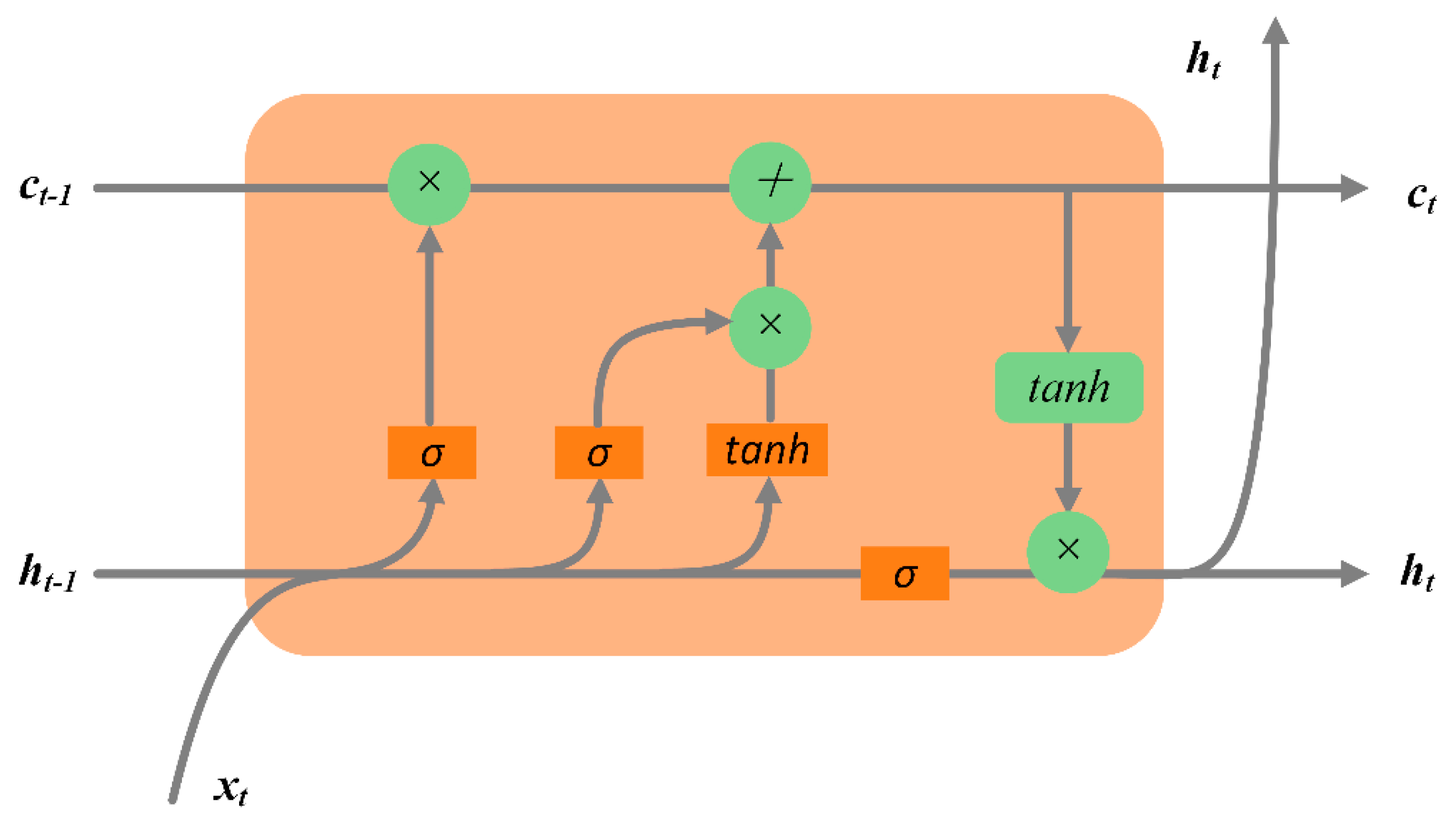
The long short-term memory (LSTM) [6] neural network is a special kind of RNN structure, which can solve the problem of long order dependence. The problem of long-term dependence and gradient disappearance is avoided by the deliberate design of cyclic layers. LSTM enhances the ability of simple recurrent neural networks to deal with distance-dependent problems by adding memory and control gates. The structure diagram of LSTM is shown in Figure 7. Like most RNNs, an LSTM network is universal in the sense that given enough network units it can compute anything a conventional computer can compute, provided it has the proper weight matrix, which may be viewed as its program. Unlike traditional RNN, an LSTM network is well-suited to learn from experience to classify, process, and predict time series when there are very longtime lags of unknown size between important events. This is one of the main reasons why LSTM outperforms alternative RNN and hidden Markov models and other sequence learning methods in numerous applications [41].

In Figure 7, the hidden state (h_t) of the LSTM cell is calculated as follows:

$${\mathrm{i}}_{\mathrm{t}}=\mathsf{\sigma }\left({\mathrm{W}}_{\mathrm{f}}\left[{\mathrm{h}}_{\mathrm{t}-1}{,\mathrm{x}}_{\mathrm{t}}\right]{+\mathrm{b}}_{\mathrm{i}}\right)$$

(5)

$${\mathrm{f}}_{\mathrm{t}}=\mathsf{\sigma }\left({\mathrm{W}}_{\mathrm{f}}\left[{\mathrm{h}}_{\mathrm{t}-1}{,\mathrm{x}}_{\mathrm{t}}\right]{+\mathrm{b}}_{\mathrm{f}}\right)$$

(6)

$$\mathrm{Sigmoid}=\frac{1}{{1+\mathrm{e}}^{-1}}$$

(7)

$${\mathrm{o}}_{\mathrm{t}}=\mathsf{\sigma }\left({\mathrm{W}}_{\mathrm{o}}\left[{\mathrm{h}}_{\mathrm{t}-1}{,\mathrm{x}}_{\mathrm{t}}\right]{+\mathrm{b}}_{\mathrm{o}}\right)$$

(8)

$$\widetilde{{\mathrm{c}}_{\mathrm{t}} }=\tan \mathrm{h}\left({\mathrm{W}}_{\mathrm{c}}\left[{\mathrm{h}}_{\mathrm{t}-1}{,\mathrm{x}}_{\mathrm{t}}\right]{+\mathrm{b}}_{\mathrm{c}}\right)$$

(9)

$${\mathrm{c}}_{\mathrm{t}}{=\mathrm{f}}_{\mathrm{t}}{\ast \mathrm{c}}_{\mathrm{t}-1}{+\mathrm{i}}_{\mathrm{t}}\ast \widetilde{{\mathrm{c}}_{\mathrm{t}}}$$

(10)

$${\mathrm{h}}_{\mathrm{t}}{=\mathrm{o}}_{\mathrm{t}}\ast \tan \mathrm{h}\left({\mathrm{c}}_{\mathrm{t}}\right)$$

(11)

where f, i, and o are the forget gate, input gate, and output gate, respectively; c represents short-term memory and h represents long-term memory. σ is the activation function; W is the transformation weight matrix converted from the unit vector to the gate vector; x is used as the present input; and b is the vector feature obtained in each gate of the input layer.

3.2.3. GRU Models

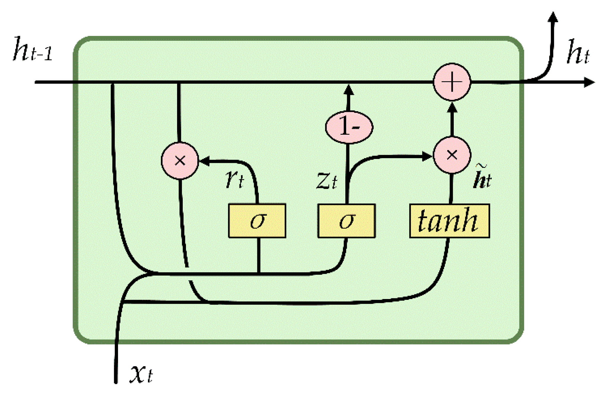
The gated recurrent unit cell architecture network (GRU) was proposed by Cho [31], which is a simplification of LSTM using update gate and reset gate to replace forget gate, input gate, and output gate. The structure diagram of GRU is as shown in Figure 8 [42].

In the structure of the gated recurrent unit cell, as shown in Figure 8, update equations are calculated as follows:

$${\mathrm{r}}_{\mathrm{t}}=\mathsf{\sigma }\left({\mathrm{W}}_{\mathrm{xr}}{\mathrm{x}}_{\mathrm{t}}{+\mathrm{W}}_{\mathrm{hr}}{\mathrm{h}}_{\mathrm{t}-1}{+\mathrm{b}}_{\mathrm{r}}\right)$$

(12)

$${\mathrm{z}}_{\mathrm{t}}=\mathsf{\sigma }\left({\mathrm{W}}_{\mathrm{xz}}{\mathrm{x}}_{\mathrm{t}}{+\mathrm{W}}_{\mathrm{hz}}{\mathrm{h}}_{\mathrm{t}-1}{+\mathrm{b}}_{\mathrm{z}}\right)$$

(13)

$$\widetilde{{\mathrm{c}}_{\mathrm{t}}}=\tan \mathrm{h}\left({\mathrm{W}}_{\mathrm{xc}}{\mathrm{x}}_{\mathrm{t}}{+\mathrm{W}}_{\mathrm{hc}}\left({\mathrm{r}}_{\mathrm{t}}{\ast \mathrm{h}}_{\mathrm{t}-1}\right){+\mathrm{b}}_{\mathrm{c}}\right)$$

(14)

$${\mathrm{c}}_{\mathrm{t}}=\left({1-\mathrm{z}}_{\mathrm{t}}\right){\ast \mathrm{c}}_{\mathrm{t}-1}{+\mathrm{z}}_{\mathrm{t}}\ast \widetilde{{\mathrm{c}}_{\mathrm{t}}}$$

(15)

$${\mathrm{h}}_{\mathrm{t}}{=\mathrm{c}}_{\mathrm{t}}$$

(16)

where r and z are the update gate and reset gate, respectively; W is the transformation weight matrix; b is the vector feature; x is the present input; σ is the activation function; and $\widetilde{c_t}$ is the output candidate value.

3.3. Accuracy Evaluation Measure

The evaluation of model accuracy is the dominant condition to measure the merits and disadvantages of the model. Since this paper studies numerical forecasts, it adopts the index to measure the regression model for evaluation. In this paper, four indicators are selected to evaluate the accuracy of the PM_2.5 concentration forecast, the R-square (R²), average absolute error (MAE), root mean square error (RMSE), and average absolute percentage error (MAPE). R² represents the goodness of fit of the deep learning model. When R² reaches 1, this model is the best deep learning model. RMSE is the square root of the mean square of the difference between the forecasted value and the observed value, which is used to measure the deviation between the forecasted value and the observed value. MAPE is the average value of the absolute value of the quotient of the difference between the forecasted value and the observed value, which is used to test the ratio of the forecasted error to the observed value. MAE is the relative error obtained by calculating the mean of the absolute value of the quotient of the difference between the predicted value and the observed value, which has powerful robustness to outliers. When the values of RMSE, MAPE, and MAE are smaller, the error of the forecast is smaller, and the accuracy of the model is higher. The calculation formula of the four evaluation indicators is shown in the following four Equations (17)–(20):

$${\mathrm{R}}^2=1-\frac{{{\displaystyle \sum }}_{\mathrm{i}=1}^{\mathrm{n}}{\left(\widehat{{\mathrm{y}}_{\mathrm{i}}}{-\mathrm{y}}_{\mathrm{i}}\right)}^2}{{{\displaystyle \sum }}_{\mathrm{i}=1}^{\mathrm{n}}{\left(\overline{{\mathrm{y}}_{\mathrm{i}}}{-\mathrm{y}}_{\mathrm{i}}\right)}^2}$$

(17)

$$\mathrm{RMSE}=\sqrt{\frac{1}{\mathrm{n}}{\displaystyle \sum }_{\mathrm{i}=1}^{\mathrm{n}}{\left(\widehat{{\mathrm{y}}_{\mathrm{i}}}{-\mathrm{y}}_{\mathrm{i}}\right)}^2}$$

(18)

$$\mathrm{MAPE}=\frac{100\%}{\mathrm{n}}{\displaystyle \sum }_{\mathrm{i}=1}^{\mathrm{n}}\left|\frac{\widehat{{\mathrm{y}}_{\mathrm{i}}}{-\mathrm{y}}_{\mathrm{i}}}{{\mathrm{y}}_{\mathrm{i}}}\right|$$

(19)

$$\mathrm{MAE}=\frac{1}{\mathrm{n}}{\displaystyle \sum }_{\mathrm{i}=1}^{\mathrm{n}}\left|\left(\widehat{{\mathrm{y}}_{\mathrm{i}}}{-\mathrm{y}}_{\mathrm{i}}\right)\right|$$

(20)

where y_i, $\widehat{y_i}$ and $\overline{y_i}$ represent the observed value, forecasted value and mean value of the PM_2.5 concentration, respectively; n refers to the total logarithm of data in the test set.

4. Experimental Results and Analysis

4.1. Experimental Setup

The CPU used in the experiment was an Intel Core i9 10900, the graphics card was RTX3080, and the operating system was a 64-bit Win10 system. All experiments were carried out under the above hardware and software conditions in this article, while also aiming at the same training set, validation set, and test set in different model experiments. We used four models to compare the differences between the models and to test the generalizability of our proposed method. These four models are random forests (RF), RNN, LSTM, and GRU. RF is a machine learning model designed under the scikit-learn framework, whereas the other three models are deep learning models. They are based on the PyTorch1.7.1+cu11.0 framework design, both of which are based on the Python programming language. In this article, we used the PM_2.5 concentration data of the first four hours combined with meteorological data, other pollutant data, and the PM_2.5 concentration data of nearby stations to forecast the PM_2.5 concentration value in the next hour [33]. The parameters of these deep learning models are shown in

Table 2. Parameter table of the deep learning model for PM_2.5 concentration forecasting.

Parameter	Value
Loss	MSE
Optimizer	Adam
Epochs	1000
Learning rate	0.001
Hidden size	40
Num layers	4
Input size	16

.

In deep learning, the optimizer is the most important model parameter required to establish the neural network in the PyTorch framework. The same as the study of Huang et al. [33], we selected the Adam optimization function as the optimizer for model training. We set the learning rate of these models to 0.001 and used the mean absolute error (MSE) to define the loss function. The recurrent neural network would achieve the best training effect when the MSE is reduced to a stable value. These experiments are carried out for a total of 1000 epochs. Finally, four evaluation indicators of R², RMSE, MAPE, and MAE were calculated to evaluate these models.

4.2. Results and Analysis

Table 3. Model performance of the proposed space diffuser and comparisons with other models.

Model	RNN		LSTM		GRU		RF
	Spatial RNN	Original RNN	Spatial LSTM	Original LSTM	Spatial GRU	Original GRU	Spatial RF	Original RF
MAE	5.521	6.478	4.881	5.523	5.210	5.834	5.106	7.041
RMSE	8.663	9.921	7.770	8.604	8.309	9.135	8.176	10.288
${\mathit{R}}^2$	0.914	0.887	0.931	0.915	0.921	0.904	0.923	0.879
MAPE	0.226	0.289	0.176	0.223	0.199	0.240	0.192	0.316

shows the experimental results of different methods, in which spatial RNN referred to the deep learning models combined with a spatial diffuser, whereas the original RNN referred to this model being just its original model. The other models were similar to the RNN. Table 3 lists the accuracy evaluation results of the RNN, LSTM, GRU, RF and their combination with spatial diffuser using MAE, RMSE, R², and MAPE.

Table 3 shows that regardless of whether the spatial diffuser was used, the evaluation indices of the deep learning models were better than those of the machine learning models. We can see that the evaluation indicators of the basic deep learning model RNN were superior to RF, and RNN’s MAE, RMSE, R², and MAPE were 6.478, 9.921, 0.887, and 0.289, respectively. These were better than that of the RF model’s respective 7.041, 10.288, 0.879, and 0.316, indicating that the deep learning model is more suitable to forecast PM_2.5 concentration value compared to the machine learning model. The forecasts had a higher goodness of fit and a smaller forecasting error.

Moreover, among all deep learning models, LSTM showed the best performance, with MAE, RMSE, R², and MAPE of 5.523, 8.604, 0.915, and 0.223, respectively, which was not only better than RNN’s respective 6.478, 9.921, 0.887, and 0.289; and GRU’s respective 5.834, 9.135, 0.904, and 0.240; but also, even better than those of the RNN model combined with the spatial diffuser, which were 5.521, 8.663, 0.914, and 0.226, respectively.

Most importantly, the RMSE, MAE, and MAPE of the models using the spatial diffuser were lower than those of the original models. The R² was closer to one, which indicates that the models using the spatial diffuser had a higher forecast accuracy and a better model fitting effect than with those not taking it into account. Compared with the original RNN, LSTM, GRU, and RF models, the proposed method exhibited decreases of 12.68%, 9.69%, 9.04%, and 20.53% in RMSE; 14.77%, 11.62%, 10.70%, and 27.48% in MAE; 21.80%, 20.08%, 17.08% and 39.24% in MAPE; and increases of 3.04%, 1.75%, 1.88%, and 5.01% in R², respectively. Then, among these models using the spatial diffuser, LSTM outperformed all other models, which were the RMSE, MAE, R2, and MAPE with values of 7.770, 4.881, 0.931, and 0.176, respectively. In summary, the LSTM model using the spatial diffuser had the least forecast bias and the best forecast effect among all of the models used in this paper.

Figure 9 shows the comparison results of the observed and forecasted values of PM_2.5 concentrations by using the proposed spatial diffuser. We found that for the forecast of high concentration of PM_2.5 concentration values, LSTM, GRU, and RF that used spatial diffusion can be more effectively detected, but RNN is not competent for this situation, and we can see that the data of the LSTM model combined with the spatial diffuser is closer to the diagonal line, indicating that the difference between the forecasted value and the measured value is the smallest. In summary, the LSTM model combined with the spatial diffuser achieved the best results in the PM_2.5 concentration forecast in the next hour.

5. Conclusions and Discussion

This paper proposes a spatial diffuser combined with PM_2.5 concentration data from nearby stations for PM_2.5 concentration forecasting in the central area of the Yangtze River Delta.

During the data analysis stage, it was found that according to the time series diagram, the PM_2.5 concentration characteristics were not visible and were difficult to capture. Therefore, we performed a comprehensive analysis of the factors that affect the change in PM_2.5 concentration. Most of the impact parameters were easily matched with PM_2.5 concentration data, but building a dataset that can describe the diffusion of pollutants was slightly complicated. Therefore, we designed a space diffuser to establish a dataset to match the PM_2.5 concentration data according to their spatial autocorrelation characteristics to enhance the potential to achieve better results for PM_2.5 concentration forecasting.

During the accuracy evaluation phase, first, for PM_2.5 concentration forecasting, the deep learning models proved to be meaningfully superior to the machine learning models, indicating that deep learning models can capture the time dependence of time series data effectively. This also makes them have a unique advantage in time series prediction. Moreover, among these deep learning models, LSTM has the highest prediction accuracy and the best goodness of fit in forecasting PM_2.5 concentration, which shows that LSTM has a better effect than RNN and GRU in forecasting PM_2.5 concentration in the central area of the Yangtze River Delta in the next hour by using data from the first 4 h. Most importantly, the forecast results are more accurate when provided with the dataset established by the spatial diffuser, regardless of whether deep learning models or machine learning models are employed, indicating that the expression of the gas diffusion process plays an important and positive role in the model forecast.

Although this spatial diffuser performs well, it still has some limitations that are associated with the method. First, there are some problems with the method of the correlation coefficient when selecting explanatory factors for forecasting PM_2.5 concentrations from alternative parameters. The correlation between the parameters and concentration does not imply the existence of causal relationships, and thus parameters with a high correlation coefficient but no causal relationship may be selected, increasing the time complexity. Moreover, according to the characteristics of the average atmospheric movement of 50 km per hour, we took the stations within 50 km as the adjacent stations, and then we forecast the PM_2.5 concentration one hour later. If multistep prediction is required, our model will need to be improved. At the same time, an increase in model parameters will inevitably lead to the increase in model complexity. In addition, using the spatial diffuser, we initially proposed to evaluate 167 stations in the study area; however, there were only 26 stations that met the data requirements. Therefore, we did not make forecasts for the remaining stations, which leads to a poor generalizability of our model. These problems will be taken into consideration in our subsequent research and theoretical implementation.

In the future, the method can be applied to other research areas and related forecasting problems after the corresponding adjustments and changes are made, such as forecasting the AQI and water pollution. Since air pollution is a serious health hazard, we can show the forecasting of hourly data in different locations of the municipality by the model for the benefit of the public.

References

1. Li, D.; Ma, J.; Cheng, T.; van Genderen, J.L.; Shao, Z. Challenges and opportunities for the development of MEGACITIES. Int. J. Digit. Earth 2018, 12, 1382–1395. [Google Scholar] [CrossRef]
2. Shao, Z.; Fu, H.; Li, D.; Altan, O.; Cheng, T. Remote sensing monitoring of multi-scale watersheds impermeability for urban hydrological evaluation. Remote Sens. Environ. 2019, 232, 111338. [Google Scholar] [CrossRef]
3. Xu, X.; Tong, T.; Zhang, W.; Meng, L. Fine-grained prediction of PM2.5 concentration based on multisource data and deep learning. Atmos. Pollut. Res. 2020, 11, 1728–1737. [Google Scholar] [CrossRef]
4. Spatial Variation of Multiple Air Pollutants and Their Potential Contributions to All-Cause, Respiratory, and Cardiovascular Mortality across China in 2015–2016. Available online: https://www.researchgate.net/publication/319575435_Spatial_variation_of_multiple_air_pollutants_and_their_potential_contributions_to_all-cause_respiratory_and_cardiovascular_mortality_across_China_in_2015-2016 (accessed on 17 October 2021).
5. Adipose Mesenchymal Stem Cell-Derived Antioxidative Extracellular Vesicles Exhibit Anti-Oxidative Stress and Immunomodulatory Effects under PM2.5 Exposure. Available online: https://www.researchgate.net/publication/347911247_Adipose_mesenchymal_stem_cell-derived_antioxidative_extracellular_vesicles_exhibit_anti-oxidative_stress_and_immunomodulatory_effects_under_PM25_exposure (accessed on 17 October 2021).
6. Ma, J.; Ding, Y.; Cheng, J.C.P.; Jiang, F.; Gan, V.J.L.; Xu, Z. A Lag-FLSTM deep learning network based on Bayesian Optimization for multi-sequential-variant PM2.5 prediction. Sustain. Cities Soc. 2020, 60, 102237. [Google Scholar] [CrossRef]
7. Zhang, Y.; Bocquet, M.; Mallet, V.; Seigneur, C.; Baklanov, A. Real-time air quality forecasting, part I: History, techniques, and current status. Atmos. Environ. 2012, 60, 632–655. [Google Scholar] [CrossRef]
8. Parrish, D.; Trainer, M.; Trivikrama Rao, S.; Solomon, P.A. Regional photochemical measurement and modeling studies conference San Diego, California 8–12 November 1993. Atmos. Environ. 1995, 29, 2885–2886. [Google Scholar] [CrossRef]
9. Wen, W.; Shen, S.; Liu, L.; Ma, X.; Wei, Y.; Wang, J.; Xing, Y.; Su, W. Comparative Analysis of PM2.5 and O3 Source in Beijing Using a Chemical Transport Model. Remote Sens. 2021, 13, 3457. [Google Scholar] [CrossRef]
10. Dou, C.; Ji, Z.; Xiao, Y.; Hu, Z.; Zhu, X.; Dong, W. Projection of Air Pollution in Northern China in the Two RCPs Scenarios. Remote Sens. 2021, 13, 3064. [Google Scholar] [CrossRef]
11. Vautard, R.; Builtjes, P.H.J.; Thunis, P.; Cuvelier, C.; Bedogni, M.; Bessagnet, B.; Honoré, C.; Moussiopoulos, N.; Pirovano, G.; Schaap, M.; et al. Evaluation and intercomparison of Ozone and PM10 simulations by several chemistry transport models over four European cities within the CityDelta project. Atmos. Environ. 2007, 41, 173–188. [Google Scholar] [CrossRef]
12. Jian, L.; Zhao, Y.; Zhu, Y.P.; Zhang, M.B.; Bertolatti, D. An application of ARIMA model to predict submicron particle concentrations from meteorological factors at a busy roadside in Hangzhou, China. Sci. Total Environ. 2012, 426, 336–345. [Google Scholar] [CrossRef]
13. Particulate Matter Air Quality Assessment Using Integrated Surface, Satellite, and Meteorological Products. Available online: https://www.researchgate.net/publication/252788692_Particulate_Matter_Air_Quality_Assessment_using_Integrated_Surface_Satellite_and_Meteorological_Products (accessed on 2 October 2021).
14. Davis, J.M.; Speckman, P. A model for predicting maximum and 8 h average ozone in Houston. Atmos. Environ. 1999, 33, 2487–2500. [Google Scholar] [CrossRef]
15. Hu, X.; Waller, L.A.; Al-Hamdan, M.Z.; Crosson, W.L.; Estes, M.G.; Estes, S.M.; Quattrochi, D.A.; Sarnat, J.A.; Liu, Y. Estimating ground-level PM2.5 concentrations in the southeastern U.S. using geographically weighted regression. Environ. Res. 2013, 121, 1–10. [Google Scholar] [CrossRef] [PubMed]
16. Sun, W.; Zhang, H.; Palazoglu, A.; Singh, A.; Zhang, W.; Liu, S. Prediction of 24-hour-average PM2.5 concentrations using a hidden Markov model with different emission distributions in Northern California. Sci. Total Environ. 2013, 443, 93–103. [Google Scholar] [CrossRef] [PubMed]
17. García Nieto, P.J.; Combarro, E.F.; Del Coz Díaz, J.J.; Montañés, E. A SVM-based regression model to study the air quality at local scale in Oviedo urban area (Northern Spain): A case study. Appl. Math. Comput. 2013, 219, 8923–8937. [Google Scholar] [CrossRef]
18. Chang-Hoi, H.; Park, I.; Oh, H.R.; Gim, H.J.; Hur, S.K.; Kim, J.; Choi, D.R. Development of a PM2.5 prediction model using a recurrent neural network algorithm for the Seoul metropolitan area, Republic of Korea. Atmos. Environ. 2021, 245, 118021. [Google Scholar] [CrossRef]
19. Laña, I.; Del Ser, J.; Padró, A.; Vélez, M.; Casanova-Mateo, C. The role of local urban traffic and meteorological conditions in air pollution: A data-based case study in Madrid, Spain. Atmos. Environ. 2016, 145, 424–438. [Google Scholar] [CrossRef]
20. Hooyberghs, J.; Mensink, C.; Dumont, G.; Fierens, F.; Brasseur, O. A neural network forecast for daily average PM10 concentrations in Belgium. Atmos. Environ. 2005, 39, 3279–3289. [Google Scholar] [CrossRef]
21. Kamińska, J.A. A random forest partition model for predicting NO2 concentrations from traffic flow and meteorological conditions. Sci. Total Environ. 2019, 651, 475–483. [Google Scholar] [CrossRef]
22. Shang, Z.; Deng, T.; He, J.; Duan, X. A novel model for hourly PM2.5 concentration prediction based on CART and EELM. Sci. Total Environ. 2019, 651, 3043–3052. [Google Scholar] [CrossRef]
23. Ma, X.; Tao, Z.; Wang, Y.; Yu, H.; Wang, Y. Long short-term memory neural network for traffic speed prediction using remote microwave sensor data. Transp. Res. Part C Emerg. Technol. 2015, 54, 187–197. [Google Scholar] [CrossRef]
24. Li, X.; Peng, L.; Hu, Y.; Shao, J.; Chi, T. Deep learning architecture for air quality predictions. Environ. Sci. Pollut. Res. 2016, 23, 22408–22417. [Google Scholar] [CrossRef] [PubMed]
25. Tian, H.; Zhao, Y.; Luo, M.; He, Q.; Han, Y.; Zeng, Z. Estimating PM2.5 from multisource data: A comparison of different machine learning models in the Pearl River Delta of China. Urban Clim. 2021, 35, 100740. [Google Scholar] [CrossRef]
26. Hochreiter, S.; Schmidhuber, J. Long Short-Term Memory. Neural Computation, 9, 1735–1780.—References—Scientific Research Publishing. Available online: https://www.scirp.org/reference/referencespapers.aspx?referenceid=2693822 (accessed on 2 October 2021).
27. Li, X.; Peng, L.; Yao, X.; Cui, S.; Hu, Y.; You, C.; Chi, T. Long short-term memory neural network for air pollutant concentration predictions: Method development and evaluation. Environ. Pollut. 2017, 231, 997–1004. [Google Scholar] [CrossRef]
28. Zhang, B.; Zhang, H.; Zhao, G.; Lian, J. Constructing a PM2.5 concentration prediction model by combining auto-encoder with Bi-LSTM neural networks. Environ. Model. Softw. 2020, 124, 104600. [Google Scholar] [CrossRef]
29. Chang, Y.S.; Chiao, H.T.; Abimannan, S.; Huang, Y.P.; Tsai, Y.T.; Lin, K.M. An LSTM-based aggregated model for air pollution forecasting. Atmos. Pollut. Res. 2020, 11, 1451–1463. [Google Scholar] [CrossRef]
30. Abirami, S.; Chitra, P. Regional air quality forecasting using spatiotemporal deep learning. J. Clean. Prod. 2021, 283, 125341. [Google Scholar] [CrossRef]
31. Chung, J.; Gulcehre, C.; Cho, K.; Bengio, Y. Empirical Evaluation of Gated Recurrent Neural Networks on Sequence Modeling. arXiv 2014, arXiv:1412.3555. [Google Scholar]
32. Tao, Q.; Liu, F.; Li, Y.; Sidorov, D. Air Pollution Forecasting Using a Deep Learning Model Based on 1D Convnets and Bidirectional GRU. IEEE Access 2019, 7, 76690–76698. [Google Scholar] [CrossRef]
33. Huang, G.; Li, X.; Zhang, B.; Ren, J. PM2.5 concentration forecasting at surface monitoring sites using GRU neural network based on empirical mode decomposition. Sci. Total Environ. 2021, 768, 144516. [Google Scholar] [CrossRef]
34. Pasquill, F.; Smith, F. Atmospheric Diffusion; E. Horwood: New York, NY, USA, 1983. [Google Scholar]
35. Chen, X.; Shao, S.; Tian, Z.; Xie, Z.; Yin, P. Impacts of air pollution and its spatial spillover effect on public health based on China’s big data sample. J. Clean. Prod. 2017, 142, 915–925. [Google Scholar] [CrossRef]
36. Li, X.; Wu, C.; Meadows, M.E.; Zhang, Z.; Lin, X.; Zhang, Z.; Chi, Y.; Feng, M.; Li, E.; Hu, Y. Factors Underlying Spatiotemporal Variations in Atmospheric PM2.5 Concentrations in Zhejiang Province, China. Remote Sens. 2021, 13, 3011. [Google Scholar] [CrossRef]
37. Pan, S.; Du, S.; Wang, X.; Zhang, X.; Xia, L.; Liu, J.; Pei, F.; Wei, Y. Analysis and interpretation of the particulate matter (PM10 and PM2.5) concentrations at the subway stations in Beijing, China. Sustain. Cities Soc. 2019, 45, 366–377. [Google Scholar] [CrossRef]
38. Pearson, K., VII. Note on regression and inheritance in the case of two parents. Proc. R. Soc. Lond. 1895, 58, 240–242. [Google Scholar] [CrossRef]
39. Huang, L.; Sun, J.; Jin, L.; Brown, N.J.; Hu, J. Strategies to reduce PM2.5 and O3 together during late summer and early fall in San Joaquin Valley, California. Atmos. Res. 2021, 258, 105633. [Google Scholar] [CrossRef]
40. Air Quality Designations for the 2012 PM-2.5 National Ambient Air Quality Standards Established. Available online: https://www.zhangqiaokeyan.com/academic-journal-foreign_air-pollution-consultant_thesis/0204110280407.html (accessed on 5 October 2021).
41. Sak, H.; Senior, A.; Beaufays, F. Long Short-Term Memory Based Recurrent Neural Network Architectures for Large Vocabulary Speech Recognition. arXiv 2014, arXiv:1402.1128. [Google Scholar]
42. Gao, S.; Huang, Y.; Zhang, S.; Han, J.; Wang, G.; Zhang, M.; Lin, Q. Short-term runoff prediction with GRU and LSTM networks without requiring time step optimization during sample generation. J. Hydrol. 2020, 589, 125188. [Google Scholar] [CrossRef]
Figure 1. Study area and the spatial distribution of ground monitoring stations.
Remotesensing 13 04834 g001
Figure 2. Map of the correlation coefficient between the PM2.5 concentration value and meteorological environment field data.
Remotesensing 13 04834 g002
Figure 3. Map of the correlation coefficient between the PM2.5 concentration value and all other pollutant parameters.
Remotesensing 13 04834 g003
Figure 4. Neighborhood partitioning and diffusion for Station S.
Remotesensing 13 04834 g004
Figure 5. Heatmap of the correlation coefficient between the central station and the surrounding stations.
Remotesensing 13 04834 g005
Figure 6. Recurrent neural network (RNN) architecture.
Remotesensing 13 04834 g006
Figure 7. Long short-term memory (LSTM) neural network.
Remotesensing 13 04834 g007
Figure 8. Gated recurrent unit (GRU) cell architecture.
Remotesensing 13 04834 g008
Figure 9. Comparisons of the forecasted PM2.5 concentration values with the measured PM2.5 concentration values.
Remotesensing 13 04834 g009