Article

Using Airborne Laser Scanning to Characterize Land-Use Systems in a Tropical Landscape Based on Vegetation Structural Metrics

1
Bioclimatology, Faculty of Forest Sciences, University of Goettingen, Büsgenweg 2, 37077 Göttingen, Germany
2
Silviculture of the Temperate Zone, Faculty of Forest Sciences, University of Goettingen, Büsgenweg 1, 37077 Göttingen, Germany
3
Functional Agrobiodiversity, University of Goettingen, Grisebachstr. 6, 37077 Göttingen, Germany
4
Faculty of Agriculture, Jambi University, Jl. Raya Jambi—Muara Bulian Km. 15, Mendalo Indah, Jambi Luar Kota, Jambi 36361, Indonesia
5
Chairs of Statistics and Econometrics, University of Goettingen, Humboldtallee 3, 37073 Göttingen, Germany
6
Faculty of Geo-Information Science and Earth Observation, University of Twente, Hengelosestraat 99, 7514AE Enschede, The Netherlands
7
Institute of Farm Economics, Thünen Institute, Bundesallee 63, 38116 Braunschweig, Germany
8
Centre of Biodiversity and Sustainable Land Use (CBL), University of Goettingen, Büsgenweg 1, 37077 Göttingen, Germany
*
Author to whom correspondence should be addressed.
Remote Sens. 2021, 13(23), 4794; https://doi.org/10.3390/rs13234794
Submission received: 11 October 2021 / Revised: 12 November 2021 / Accepted: 25 November 2021 / Published: 26 November 2021
(This article belongs to the Section Environmental Remote Sensing)

Abstract

:
Many Indonesian forests have been cleared and replaced by fast-growing cash crops (e.g., oil palm and rubber plantations), altering the vegetation structure of entire regions. Complex vegetation structure provides habitat niches to a large number of native species. Airborne laser scanning (ALS) can provide detailed three-dimensional information on vegetation structure. Here, we investigate the potential of ALS metrics to highlight differences across a gradient of land-use management intensities in Sumatra, Indonesia. We focused on tropical rainforests, jungle rubber, rubber plantations, oil palm plantations and transitional lands. Twenty-two ALS metrics were extracted from 183 plots. Analysis included a principal component analysis (PCA), analysis of variance (ANOVAs) and random forest (RF) characterization of the land use/land cover (LULC). Results from the PCA indicated that a greater number of canopy gaps are associated with oil palm plantations, while a taller stand height and higher vegetation structural metrics were linked with rainforest and jungle rubber. A clear separation in metrics performance between forest (including rainforest and jungle rubber) and oil palm was evident from the metrics pairwise comparison, with rubber plantations and transitional land behaving similar to forests (rainforest and jungle rubber) and oil palm plantations, according to different metrics. Lastly, two RF models were carried out: one using all five land uses (5LU), and one using four, merging jungle rubber with rainforest (4LU). The 5LU model resulted in a lower overall accuracy (51.1%) due to mismatches between jungle rubber and forest, while the 4LU model resulted in a higher accuracy (72.2%). Our results show the potential of ALS metrics to characterize different LULCs, which can be used to track changes in land use and their effect on ecosystem functioning, biodiversity and climate.

Graphical Abstract

1. Introduction

Land-use change and land degradation represent key contributors to the increase in greenhouse gas emissions, both globally [1] and in the tropics [2,3], while also having an important impact on the habitat quality for many native species [4]. In the period 2000–2018, an increase in the number and extent of large-scale land acquisitions (from both foreign and domestic investments) in the tropics has shown a predominance of permits granted for land-use changes through deforestation in favor of fast cash crops (e.g., oil palm and rubber plantations) [5], in addition to illegal land clearance by smallholders [6]. Moreover, among tropical countries, Indonesia has seen a rapid rate of primary forest loss (0.84 Mha/yr) due to land clearance for agricultural purposes [3] in the period 2000–2012. After the introduction of the moratorium policy in 2011, the rate of land conversion to plantations appears to have slowed down [7]. However, the impacts of these land-use changes on the vegetation structure of entire regions have not been investigated.
Vegetation structural complexity is considered a reliable proxy for ecosystem biodiversity and habitat quality, as it can provide insights into several ecosystem functions as well as their overall health [8,9,10,11]. Recently recognized as one of six Essential Biodiversity Variables (EBVs) [12], vegetation structural complexity depends on the dimensional, architectural and spatial patterns of plant individuals and increases with increasing heterogeneity of biomass distribution in the 3D space [13,14]. Vegetation structure is composed of different elements related to both the vertical and horizontal spatial arrangement of biomass [15], influencing and maintaining favorable microclimatic conditions for different biota [16,17,18]. It is commonly assumed that structurally complex vegetation provides high quality habitat for the dependent organisms [19,20], while less complex vegetation can have a high impact on the habitat selection of several mammal and bird species [21,22,23]. Tropical forests represent some of the most structurally complex, biodiverse and carbon-rich ecosystems on the planet [24,25], while also displaying a highly variable structural complexity across small spatial scales [26,27,28]. Transformed land-use systems—depending on their management intensity—might also hold important vegetation structural complexity and thus ecosystem functions. Therefore, it is of paramount importance to acquire detailed knowledge on the vegetation structural complexity of different land uses in a landscape for the effective management of highly modified tropical landscapes [29]. Measurements of structural complexity through traditional field surveys can be extremely costly and time consuming, particularly in remote areas in the tropics. Airborne or spaceborne remote sensing technologies can offer viable alternatives to traditional fieldwork, being more repeatable and less affected by human measurement errors [30].
Over the last few decades, the use of remote sensing has gained much popularity in the fields of forestry and ecology, often playing a key role in providing a monitoring baseline for spatiotemporal changes in vegetation health and forest cover [30,31,32,33]. Among remote sensing technologies, light detection and ranging (LiDAR—also referred to as airborne laser scanning (ALS) when mounted on an airplane) is likely the most suited system to study vegetation structure (and structural complexity), due to the nature of the active sensor and its signal propagation and measurement, which can penetrate the canopy layer and provide insight on the elements below it. LiDAR-derived information can allow the precise estimation of several key vegetation structural attributes [30]: quantification of plot-level gap fraction, gap sizes and distribution [34,35]; maximum tree height and aboveground biomass (AGB) [36]; and leaf-area index (LAI) for any given vertical foliage profile contained within a plot [37]. Furthermore, over the last decade, several studies have tried to estimate vegetation structure through the use of LiDAR technology at different scales [38,39,40]. Using discrete return ALS data, authors were able to map regional variations in vegetation structural complexity over a large part of the Canadian province of Alberta [39]. In their study, Guo et al. [41], using six variables derived from LiDAR (i.e., standard deviation of heights, canopy cover and four measures of canopy height density), were able to significantly differentiate between eight different vegetation structural classes distributed across nine natural subregions. Moreover, Marselis et al. [42] were recently able to characterize five different vegetation types in a tropical forest–savanna mosaic across a large portion of Gabon, Africa. Recently, through the use of LiDAR data, Davies et al. [21] have found that on the island of Borneo, orangutan individuals were more likely to move through forests characterized by an increased canopy closure and by a tall, uniform vegetation layer, while they preferred avoiding canopy gaps. Using remote sensing measurements of forest structure, another study on Bornean forests showed that several mammal species were particularly sensitive to structural simplification after forest disturbance (e.g., repeated logging—[43]). Other studies have found that the presence of agricultural or urbanized land covers generally reduces the abundance and diversity of stingless bees in Thailand [44]. Barnes et al. [45] found that species richness of invertebrate detritivores in Sumatra was significantly lower in highly modified cash-crop monocultures (e.g., rubber and oil palm plantations), rather than in forested ecosystems. Indeed, vegetation structure can also affect arthropod species richness and their relative abundance, depending on the species composition and related leaf quality and distribution for herbivorous species [46]. However, to date, few studies have focused on the vegetation structural characterization of different land uses using LiDAR data in highly fragmented and modified tropical regions, such as the Indonesian island of Sumatra.
Here we aim to study the potential of ALS-derived measures to highlight differences in tropical vegetation structure from plots sampled across a gradient of land-use management intensity on the island of Sumatra, Indonesia. For this purpose, we analyzed the vegetation structure of five land uses of relevance in the region: tropical rainforests, jungle rubber, rubber plantations, oil palm plantations and transitional lands. Particularly, we (i) investigated the possible directionalities of the derived LiDAR metrics using a principal component analysis (PCA); (ii) focused on the behavior of key structural metrics across the different LULCs, by carrying out analysis of variance (ANOVA) and post-hoc pairwise comparisons; and (iii) trained a random forest (RF) classification algorithm to further characterize the target LULCs. Since we anticipate that the inclusion of both tropical rainforest and jungle rubber plots will result in a lower classification accuracy (due to their similar vegetation structural properties—[47]), two separate RF characterizations were carried out, one including all five LULCs (hereafter referred to as the “five land uses” (5LU) model) and one using only four LULCs (hereafter referred to as the “four land uses” (4LU) model), with the forest class being represented by a combination of plots belonging to both forest and jungle rubber classes.

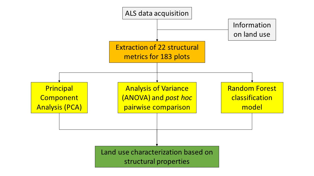
2. Materials and Methods
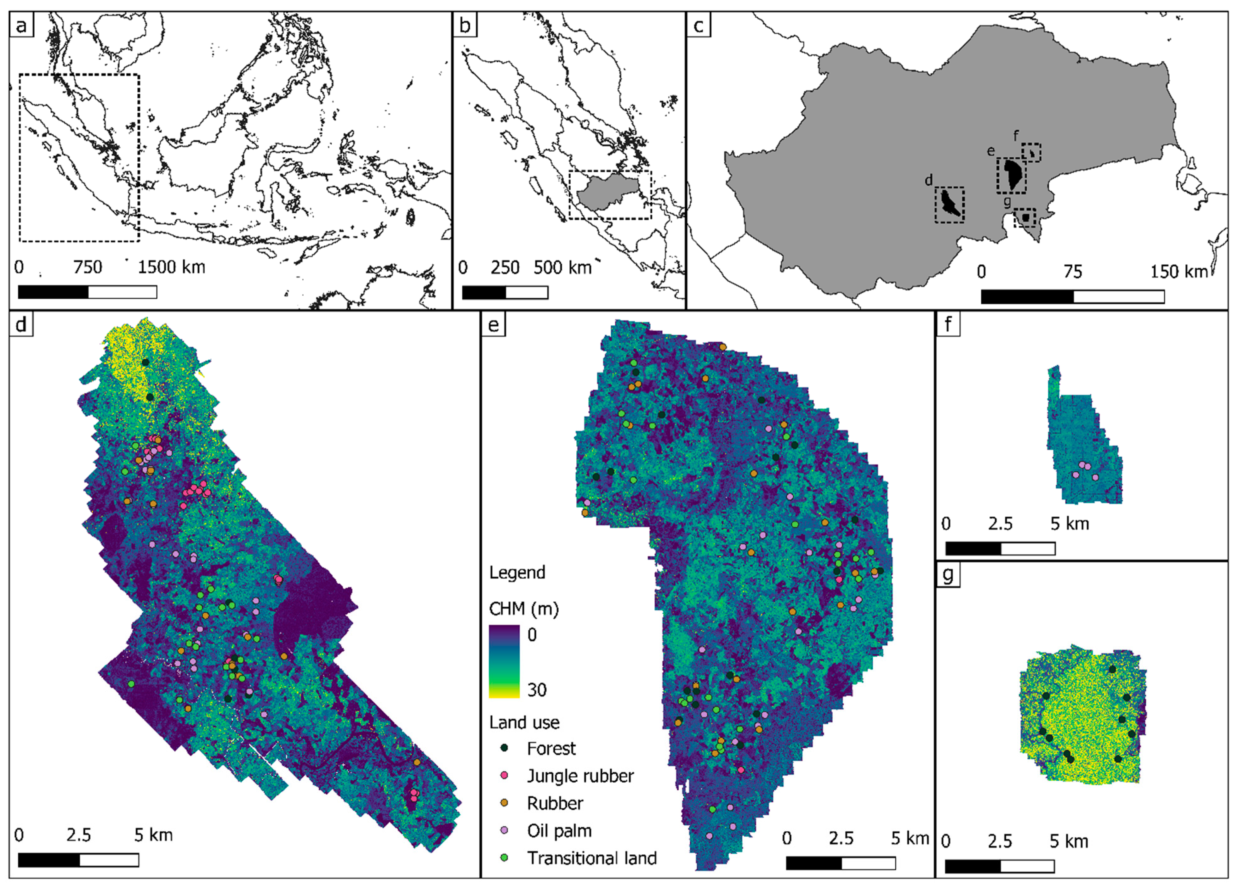
2.1. Study Area

This study is part of the Collaborative Research Centre 990: Ecological and Socioeconomic Functions of Tropical Lowland Rainforest Transformation Systems (CRC990: EFForTS project, https://www.uni-goettingen.de/efforts, accessed on 15 November 2021), located in Jambi Province, on the island of Sumatra, Indonesia (Figure 1a–c). Jambi province is characterized by lowlands stretching from the Barisan mountain range on the west to the southern Malacca Strait on the east. The province covers a total land surface of 50,160 km2 (Figure 1c), with a tropical humid climate characterized by 2235 ± 381 mm of mean annual precipitations and by an average annual temperature of 26.7 ± 0.2 °C [48]. Through history, the province’s rainforests have regularly been harvested for timber and non-woody products [49,50]. In many occasions, previously logged rainforests were also further modified by the inclusion of rubber trees, resulting in a mosaic of small-holder agroforestry systems, referred to as jungle rubber [51]. Over the past 50 years, in an effort to improve the province’s economic development, the Indonesian government has been releasing commercial logging concessions as well as supporting migration schemes from densely populated areas [52,53]. This has resulted in a rapid land-use change, with a continuous decrease in the extent of rainforests. By 2013, rainforests covered only 30% of the province, with forests located mainly in mountainous or protected areas. On the other hand, agricultural areas accounted for up to 55% of the land, with approximately 10% of degraded or fallow land (mainly waiting for monoculture conversion) [48]. As of 2014, more than 5900 km2 of oil palm and more than 6500 km2 of rubber were cultivated in Jambi Province, accounting alone for 12% and 13% or the total province cover, respectively [54].
For the purposes of this study, five land-use and land-cover (LULC) classes were considered (Figure 2): tropical rainforest; jungle rubber; rubber plantations; oil palm plantations; and transitional lands. These five LULC classes are defined as follows:
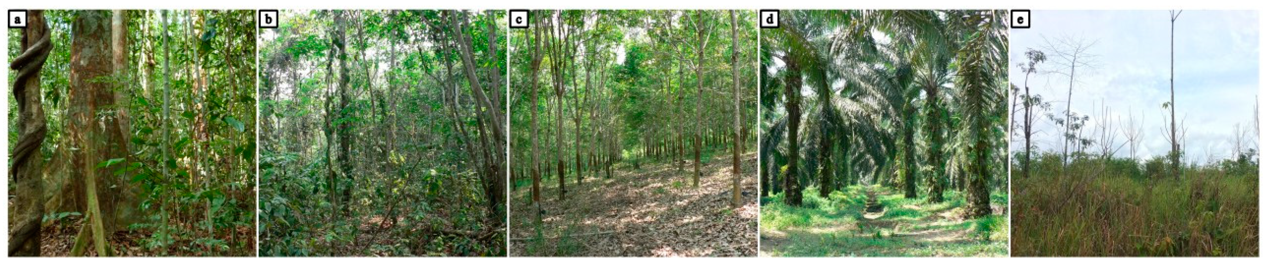
  • Tropical rainforest—areas dominated by trees (mainly including secondary rainforests as well as primary degraded rainforests), containing a minimum of 50% tree canopy closure above the lowest vegetation layer (to exclude tall, closed canopy transitional lands);
  • Jungle rubber—rubber trees (Hevea brasiliensis) scattered in the jungle, with as little as 10% rubber tree stems out of the total stem number in a 2500 m2 area;
  • Rubber plantation—regular plantation monocultures of rubber trees;
  • Oil palm plantation—any oil palm (Elaeis guineensis) monoculture, including intercropped and uneven-aged stands;
  • Transitional land (shrubland)—unused fallow land, including grasslands, which are in transition to secondary forest or cleared for plantation, containing up to 50% tree canopy closure above the lowest vegetation layer.
A total of 183 plots were available, following an opportunistic sampling design (i.e., using land-use information on all available plots falling within the LiDAR data coverage), deriving from different phases of the EFForTS project (visual inspection of each plot was carried out using the LiDAR data to ensure the information on the land use was still up to date). Among them, the five LULC classes investigated had the following representation: 34 plots of tropical secondary rainforest, 28 of jungle rubber, 36 of rubber plantation, 48 of oil palm plantation and 37 of transitional land. Plot locations ranged from the state-owned oil palm plantation PTPN 6 (Figure 1f), part of the Batanghari regency (Figure 1e), as well as within the Harapan rainforest protected area (Figure 1g) and within the Sarolangun regency (Figure 1d). Each circular plot covered an area of 1000 m2 (i.e., radius = 17.84 m).

2.2. ALS Data Acquisition and Pre-Processing

ALS data were collected on seven separate days between 24 January and 5 February 2020, over four study areas covering a total surface of 434,14 km2 (Figure 1c). The flying days were not consecutive due to bad weather conditions over the survey area. The acquisition flights were carried out using a BN2T fixed-wing aircraft based in Jambi, at an altitude up to 15,500 ft above ground level (AGL). LiDAR data were collected using a Riegl LMS-Q780 full waveform scanner (Riegl Laser Measurement Systems GmbH, Horn, Austria), operating at the near-infrared wavelength. The sensor has a wide field of view of 60° (+/−30° from nadir), and a high laser pulse repetition rate of up to 400 kHz. The ALS acquisitions were collected and processed by Dimap HK Pty Limited (Kowloon, Hong Kong). The final point cloud density varied within and between study areas, with mean point densities ranging from 16.6 points m−2 to 40.5 points m−2. The canopy height models (CHMs) at 1 m resolution were obtained through the subtraction of DSM and DTM in ArcGIS Pro (ESRI, Redlands, CA, USA), using the raster calculator.

2.3. Metrics Extraction and Calculation

The extraction and computation of all but one (see below) vegetation structural metric at the plot level were undertaken in the statistical language R, version 4.0.0 [55]. Individual point clouds (for each of the 183 plots) were clipped out of the height-normalized (i.e., height of the points relative to the ground) LiDAR dataset using the “lasclip()” function of the lidR package [56]. For each individual plot, a suite of ALS-derived metrics was computed (see Table 1). These metrics included a mix of different variables quantifying different aspects of vegetation structure and were selected due to their wide implementation in the literature, as well as their relative ease-of-computation (related to readily available R packages): traditional stand summary measures (e.g., maximum stand height, vegetation cover, LAI, total gap area); complexity/heterogeneity measures (e.g., box-dimension (Db), height entropy and kurtosis, rumple index); measures of vertical structure (e.g., height percentiles within the stand, effective number of layers (ENL), foliage height diversity (FHD), canopy ratio (CR)); and measures of horizontal structure (e.g., number of canopy gaps, gap area statistics). Forest gaps (Figure 3) were defined as areas within the forest canopy where the tallest top of the crown of any stem was noticeably lower than the crown height of the surrounding trees [57]. LiDAR summary statistics represent the most commonly used metrics in remote sensing forest inventory studies [58,59,60], and were therefore included in our selection of descriptive metrics. Additionally, several metrics related to vegetation structure, depicting the layering of vegetation elements (i.e., lai, enl, fhd_shan_eve and fhd_shan_divTable 1), space occupancy (i.e., DbTable 1) and top of the crown surface complexity (i.e., rumpleTable 1), were included as they are important indicators of habitat quality [46,61]. Lastly, as mentioned above, information on the size and distribution of the canopy gaps in the horizontal vegetation layer is important, as it can influence the behavior and movement of several different animals [21]. Forest gaps were quantified using the “GapStats()” function, which requires the setting of a minimum gap height threshold, defined as the minimum height underneath which no remaining trees could be identified [62]. In the present study, given the nature of the vegetation found in the five land uses, this minimum height threshold was set to 2.5 m, to avoid the inclusion of the shrub layer as part of the canopy.

2.4. Statistical Analysis

All statistical analyses were carried out in R statistical software version 4.0.0 [55].

2.4.1. Principal Component Analysis (PCA)

To examine whether possible directionalities of the derived LiDAR metrics could help characterize different land-use types, a principal component analysis (PCA) was undertaken [69,70]. A first characterization of the variation in component composition of the different LULCs was carried out through PCA, by capturing the maximum variance in a finite number of orthogonal components on the basis of an eigenvector analysis of the covariance matrix data [71]. The PCA analysis was computed using the “PCA()” function from the FactoMineR package [72]. PCA results were graphically visualized as a biplot, showing both the directionality of the LiDAR metrics as well as the distribution of sampled points, using the “fviz_pca_biplot()” function from the factoextra package [73].

2.4.2. Analysis of Variance (ANOVA) and Post-Hoc Pairwise Comparison

To investigate differences in the 22 LiDAR-derived metrics between the different land uses a one-way analysis of variance (ANOVA—“aov()” function of the stats package) was used [74]. The assumptions of normality of the residuals and homoscedasticity were tested using the Shapiro–Wilk test [75] (“shapiro.test()” function of the stats package) and Levene’s test [76] (“leveneTest()” of the car package), respectively. When the normality assumption was not met, the Kruskal–Wallis non-parametric test [77] (“kruskal.test()” from the stats package) was used instead to analyze the structural metrics. When only the assumption of normality was met but not that of homoscedasticity, Welch-ANOVA (“welch_anova_test()” from the rstatix package) was used, following Shingala and Rajyaguru [78]. Significant differences of each metric among the five LULCs were then investigated with a post-hoc pairwise comparison analysis, by carrying out either the Tukey test (“TukeyHSD()” from the stats) for ANOVA, the Dunn test (“DunnTest()” from the DescTools package—[79]) for the Kruskal–Wallis test or the Games–Howell test (“games_howell_test” from the rstatix package) for the Welch-ANOVA [78,80]. In all cases, post-hoc test results with a p-value < 0.1 were deemed significant.

2.4.3. Random Forest Land-Use Characterization

To further characterize the different land uses, a classification of different LULCs was performed using the non-parametric ensemble learning algorithm random forest (RF—[81]), executed using the extendedForest package [82]. Random forest firstly creates a random bootstrapped subsample of the training data for a single classification tree, where two-thirds of the data are used to build the tree. Within the tree, each node is split based on a restricted subset of predictor variables. The accuracy relative to each tree is then calculated using the data not contained within the bootstrapped subsample, which is termed the out-of-bag (OOB) sample. Since the OOB sample is withheld from the procedure of tree growing, the OOB estimate can be essentially considered equivalent to a leave-one-out cross validation [83]. This procedure was repeated to grow classification trees to minimize the OOB estimate of error rate and to avoid overfitting the training data [83,84]. Since many of the LiDAR-derived metrics used here were strongly correlated with each other (see Figure A1), the extendedForest variant of RF was used. extendedForest implements a conditional permutation method proposed by Strobl et al. [85] to account for biased variable importance selection due to the intercorrelation among predictor variables, since a strong correlation between predictor variables can inflate the importance of each variable [81]. Random forest requires two parameters to be manually input (i.e., ntree and mtry), which here were set to 100 and 3, respectively. The choice of the value of number of trees ntree and mtry was made to minimize the OOB error rate. In the present case, first we implemented a model (i.e., 5LU model) to classify the five different land uses as a function of the metrics extracted from the LiDAR data. Overall, 140 plots out of the total 183 plots available were included in this model, with each land-use class represented by 28 plots (i.e., the maximum number of plots in the least represented category—jungle rubber). Prior to model fitting, the dataset was randomly stratified with respect to the grouping factor (i.e., land use) into a training (2/3–95 plots (19 plots per LULC)) and validation (1/3–45 plots (9 plots per LULC)) dataset, where both the training and validation datasets had a balanced sample size with respect to the grouping factor. This was done to avoid any potential bias deriving from imbalanced training and validation datasets. The same procedure was then repeated, but in this instance, the classification algorithm was targeting only four land uses (i.e., 4LU model), using a novel forest class obtained from the combination of 14 randomly selected plots from the forest plots and 14 from the jungle rubber plots (as we posit that no evident structural differences would be found between the two land uses [47], thus greatly reducing the classification accuracy of our 5LU model). This resulted in the utilization of 112 plots, once again randomly partitioned into training (2/3–76 plots) and validation (1/3–36 plots) datasets.
The importance of each LiDAR predictor variable in the fitted RF model was evaluated using the mean decrease in accuracy (MDA–[86]), computed with the “importance()” function within the extendedForest package [82]. Higher MDA values correspond to predictor variables important for the differentiation of land uses. After fitting a preliminary model, predictor variables with a negative MDA in the overall model were removed following Costa e Silva et al. [87]. The model was then re-fitted with the retained variables to produce the final classification model. To assess the ability of the fitted RF model to predict the different land uses, four measures of accuracy and model fit were calculated from the independent validation dataset following Congalton [88], using the confusion matrix from the RF model and the fmsb package [89]. These measures included (i) overall accuracy (OA), denoting the probability that a randomly selected element (e.g., a survey plot) has been correctly classified, obtained as the sum of elements correctly classified (i.e., true positive) divided by the total number of elements (i.e., total number of plots); (ii) producer’s accuracy (PA), computed as the proportion between the total number of correctly classified elements within each class and the total number of elements in that class; (iii) user’s accuracy (UA), calculated by dividing the number of elements correctly classified in each class and the total number of elements classified to that class (i.e., true positive plus false positive); and (iv) Cohen’s Kappa coefficient, which is confined between values from 0 to 1 (i.e., 0 indicates poor agreement between the predicted classification and ground-truth, while 1 indicates perfect agreement), and quantifies the reproducibility of a discrete variable by measuring the difference between the observed accuracy and that expected through chance alone [90].

3. Results

3.1. Principal Component Analysis (PCA)

The overall variation across the 22 LiDAR-derived metrics is summarized by the principal component analysis (Figure 4). Table 2 lists the eigenvalues of the LiDAR-derived metrics with the first four components identified. The first two principal components (PC1 and PC2 shown in Figure 4) accounted for 64% and 14.7% of the total variance among samples, while PC3 and PC4 only accounted for 8.1% and 3.3%, respectively. The main variation was due to the independent variation in the levels of the four main groups of metrics. The first group comprised 14 metrics mainly related to stand summary statistics (i.e., zmax and lai), measures of vertical structure (i.e., pzabove2, zq25, zq50, zq75, fhd_shan_div, fhd_shan_eve, en and Dbl) and measure of complexity/heterogeneity (i.e., zsd, zentropy and rumple). From the scatter plot representation of the different plots studied here, the first group of metrics seemed to guide the grouping of mainly forest, jungle rubber and taller rubber plantation plots (Figure 4). The second group, which almost completely identified with the second component (PC2 in Figure 4 and Table 2), was represented by the num_gaps metric. This seemed to be mostly related to the presence of oil palm plots (Figure 4). The third and fourth groups were represented by the cr metric (diagonal to the two principal components), and by zskew, zkurt and metrics of horizontal structure (i.e., min_gapArea, mean_gapArea, max_gapArea and sum_gapArea), respectively (Figure 4). All of these were mainly related with the occurrence of oil palm plantations (cr) and with transitional lands (zskew, zkurt and horizontal structure metrics).

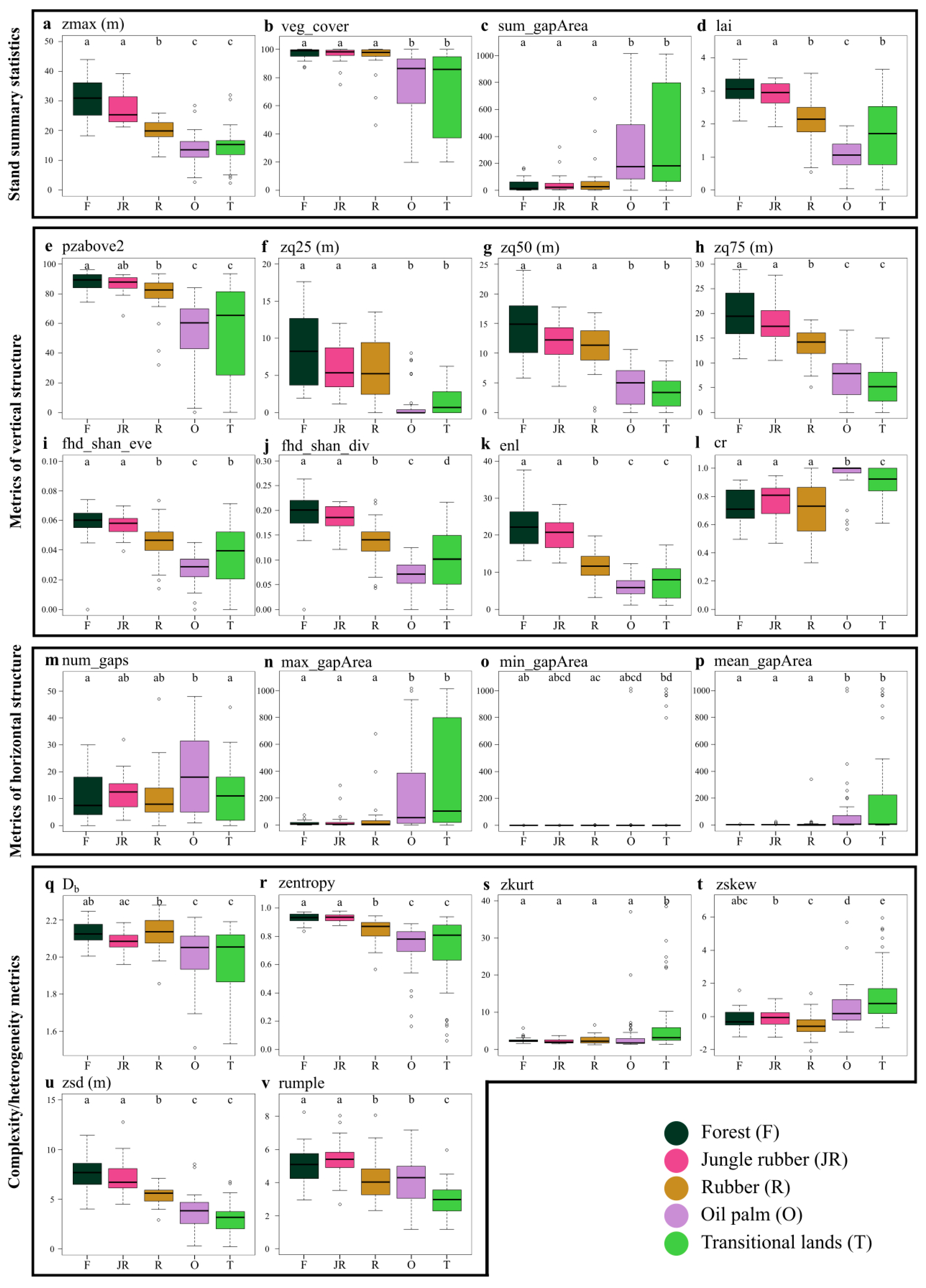
3.2. Analysis of Variance (ANOVA) and Post-Hoc Pairwise Comparison

Results from the analysis of variance and the subsequent post-hoc pairwise comparison of the means of the population values of all the LiDAR metrics are presented in Figure 5. Of the 22 metrics investigated, only rumple met the ANOVA assumptions of normality of the residuals and homoscedasticity and was therefore tested with a one-way ANOVA and Tukey test (Figure 5v). The residuals of zsd were also normally distributed, but the assumption of homoscedasticity was not met, and thus it was tested using a Welch-ANOVA and the Games–Howell post-hoc pairwise comparison. All other metrics were tested with the non-parametric Kruskal–Wallis test and their post-hoc pairwise comparisons were carried out using the Dunn test (see Section 2.4.2). A total of 20 of the 22 metrics behaved significantly different at the p < 0.001 level across the different land uses, with differences in min_gapArea and num_gaps being significant at the p < 0.01 and p < 0.05 levels, respectively. From the post-hoc pairwise comparisons, no significant differences were found in any metric between the forest and jungle rubber plots (Figure 5). With the exception of zkurt and min_gapArea, all other metrics showed significantly different behaviors between forest and oil palm plots. Significant differences were also identified in most traits between jungle rubber and oil palm plots, with a few exceptions (i.e., num_gaps, min_gapArea, Db and zkurt—see Figure 5m,o,q,s). On one hand, when looking at the rubber plantation plots, several metrics (i.e., zmax, zsd, zskew, zentropy, zq75, lai, fhd_shan_div, fhd_shan_eve and enl) showed an intermediate behavior between the forested plots (including both forest and jungle rubber plots) and oil palm and transitional plots (Figure 5). On the other hand, other LiDAR metrics were not significantly different between the rubber plantations and forest plots (i.e., zskew and Db), jungle rubber plots (i.e., pzabove2 and num_gaps) and forest and jungle rubber plots (i.e., zkurt, zq25, zq50, cr, veg_cover and all the gaps analysis summary statistics, except for num_gaps). Transitional land plots were significantly different from the other LULCs with respect to zskew, zkurt, rumple, fhd_shan_div and cr, while they showed no significant differences from oil palm plots in all metrics except for lai, fhd_shan_eve and num_gaps (Figure 5d,i,m).

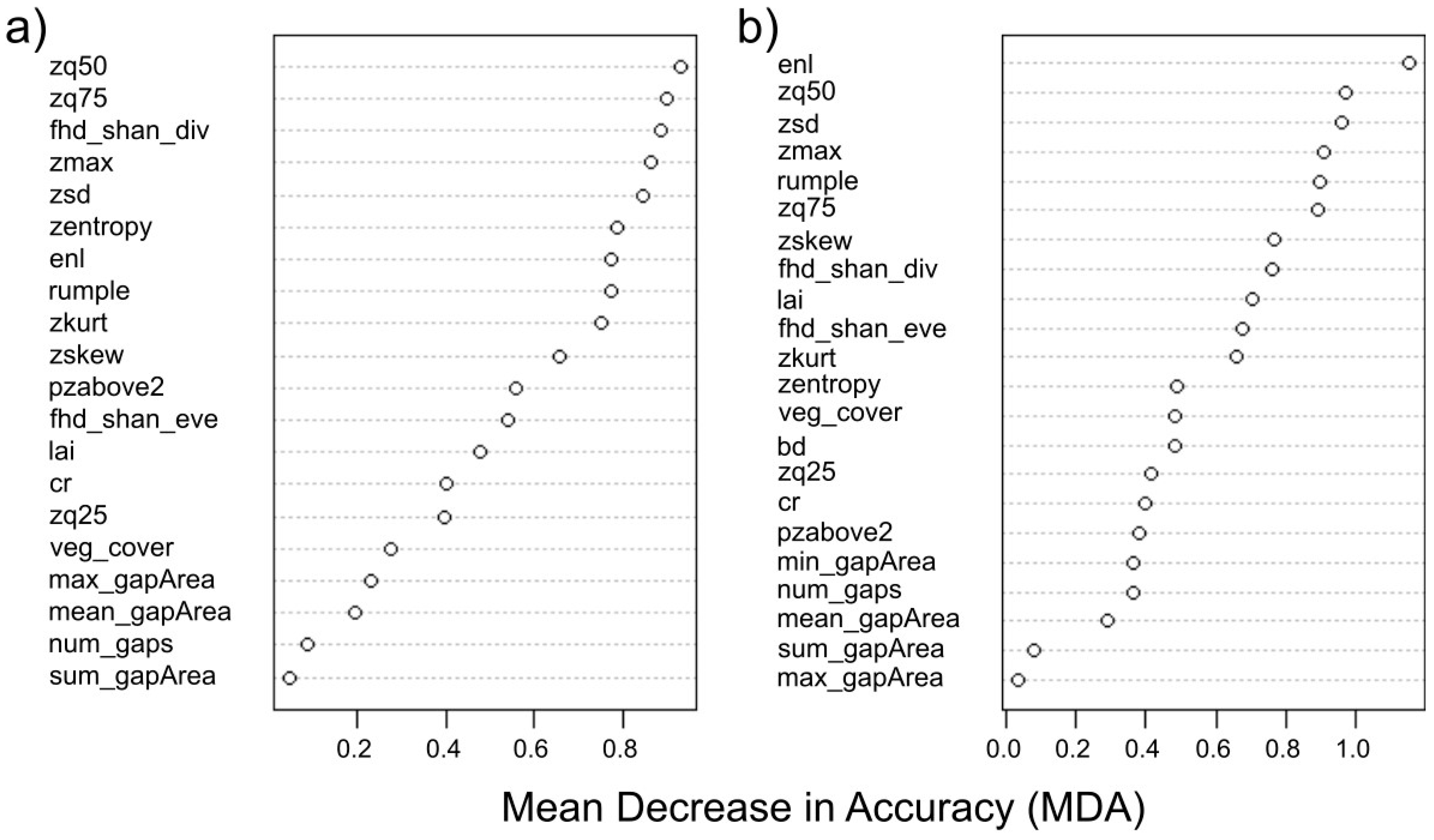
3.3. Random Forest Land-Use Characterizations

The OOB error rate amounted to 37.9% for the 5LU model and to 32.9% for the 4LU model. The 5LU model resulted in an overall accuracy and Cohen’s kappa of 51.1% and 0.39, respectively (Table 3). The 4LU model returned a higher overall accuracy (72.2%) and Cohen’s kappa (0.63) values (Table 4). Values of user’s accuracy from the 5LU model remained centered around the 50% mark (forest and oil palm), with jungle rubber and rubber plots performing slightly better and transitional lands performing the worst (Table 3). Producer’s accuracies for the 5LU model varied widely, with oil palm plots performing the worst and transitional land plots performing the best (Table 3). When looking at the results from the 4LU model, almost all the producer’s and user’s accuracy values increased from the values obtained for the 5LU model (with the exception of user’s accuracy for rubber plots), with values ranging between 44.4% and 100% in user’s accuracy, and between 60.0% and 100.0% in producer’s accuracy (Table 4). Figure 6 shows the mean decreases in accuracy (MDA) for all the metrics included in the two RF models (i.e., 5LU and 4LU). Only in the case of the 5LU model two metrics were removed (i.e., min_gapArea and Db), as they showed negative MDA values in the preliminary model (see Section 2.4.3). The top five most important metrics for the 5LU model were zq50, zq75, fhd_shan_div, zmax and zsd (Figure 6a). Other measures followed without a particular order, gradually decreasing their relative importance in the model, with metrics of horizontal structure having the lowest values of MDA (Figure 6a). The most important metrics for the 4LU model were enl, zq50, zsd, zmax and rumple (Figure 6b). Although following a different order, also in this case the more important metrics belonged to metrics of vertical structure and complexity/heterogeneity metrics, with metrics of horizontal structure ranking among the least important (Figure 6b). Table 5 and Table 6 report all the values of a mean decrease in accuracy (MDA) associated with each LiDAR-derived metric and LULC, used in the 5LU model and in the 4LU model, respectively.
When looking at the results from the 5LU model, metrics related to measures of height distribution, height description and vegetation structural indices were among the most important when classifying forest plots, with metrics related to gap analysis ranking the least important (mean_gapArea, veg_cover and sum_gapArea even displaying negative importance—Table 5). In agreement with the PCA and ANOVA results, a similar trend to that identified for the forest class was also found for the jungle rubber class (i.e., height measures and structural indices were more important than metrics of horizontal structure—Table 5). The remaining LULC classes had a more variable distribution of important metrics, with measures related to gaps occurrence ranking the fourth from the top for rubber (i.e., veg_cover), while also having negative importance values in other classes (Table 5). Of all the land-use classes, transitional land had the highest number of metrics, showing negative importance (n = 5), with structural indices representing most of these metrics (4 out of 5—Table 5).
Alternatively, when focusing on the MDA results for the 4LU model, the order of importance of metrics changed quite noticeably, with enl being the most important metric for both forest (i.e., the novel forest class resulting from the balanced random merge of plots from forest and jungle rubber classes) and rubber classes (Table 6). Measures of height and height distribution ranked among the most important across all four land uses, but interestingly, rumple ranked as the second most important metric for transitional lands (Table 6). Furthermore, contrary to the results obtained from the forest and jungle rubber classes of the 5LU model, not all metrics related to the gap analysis rank lowest for the novel forest class. Additionally, these metrics showed reasonably high importance values for the transitional land class, which is in agreement with the results from the PCA (Table 6).

4. Discussions

The results of both the PCA and individual metrics analysis of variance helped in characterizing the five land uses under study, according to differences in the behavior of the LiDAR-derived metrics. The first component identified by the PCA (i.e., PC1 in Figure 4) was strongly associated (eigenvalues > 0.85) with metrics related to tall vegetation occurrence (i.e., pzabove2, zq75, zq50), entropy of height points (i.e., zentropy), vegetation layering (i.e., fhd_shan_div, lai and fhd_shan_eve) and horizontal spatial occupation of elements (i.e., veg_cover, sum_gapArea and max_gapArea). Indeed, plots distributed along this dimension followed a clear pattern: moving from transitional land to oil palm, rubber, jungle rubber and forest plots, going from negative to positive values of the first component. This trend is easily explainable when considering the post-hoc pairwise comparisons of most metrics, as the different land uses seem to exhibit a clear pattern following a decreasing gradient in land-use management intensity: from highly degraded (i.e., transitional lands) and strongly managed land uses (i.e., oil palm and rubber plantations) to less managed (i.e., jungle rubber) and relatively unmanaged (i.e., secondary rainforest) land uses.
Rainforests and jungle rubber plots tended to have taller and more complex vegetation, followed by rubber and the remaining land uses (Figure 5a,d,i–k,v). This trend agrees with the plots distributed along the positive axis of the first component, while plots mainly belonging to the transitional land and oil palm classes (and a few rubber plantation plots) were distributed along the negative axis. Moreover, measures of height skewness and kurtosis, as well as horizontal structure tended to be significantly higher for plots of transitional land (Figure 5c,m–p,s,t), which is possibly due to the higher variability in vegetation conditions displayed by these plots and typical of this vegetation type [91]. These trends are consistent with those identified in a recent study estimating carbon storage on a subset of these plots, where rainforest had the highest values of aboveground carbon storage (of which stand canopy height is a proxy), followed by rubber and oil palm monoculture [92].
When focusing on the second component identified by the PCA (i.e., PC2 in Figure 4) the distribution of plots appears to become less defined. Indeed, this component strongly identified with the num_gaps metric (Table 2, PC2), with several oil palm plots located towards the higher negative values of it. This could indicate that a higher number of gaps in the vegetation canopy could be indicative of oil palm plots, which are indeed characterized by a highly regular planting pattern [93,94]. This planting pattern creates gaps in the surroundings of each oil palm tree, at least until the plantation age reaches maturity, by which time the canopy will be mostly closed. This trend was further confirmed by the post-hoc pairwise analysis of the num_gaps metric, as the number of gaps in oil palm plots was significantly higher than those in forest and transitional land plots, and double the values obtained for jungle rubber and rubber plantation plots (Figure 5m). Interestingly, when looking at the results obtained from the 5LU RF model, the num_gaps metric was actually one of the two metrics dropped from the model, as it had a negative MDA value in the preliminary model. This was not the case for the 4LU RF model; nevertheless, num_gaps was the fourth least important metric in that model (Figure 6b).
Results from the post-hoc pairwise analysis of variance showed that no metric performed significantly different for all land uses considered, with forest and jungle rubber plots never showing significant differences between them. While forest and oil palm plots differed significantly for most metrics tested (with the exclusion of zkurt and min_gapArea), rubber plantation and transitional land plots performed differently according to different LiDAR-derived metrics (Figure 5). Rubber plantation plots did not show significant differences from forest and jungle rubber plots for zkurt, zq25, zq50, cr and for all metrics of horizontal structure, and they performed similar to oil palm plots in the case of rumple, min_gapArea and num_gaps. This could be due to the regular planting patterns employed in both oil palm and rubber plantations, which might have resulted in similar values for these metrics. Indeed, as the rumple index is mostly depended on the surface complexity of the top layer of the vegetation canopy [66], regularly alternating crowns and canopy gaps, as well as the complex crown shape of rubber trees and complex architecture of oil palm fronds, could ultimately provide rougher surfaces when compared to the other land uses (Figure 5v). Lastly, Db, a holistic structural measure derived from the application of fractal analysis to point clouds of vegetation stands [9], was also highly correlated to the first component identified by the PCA (Table 2), having similar performance to enl, lai and zmax, but shifted towards the negative axis of the second component (Figure 4). From the post-hoc pairwise analysis of variance, jungle rubber and rubber plantation plots showed significant differences in Db, while rubber plantation plots were significantly similar to forest plots (Figure 5q), suggesting different yet somewhat similar vegetation structures among the three land uses. Recent studies showed that Db is a suitable measure to classify different types of agroforests [95] and forest types [13] if point clouds of high resolution are available.
Both random forest models were trained on a relatively small number of samples of each LULC (n = 19), but, in the case of the 5LU model, the inclusion of two classes (i.e., forest and jungle rubber) with virtually identical LiDAR-derived metrics performance produced lower accuracy results. Indeed, half of the plots belonging to the forest class were erroneously attributed to jungle rubber and rubber plantation, while more than 50% of jungle rubber plots were erroneously classified as forest or rubber (Table 3). On the other hand, in the case of the 4LU model, the overall classification accuracy was much higher (OA = 72.2%). The same can be said for Cohen’s kappa and for the producer’s and user’s accuracies, with the exception of the producer’s accuracy result for the rubber plantation class. Indeed, similar studies reported comparable results: classification accuracies ranging between 64% and 100%, when using LiDAR-derived metrics and RF to classify six different successional classes of temperate forests in western United States [96]; 84% overall accuracy and a value of Cohen’s kappa coefficient of 0.62 when classifying eucalypt and rainforest stands in temperate Australian forests using the RF algorithm [97]; and an overall accuracy of 81% when using RF to classify between four tropical forest types and savanna in tropical central Africa [42]. In the present case, rubber plantation plots proved to be the most difficult land-use type to classify by the RF model (PA = 44.4% and UA = 60.0%—4LU model), with two plots erroneously attributed to oil palm and three to transitional land (Table 4). To a certain extent, this can be explained by looking back at the ANOVA results (Figure 5), where rubber plantation plots were similar to oil palm plantations (i.e., zkurt, rumple, min_gapArea and num_gaps) or to transitional lands (i.e., lai, fhd_shan_eve and num_gaps). A similar trend, although less marked, occurred when classifying oil palm plots, two of which were erroneously classified as either rubber or transitional land (Table 4). Interestingly, it can be noticed that, after randomly merging half of the forest and jungle rubber plots, the new RF model (i.e., 4LU model) successfully classified the merged forest plots with a 100% producer’s and user’s accuracy (Table 4).
When looking at the contribution (i.e., importance or mean decrease in accuracy) of individual metrics to the overall model accuracy, stand summary statistics, metrics of vertical structure and complexity/heterogeneity metrics followed one another without a particular order, with only the metrics of horizontal structure consistently showing lower importance values compared to the rest (Figure 6). The 50th percentile of height points within a point cloud (i.e., zq50), standard deviation of height points (i.e., zsd), maximum height (i.e., zmax) and the effective number of layers (i.e., enl) were among the most important variables for both RF models (Figure 6), which is in partial agreement with the findings of a recent study [39]. Interestingly, Guo et al. [39] also reported the major contribution of canopy cover in differentiating structural classes, while in the present case, veg_cover was the fifth least important metric in the 5LU RF model (Figure 6a) and the 13th most important metric for the 4LU model (Figure 6b). This difference in classification importance, in relation to vegetation cover, might be related to the fact that our study was located in the tropics, a bio-climatic region where forests are characterized by higher vegetation structural complexity, which is linked to higher light absorption [98], while the study by Guo et al. [39] was located in the Canadian province of Alberta, characterized by more homogeneous and less structurally complex coniferous forests.
Indeed, when looking at the variable importance for the classification of each land-use type in the 5LU model we can find some interesting trends (Table 5). In agreement with the PCA results, stand summary statistics, metrics of vertical structure and metrics of complexity/heterogeneity were the most important variables in the classification of forest and jungle rubber plots, indicating that these land-use types are indeed characterized by the presence of taller and more structurally complex vegetation. Additionally, it is worth noting that, for both land-use types, metrics of horizontal structure have the tendency to be amongst the least informative, and in some cases even have negative MDA values (Table 5). On the other hand, metrics importance for the classification of rubber plantation plots showed more variation in the type of metrics, with measures of vertical structure (i.e., zq50 and fhd_shan_div), complexity/heterogeneity (i.e., zskew and zsd) and veg_cover being among the most important, while fhd_shan_eve, enl, max_gapArea and num_gaps actually showing negative importance, which is consistent with the highly regular plantation system typical of managed production forestry plantings [99]. The classification of oil palm plots was mainly driven by stand summary statistics (i.e., zmax and lai) metrics of vertical structure (i.e., zq75 and fhd_shan_div) and complexity/heterogeneity metrics (i.e., zsd). Looking back at the ANOVA results, we can quickly realize that oil palm plots, although having the lowest values for most of these traits, are also significantly different from most other land uses (Figure 5a,d,h,j,u). Lastly, the variable importance for the classification of transitional land plots reflected the high variability identified in this class (Figure 5). Indeed, lower measures of rumple, zsd, zq75, zq50, zmax and veg_cover, as well as higher values of zskew, zkurt and larger gaps in the vegetation canopy, clearly represented the nature of this highly heterogeneous land-use class. Moreover, in several cases, plots belonging to transitional land had little to no tall vegetation (>2.5 m), while other plots strongly resembled rubber and forest plots, which was likely linked to the time since the land clearing occurred [91], and to an extent reflected the opportunistic nature of the plots used here (see Section 2.1).
Individual LULC variable importance from the 4LU RF model followed similar patterns as those highlighted for the 5LU model. Indeed, the novel forest class (obtained from merging rainforest and jungle rubber plots) was mainly characterized by metrics of vertical structure as well as complexity/heterogeneity and stand summary statistics (Table 6). Interestingly, rubber plantation plots experienced a complete change in the importance level of enl, moving from a negative MDA value for the 5LU model to being the most important metric in the 4LU model. Oil palm plots were mainly characterized by metrics of vertical structure and complexity/heterogeneity, while a very similar pattern to that of the 5LU model was found for transitional lands (Table 6).
To sum all of this up and provide a clear characterization of the different land uses, we can claim that:
-
Secondary rainforest and jungle rubber plots share the same structural properties. These properties consist of a high (≈100%) vegetation cover, with a top of the canopy layer reaching heights of 20–40 m, lai values ranging between 2 and 4, a relatively low number of gaps in the canopy (<30 per plot), high values of box dimension, enl, canopy surface roughness (i.e., rumple), entropy and standard deviation of height points and the lowest values in height kurtosis and skewness. Indeed, these characteristics could indicate the presence of higher vegetation structural complexity (compared to the other land uses), which translates to a greater volume of potential available habitat for different species to occupy, likely leading to higher levels of species richness [21,46].
-
Rubber plantation plots in many cases share similar trait values with rainforest and jungle rubber, with a high vegetation cover, low number and size of canopy gaps and low values of height kurtosis and skewness, while displaying intermediate values between forests and oil palm plantations in terms of canopy height (i.e., 10–20 m), lai (i.e., 1–3.5), enl (i.e., 5–20), box dimension and entropy of height points. These characteristics result in an intermediate vegetation structural complexity between forest plots and oil palm and transitional land plots, thus providing reduced habitat availability for the local native species [48].
-
Plots of oil palm plantation and transitional land are very similar to each other in most traits considered, with a lower extent and higher variation in vegetation cover and canopy height (i.e., 5–20 m), higher number of gaps (and their size) and lower values of structural complexity (box dimension) and entropy of height points compared to the other land uses. Between the two land uses, oil palm plots had lower lai values and higher values of rumple, cr and number of gaps. This is likely connected with the emblematic shape of the oil palm fronds and with their regular plantation design. Again, the lower values of ALS-derived vegetation metrics identified for oil palm plantations are indicative of this extremely simplified land-use system, which is connected to low habitat availability and reduced ecosystem functioning [94]. Additionally, the higher canopy gap area found in oil palm plots could explain the higher within-canopy temperature observed in a previous study on a subset of the same plots [18]. Although the results obtained for the transitional land class might be due to the highly variable (and in some cases degraded) nature of this land use, rather than to intensive management, its overall structural complexity remains quite low, potentially also resulting in low habitat provision.

5. Conclusions

Here we demonstrated that measurements of vegetation structural complexity derived from airborne LiDAR data can be effectively used to differentiate between and characterize the most common land uses found in the tropical lowlands of the island of Sumatra, Indonesia. Indeed, the use of LiDAR-derived vegetation structural metrics allowed for a characterization of variation in three-dimensional traits between different land uses, which, combined with dedicated field work, could be used to help improve our understanding on how different plants and animal species occupy and use these environments.
Being able to clearly identify the similarities in forest and jungle rubber structural properties (which was of course expected from the start) showed that the two land uses share very similar structural properties at the study site. Indeed, secondary tropical rainforests in the region have had a long history of selective logging [100]. While recently this phenomenon has slowed down, in some cases this has paved the way for land-use changes, among which the least invasive was conversion into jungle rubber agroforestry. From the results of this study, we can safely assume that the majority of secondary tropical rainforest found in the region are in fact rather degraded forests, as they share a very similar vegetation structure with managed jungle rubber agroforestry systems, although this will need to be further investigated.
In conclusion, there is still a need for the structural characterization of different land uses in highly modified tropical landscapes, such as the Sumatran lowlands. Such a straight classification is a helpful but oversimplified characterization of the real situation, particularly as there is large within-class variation in most traits analyzed here. Therefore, it will need to be complemented by additional measurements of microclimate and biodiversity, obtained from field surveys of climatic conditions, vegetation species richness and distribution as well as animal habitat occupancy. This will provide further insights into the mechanisms regulating biodiversity, species richness and distribution, while providing fundamental knowledge to inform landscape planning and land management strategies. These actions are needed for the ongoing safeguard of the world’s threatened natural ecosystems, and will provide supporting information to help meet the UN Sustainable Development Goal 15 (SDG 15), which focuses on the protection, restoration and promotion of sustainable forest management to halt land degradation and biodiversity loss.

Author Contributions

Conceptualization, N.C.; methodology, N.C., M.S.M. and M.E. and D.S.; software, N.C. and D.S.; validation, N.C.; formal analysis, N.C. and M.S.M.; investigation, N.C.; resources, A.K., S.E. and M.S.; data curation, N.C.; writing—original draft preparation, N.C.; writing—review and editing, M.E., D.S., A.W., M.Z., M.S.M., M.S., S.E. and A.K.; visualization, N.C.; supervision, A.K., S.E. and M.S.; project administration, N.C.; funding acquisition, A.K., S.E. and M.S. All authors have read and agreed to the published version of the manuscript.

Funding

This study was funded by the Deutsche Forschungsgemeinschaft (DFG, German Research Foundation)—project ID 192626868—SFB 990 in the framework of the collaborative German—Indonesian research project CRC990’, central support project Z02. The DFG financed the contribution of D. Seidel through the Heisenberg Program (SE2383/7-1). This publication was supported financially by the Open Access Grant Program of the German Research Foundation (DFG) and the Open Access Publication Fund of the University of Göttingen.

Institutional Review Board Statement

Not applicable.

Informed Consent Statement

Not applicable.

Data Availability Statement

Plot level data relative to this study is available upon request at: https://doi.org/10.25625/TH5KEX (15 November 2021).

Acknowledgments

The authors would like to express their gratitude to Paul Magdon for his support in the preparation of the LiDAR campaign, and to Holger Eichstaedt (Dimap HK Pty Limited) for the data acquisition and pre-processing.

Conflicts of Interest

The authors declare no conflict of interest.

Appendix A

Figure A1. Correlation matrix (based on Pearson’s correlation coefficient, r) between all LiDAR-derived metrics. Abbreviations: zmax—maximum height; zsd—standard deviation of heights; zskew—skewness of height points; zkurt—kurtosis of height points; pzabove2—points above 2 m; zq25—25th percentile of height; zq50—50th percentile of height; zq75—75th percentile of height; rumple—rumple index; lai—leaf area index; fhd_shan_div—foliage height diversity, Shannon diversity; fhd_shan_eve—foliage height diversity, Shannon evenness; sum_gapArea—total extent of gaps above 2.5 m; min_gapArea - minimum gap size above 2.5 m; max_gapArea—maximum gap size above 2.5 m; mean_gapArea—mean gap size above 2.5 m; num_gaps—total number of gaps above 2.5 m; enl—effective number of layers; veg_cover—vegetation cover above 2.5 m; cr—canopy ratio; Db—box dimension.
Remotesensing 13 04794 g0a1

References

  1. Singh, S.; Jaiswal, D.K.; Krishna, R.; Mukherjee, A.; Verma, J.P. Restoration of degraded lands through bioenergy plantations. Restor. Ecol. 2020, 28, 263–266. [Google Scholar] [CrossRef]
  2. Aini, F.K.; Hergoualc’h, K.; Smith, J.U.; Verchot, L.; Martius, C. How does replacing natural forests with rubber and oil palm plantations affect soil respiration and methane fluxes? Ecosphere 2020, 11, e03284. [Google Scholar] [CrossRef]
  3. Margono, B.A.; Potapov, P.V.; Turubanova, S.; Stolle, F.; Hansen, M.C. Primary forest cover loss in indonesia over 2000–2012. Nat. Clim. Chang. 2014, 4, 730–735. [Google Scholar] [CrossRef]
  4. Haines-Young, R. Land use and biodiversity relationships. Land Use Policy 2009, 26, S178–S186. [Google Scholar] [CrossRef]
  5. Davis, K.F.; Koo, H.I.; Dell’Angelo, J.; D’Odorico, P.; Estes, L.; Kehoe, L.J.; Kharratzadeh, M.; Kuemmerle, T.; Machava, D.; de Jesus Rodrigues Pais, A.; et al. Tropical forest loss enhanced by large-scale land acquisitions. Nat. Geosci. 2020, 13, 482–488. [Google Scholar] [CrossRef]
  6. Purnomo, H.; Shantiko, B.; Sitorus, S.; Gunawan, H.; Achdiawan, R.; Kartodihardjo, H.; Dewayani, A.A. Fire economy and actor network of forest and land fires in Indonesia. For. Policy Econ. 2017, 78, 21–31. [Google Scholar] [CrossRef]
  7. Chen, B.; Kennedy, C.M.; Xu, B. Effective moratoria on land acquisitions reduce tropical deforestation: Evidence from Indonesia. Environ. Res. Lett. 2019, 14, 044009. [Google Scholar] [CrossRef]
  8. McElhinny, C.; Gibbons, P.; Brack, C.; Bauhus, J. Forest and woodland stand structural complexity: Its definition and measurement. For. Ecol. Manag. 2005, 218, 1–24. [Google Scholar] [CrossRef]
  9. Seidel, D. A holistic approach to determine tree structural complexity based on laser scanning data and fractal analysis. Ecol. Evol. 2018, 8, 128–134. [Google Scholar] [CrossRef]
  10. MacArthur, R.H.; MacArthur, J.W. On bird species diversity. Ecology 1961, 42, 594–598. [Google Scholar] [CrossRef]
  11. Lindenmayer, D.B.; Margules, C.R.; Botkin, D.B. Indicators of Biodiversity for Ecologically Sustainable Forest Management. Conserv. Biol. 2000, 14, 941–950. [Google Scholar] [CrossRef]
  12. Schmeller, D.S.; Weatherdon, L.V.; Loyau, A.; Bondeau, A.; Brotons, L.; Brummitt, N.; Geijzendorffer, I.R.; Haase, P.; Kuemmerlen, M.; Martin, C.S.; et al. A suite of essential biodiversity variables for detecting critical biodiversity change. Biol. Rev. 2018, 93, 55–71. [Google Scholar] [CrossRef]
  13. Seidel, D.; Annighöfer, P.; Ehbrecht, M.; Magdon, P.; Wöllauer, S.; Ammer, C. Deriving stand structural complexity from airborne laser scanning data-what does it tell us about a forest? Remote Sens. 2020, 12, 1854. [Google Scholar] [CrossRef]
  14. Ehbrecht, M.; Seidel, D.; Annighöfer, P.; Kreft, H.; Köhler, M.; Zemp, D.C.; Puettmann, K.; Nilus, R.; Babweteera, F.; Willim, K.; et al. Global patterns and climatic controls of forest structural complexity. Nat. Commun. 2021, 12, 519. [Google Scholar] [CrossRef]
  15. Noss, R.F. Indicators for monitoring biodiversity: A hierarchical approach. Conserv. Biol. 1990, 4, 355–364. [Google Scholar] [CrossRef]
  16. Ehbrecht, M.; Schall, P.; Ammer, C.; Seidel, D. Quantifying stand structural complexity and its relationship with forest management, tree species diversity and microclimate. Agric. For. Meteorol. 2017, 242, 1–9. [Google Scholar] [CrossRef]
  17. Kovács, B.; Tinya, F.; Ódor, P. Stand structural drivers of microclimate in mature temperate mixed forests. Agric. For. Meteorol. 2017, 234–235, 11–21. [Google Scholar] [CrossRef] [Green Version]
  18. Meijide, A.; Badu, C.S.; Moyano, F.; Tiralla, N.; Gunawan, D.; Knohl, A. Impact of forest conversion to oil palm and rubber plantations on microclimate and the role of the 2015 ENSO event. Agric. For. Meteorol. 2018, 252, 208–219. [Google Scholar] [CrossRef]
  19. Garden, J.G.; Mcalpine, C.A.; Possingham, H.P.; Jones, D.N. Habitat structure is more important than vegetation composition for local-level management of native terrestrial reptile and small mammal species living in urban remnants: A case study from Brisbane, Australia. Austral Ecol. 2007, 32, 669–685. [Google Scholar] [CrossRef]
  20. Sukma, H.T.; Di Stefano, J.; Swan, M.; Sitters, H. Mammal functional diversity increases with vegetation structural complexity in two forest types. For. Ecol. Manag. 2019, 433, 85–92. [Google Scholar] [CrossRef]
  21. Davies, A.B.; Ancrenaz, M.; Oram, F.; Asner, G.P. Canopy structure drives orangutan habitat selection in disturbed Bornean forests. Proc. Natl. Acad. Sci. USA 2017, 114, 8307–8312. [Google Scholar] [CrossRef] [PubMed] [Green Version]
  22. Bain, G.C.; MacDonald, M.A.; Hamer, R.; Gardiner, R.; Johnson, C.N.; Jones, M.E. Changing bird communities of an agricultural landscape: Declines in arboreal foragers, increases in large species. R. Soc. Open Sci. 2020, 7, 200076. [Google Scholar] [CrossRef] [Green Version]
  23. Martinsen, G.D.; Whitham, T.G. More birds nest in hybrid cottonwood trees. Wilson Bull. 1994, 106, 474–481. [Google Scholar]
  24. Jucker, T.; Bongalov, B.; Burslem, D.F.R.P.; Nilus, R.; Dalponte, M.; Lewis, S.L.; Phillips, O.L.; Qie, L.; Coomes, D.A. Topography shapes the structure, composition and function of tropical forest landscapes. Ecol. Lett. 2018, 21, 989–1000. [Google Scholar] [CrossRef]
  25. Pan, Y.; Birdsey, R.A.; Fang, J.; Houghton, R.; Kauppi, P.E.; Kurz, W.A.; Phillips, O.L.; Shvidenko, A.; Lewis, S.L.; Canadell, J.G.; et al. A Large and Persistent Carbon Sink in the World’s Forests. Science 2011, 333, 988–993. [Google Scholar] [CrossRef] [PubMed] [Green Version]
  26. Givnish, T.J. On the causes of gradients in tropical tree diversity. J. Ecol. 1999, 87, 193–210. [Google Scholar] [CrossRef]
  27. John, R.; Dalling, J.W.; Harms, K.E.; Yavitt, J.B.; Stallard, R.F.; Mirabello, M.; Hubbell, S.P.; Valencia, R.; Navarrete, H.; Vallejo, M.; et al. Soil nutrients influence spatial distributions of tropical tree species. Proc. Natl. Acad. Sci. USA 2007, 104, 864–869. [Google Scholar] [CrossRef] [Green Version]
  28. Werner, F.A.; Homeier, J. Is tropical montane forest heterogeneity promoted by a resource-driven feedback cycle? Evidence from nutrient relations, herbivory and litter decomposition along a topographical gradient. Funct. Ecol. 2015, 29, 430–440. [Google Scholar] [CrossRef]
  29. Struebig, M.J.; Turner, A.; Giles, E.; Lasmana, F.; Tollington, S.; Bernard, H.; Bell, D. Quantifying the Biodiversity Value of Repeatedly Logged Rainforests. In Advances in Ecological Research; Elsevier Ltd.: Amsterdam, The Netherlands, 2013; Volume 48, pp. 183–224. ISBN 9780124171992. [Google Scholar]
  30. Camarretta, N.; Harrison, P.A.; Bailey, T.; Potts, B.; Lucieer, A.; Davidson, N.; Hunt, M. Monitoring forest structure to guide adaptive management of forest restoration: A review of remote sensing approaches. New For. 2020, 51, 573–596. [Google Scholar] [CrossRef]
  31. Dash, J.P.; Watt, M.S.; Pearse, G.D.; Heaphy, M.; Dungey, H.S. Assessing very high resolution UAV imagery for monitoring forest health during a simulated disease outbreak. ISPRS J. Photogramm. Remote Sens. 2017, 131, 1–14. [Google Scholar] [CrossRef]
  32. Thomson, E.R.; Malhi, Y.; Bartholomeus, H.; Oliveras, I.; Gvozdevaite, A.; Peprah, T.; Suomalainen, J.; Quansah, J.; Seidu, J.; Adonteng, C.; et al. Mapping the leaf economic spectrum across West African tropical forests using UAV-Acquired hyperspectral imagery. Remote Sens. 2018, 10, 1532. [Google Scholar] [CrossRef] [Green Version]
  33. Camarretta, N.; Harrison, P.A.; Lucieer, A.; Potts, B.M.; Davidson, N.; Hunt, M. Handheld Laser Scanning Detects Spatiotemporal Differences in the Development of Structural Traits among Species in Restoration Plantings. Remote Sens. 2021, 13, 1706. [Google Scholar] [CrossRef]
  34. Asner, G.P.; Mascaro, J.; Anderson, C.; Knapp, D.E.; Martin, R.E.; Kennedy-bowdoin, T.; Van Breugel, M.; Davies, S.; Hall, J.S.; Muller-landau, H.C.; et al. High-fidelity national carbon mapping for resource management and REDD+. Carbon Balance Manag. 2013, 8, 7. [Google Scholar] [CrossRef] [PubMed] [Green Version]
  35. Bonnet, S.; Gaulton, R.; Lehaire, F.; Lejeune, P. Canopy Gap Mapping from Airborne Laser Scanning: An Assessment of the Positional and Geometrical Accuracy. Remote Sens. 2015, 7, 11267–11294. [Google Scholar] [CrossRef] [Green Version]
  36. Asner, G.P.; Kellner, J.R.; Kennedy-Bowdoin, T.; Knapp, D.E.; Anderson, C.; Martin, R.E. Forest Canopy Gap Distributions in the Southern Peruvian Amazon. PLoS ONE 2013, 8, e60875. [Google Scholar] [CrossRef] [Green Version]
  37. Detto, M.; Asner, G.P.; Muller-Landau, H.C.; Sonnentag, O. Spatial variability in tropical forest leaf area density from multireturn lidar and modeling. J. Geophys. Res. Biogeosci. 2015, 120, 294–309. [Google Scholar] [CrossRef]
  38. Getzin, S.; Fischer, R.; Knapp, N.; Huth, A. Using airborne LiDAR to assess spatial heterogeneity in forest structure on Mount Kilimanjaro. Landsc. Ecol. 2017, 32, 1881–1894. [Google Scholar] [CrossRef]
  39. Guo, X.; Coops, N.C.; Tompalski, P.; Nielsen, S.E.; Bater, C.W.; John Stadt, J. Regional mapping of vegetation structure for biodiversity monitoring using airborne lidar data. Ecol. Inform. 2017, 38, 50–61. [Google Scholar] [CrossRef]
  40. Camarretta, N.; Harrison, P.A.; Lucieer, A.; Potts, B.M.; Davidson, N.; Hunt, M. From Drones to Phenotype: Using UAV-LiDAR to Detect Species and Provenance Variation in Tree Productivity and Structure. Remote Sens. 2020, 12, 3184. [Google Scholar] [CrossRef]
  41. Coss, S.; Durand, M.; Yi, Y.; Jia, Y.; Guo, Q.; Tuozzolo, S.; Shum, C.K.; Allen, G.H.; Calmant, S.; Pavelsky, T. Global River Radar Altimetry Time Series (GRRATS): New river elevation earth science data records for the hydrologic community. Earth Syst. Sci. Data 2020, 12, 137–150. [Google Scholar] [CrossRef] [Green Version]
  42. Marselis, S.M.; Tang, H.; Armston, J.D.; Calders, K.; Labrière, N.; Dubayah, R. Distinguishing vegetation types with airborne waveform lidar data in a tropical forest-savanna mosaic: A case study in Lopé National Park, Gabon. Remote Sens. Environ. 2018, 216, 626–634. [Google Scholar] [CrossRef]
  43. Deere, N.J.; Guillera-Arroita, G.; Swinfield, T.; Milodowski, D.T.; Coomes, D.A.; Bernard, H.; Reynolds, G.; Davies, Z.G.; Struebig, M.J. Maximizing the value of forest restoration for tropical mammals by detecting three-dimensional habitat associations. Proc. Natl. Acad. Sci. USA 2020, 117, 26254–26262. [Google Scholar] [CrossRef]
  44. Wayo, K.; Sritongchuay, T.; Chuttong, B.; Attasopa, K.; Bumrungsri, S. Local and landscape compositions influence stingless bee communities and pollination networks in tropical mixed fruit orchards, Thailand. Diversity 2020, 12, 482. [Google Scholar] [CrossRef]
  45. Barnes, A.D.; Allen, K.; Kreft, H.; Corre, M.D.; Jochum, M.; Veldkamp, E.; Clough, Y.; Daniel, R.; Darras, K.; Denmead, L.H.; et al. Direct and cascading impacts of tropical land-use change on multi-trophic biodiversity. Nat. Ecol. Evol. 2017, 1, 1511–1519. [Google Scholar] [CrossRef] [PubMed]
  46. Ishii, H.T.; Tanabe, S.I.; Hiura, T. Exploring the relationships among canopy structure, stand productivity, and biodiversity of temperate forest ecosystems. For. Sci. 2004, 50, 342–355. [Google Scholar] [CrossRef]
  47. Beukema, H.; Danielsen, F.; Vincent, G.; Hardiwinoto, S.; van Andel, J. Plant and bird diversity in rubber agroforests in the lowlands of Sumatra, Indonesia. Agrofor. Syst. 2007, 70, 217–242. [Google Scholar] [CrossRef] [Green Version]
  48. Drescher, J.; Rembold, K.; Allen, K.; Beckschäfer, P.; Buchori, D.; Clough, Y.; Faust, H.; Fauzi, A.M.; Gunawan, D.; Hertel, D.; et al. Ecological and socio-economic functions across tropical land use systems after rainforest conversion. Philos. Trans. R. Soc. B Biol. Sci. 2016, 371, 20150275. [Google Scholar] [CrossRef] [PubMed]
  49. Andaya, B.W. To Live as Brothers: Southeast Sumatra in the Seventeenth and Eighteenth Centuries; University of Hawaii Press: Honolulu, HI, USA, 1993; ISBN 0824814894. [Google Scholar]
  50. Kathirithamby-Wells, J. Hulu-hilir Unity and Conflict: Malay Statecraft in East Sumatra before the Mid-Nineteenth Century. Archipel 1993, 45, 77–96. [Google Scholar] [CrossRef]
  51. Gouyon, A.; de Foresta, H.; Levang, P. Does “jungle rubber” deserve its name? An analysis of rubber agroforestry systems in southeast Sumatra. Agrofor. Syst. 1993, 22, 181–206. [Google Scholar] [CrossRef] [Green Version]
  52. Gatto, M.; Wollni, M.; Qaim, M. Oil palm boom and land-use dynamics in Indonesia: The role of policies and socioeconomic factors. Land Use Policy 2015, 46, 292–303. [Google Scholar] [CrossRef] [Green Version]
  53. Elmhirst, R. Migrant pathways to resource access in Lampung’s political forest: Gender, citizenship and creative conjugality. Geoforum 2011, 42, 173–183. [Google Scholar] [CrossRef]
  54. Badan Pusat Statistik. Jambi Dalam Angka 2014; Badan Pusat Statistik: Jambi, Indonesia, 2014.
  55. R Core Team R: A Language and Environment for Statistical Computing. Available online: https://www.r-project.org (accessed on 9 January 2017).
  56. Roussel, J.-R.; Auty, D.; De Boissieu, F.; Meador, A.S. lidR; R Package Version 1.4.1; 2018. [Google Scholar]
  57. de Almeida, D.R.A.; Stark, S.C.; Silva, C.A.; Hamamura, C.; Valbuena, R. leafR; R Package Version 0.3; 2019. [Google Scholar]
  58. Arseniou, G.; MacFarlane, D.W.; Seidel, D. Measuring the Contribution of Leaves to the Structural Complexity of Urban Tree Crowns with Terrestrial Laser Scanning. Remote Sens. 2021, 13, 2773. [Google Scholar] [CrossRef]
  59. Ehbrecht, M.; Schall, P.; Juchheim, J.; Ammer, C.; Seidel, D. Effective number of layers: A new measure for quantifying three-dimensional stand structure based on sampling with terrestrial LiDAR. For. Ecol. Manag. 2016, 380, 212–223. [Google Scholar] [CrossRef]
  60. Silva, C.A.; Valbuena, R.; Pinagé, E.R.; Mohan, M.; de Almeida, D.R.A.; North Broadbent, E.; Jaafar, W.S.W.M.; de Almeida Papa, D.; Cardil, A.; Klauberg, C. ForestGapR: An r Package for forest gap analysis from canopy height models. Methods Ecol. Evol. 2019, 10, 1347–1356. [Google Scholar] [CrossRef] [Green Version]
  61. Runkle, J.R. Guidelines and Sample Protocol for Sampling Forest Gaps; U.S. Department of Agriculture, Forest Service, Pacific Northwest Research Station: Portland, OR, USA, 1992; Volume PNW-GTR-28.
  62. Latifi, H.; Fassnacht, F.E.; Müller, J.; Tharani, A.; Dech, S.; Heurich, M. Forest inventories by LiDAR data: A comparison of single tree segmentation and metric-based methods for inventories of a heterogeneous temperate forest. Int. J. Appl. Earth Obs. Geoinf. 2015, 42, 162–174. [Google Scholar] [CrossRef]
  63. Puliti, S.; Ørka, H.; Gobakken, T.; Næsset, E. Inventory of Small Forest Areas Using an Unmanned Aerial System. Remote Sens. 2015, 7, 9632–9654. [Google Scholar] [CrossRef] [Green Version]
  64. Ene, L.T.; Næsset, E.; Gobakken, T.; Mauya, E.W.; Bollandsås, O.M.; Gregoire, T.G.; Ståhl, G.; Zahabu, E. Large-scale estimation of aboveground biomass in miombo woodlands using airborne laser scanning and national forest inventory data. Remote Sens. Environ. 2016, 186, 626–636. [Google Scholar] [CrossRef]
  65. Melin, M.; Hinsley, S.A.; Broughton, R.K.; Bellamy, P.; Hill, R.A. Living on the edge: Utilising lidar data to assess the importance of vegetation structure for avian diversity in fragmented woodlands and their edges. Landsc. Ecol. 2018, 33, 895–910. [Google Scholar] [CrossRef] [Green Version]
  66. Vepakomma, U.; Kneeshaw, D.D.; De Grandpré, L. Influence of natural and anthropogenic linear canopy openings on forest structural patterns investigated using LiDAR. Forests 2018, 9, 540. [Google Scholar] [CrossRef] [Green Version]
  67. Kane, V.R.; McGaughey, R.J.; Bakker, J.D.; Gersonde, R.F.; Lutz, J.A.; Franklin, J.F. Comparisons between field- and LiDAR-based measures of stand structural complexity. Can. J. For. Res. 2010, 40, 761–773. [Google Scholar] [CrossRef]
  68. Schneider, F.D.; Ferraz, A.; Hancock, S.; Duncanson, L.I.; Dubayah, R.O.; Pavlick, R.P.; Schimel, D.S. Towards mapping the diversity of canopy structure from space with GEDI. Environ. Res. Lett. 2020, 15, 115006. [Google Scholar] [CrossRef]
  69. Pearson, K. LIII. On lines and planes of closest fit to systems of points in space. Lond. Edinb. Dublin Philos. Mag. J. Sci. 1901, 2, 559–572. [Google Scholar] [CrossRef] [Green Version]
  70. Hotelling, H. Analysis of a complex of statistical variables into principal components. J. Educ. Psychol. 1933, 24, 417–441. [Google Scholar] [CrossRef]
  71. Jolliffe, I.T. Principal Component Analysis; Springer Series in Statistics; Springer: New York, NY, USA, 2002; ISBN 0-387-95442-2. [Google Scholar]
  72. Josse, J.; Husson, F. FactoMineR, R Package version 2.3; 2008. [Google Scholar]
  73. Kassambara, A.; Mundt, F. Factoextra, R Package version 1.0.7; 2020. [Google Scholar]
  74. Heiberger, R.M.; Neuwirth, E. One-Way ANOVA. In R Through Excel; Springer: New York, NY, USA, 2009; pp. 165–191. [Google Scholar]
  75. Shapiro, S.S.; Wilk, M.B. An Analysis of Variance Test for Normality (Complete Samples). Biometrika 1965, 52, 591. [Google Scholar] [CrossRef]
  76. Levene, H. Robust tests for equality of variances. In Contribution to Probablity and Statistics: Essays in Honor of Harold Hotelling; Olkin, I., Hotelling, H., Al., E., Eds.; Stanford University Press: Stanford, CA, USA, 1960; pp. 278–292. [Google Scholar]
  77. Kruskal, W.H.; Wallis, W.A. Use of ranks in one-criterion variance analysis. J. Am. Stat. Assoc. 1952, 47, 583–621. [Google Scholar] [CrossRef]
  78. Shingala, M.C.; Rajyaguru, A. Comparison of post hoc tests for unequal variance. Int. J. New Technol. Sci. Eng. 2015, 2, 22–33. [Google Scholar]
  79. Signorell, A. DescTools, R Package version 0.99.41; 2021. [Google Scholar]
  80. Games, P.A.; Howell, J.F. Pairwise Multiple Comparison Procedures with Unequal N’s and/or Variances: A Monte Carlo Study. J. Educ. Stat. 1976, 1, 113–125. [Google Scholar]
  81. Breiman, L. Random Forests. Mach. Learn. 2001, 45, 5–32. [Google Scholar] [CrossRef] [Green Version]
  82. Ellis, N.; Smith, S.J.; Pitcher, C.R. Gradient Forests: Calculating importance gradients on physical predictors. Ecology 2012, 93, 156–168. [Google Scholar] [CrossRef] [PubMed]
  83. Hastie, T.; Tibshirami, R.; Friedman, J. The Elements of Statistical Learning; Springer Series in Statistics; Springer: New York, NY, USA, 2009; ISBN 978-0-387-84857-0. [Google Scholar]
  84. Prasad, A.M.; Iverson, L.R.; Liaw, A. Newer classification and regression tree techniques: Bagging and random forests for ecological prediction. Ecosystems 2006, 9, 181–199. [Google Scholar] [CrossRef]
  85. Strobl, C.; Boulesteix, A.L.; Kneib, T.; Augustin, T.; Zeileis, A. Conditional variable importance for random forests. BMC Bioinform. 2008, 9, 307. [Google Scholar] [CrossRef] [Green Version]
  86. Cutler, D.R.; Edwards, T.C.; Beard, K.H.; Cutler, A.; Hess, K.T.; Gibson, J.; Lawler, J.J. Random forests for classification in ecology. Ecology 2007, 88, 2783–2792. [Google Scholar] [CrossRef] [PubMed]
  87. Costa e Silva, J.; Potts, B.; Harrison, P.A.; Bailey, T. Temperature and rainfall are separate agents of selection shaping population differentiation in a forest tree. Forests 2019, 10, 1145. [Google Scholar] [CrossRef] [Green Version]
  88. Congalton, R.G. A review of assessing the accuracy of classifications of remotely sensed data. Remote Sens. Environ. 1991, 37, 35–46. [Google Scholar] [CrossRef]
  89. Nakazawa, M. fmsb, R Package version 0.7.1; 2021. [Google Scholar]
  90. Foody, G.M. Status of land cover classification accuracy assessment. Remote Sens. Environ. 2002, 80, 185–201. [Google Scholar] [CrossRef]
  91. White, L.; Abernethy, K. A Guide to the Vegetation of the Lopé Reserve; New York Wildlife Conservation Society: New York, NY, USA, 1997; ISBN 963206427. [Google Scholar]
  92. Guillaume, T.; Kotowska, M.M.; Hertel, D.; Knohl, A.; Krashevska, V.; Murtilaksono, K.; Scheu, S.; Kuzyakov, Y. Carbon costs and benefits of Indonesian rainforest conversion to plantations. Nat. Commun. 2018, 9, 2388. [Google Scholar] [CrossRef]
  93. FAO. FAO Economic and Social Development Series 3: The Oil Palm; FAO: Rome, Italy, 1977. [Google Scholar]
  94. Gérard, A.; Wollni, M.; Hölscher, D.; Irawan, B.; Sundawati, L.; Teuscher, M.; Kreft, H. Oil-palm yields in diversified plantations: Initial results from a biodiversity enrichment experiment in Sumatra, Indonesia. Agric. Ecosyst. Environ. 2017, 240, 253–260. [Google Scholar] [CrossRef]
  95. Seidel, D.; Stiers, M.; Ehbrecht, M.; Werning, M.; Annighöfer, P. On the structural complexity of central European agroforestry systems: A quantitative assessment using terrestrial laser scanning in single-scan mode. Agrofor. Syst. 2021, 95, 669–685. [Google Scholar] [CrossRef]
  96. Falkowski, M.J.; Evans, J.S.; Martinuzzi, S.; Gessler, P.E.; Hudak, A.T. Characterizing forest succession with lidar data: An evaluation for the Inland Northwest, USA. Remote Sens. Environ. 2009, 113, 946–956. [Google Scholar] [CrossRef] [Green Version]
  97. Fedrigo, M.; Newnham, G.J.; Coops, N.C.; Culvenor, D.S.; Bolton, D.K.; Nitschke, C.R. Predicting temperate forest stand types using only structural profiles from discrete return airborne lidar. ISPRS J. Photogramm. Remote Sens. 2018, 136, 106–119. [Google Scholar] [CrossRef]
  98. Zemp, D.C.; Ehbrecht, M.; Seidel, D.; Ammer, C.; Craven, D.; Erkelenz, J.; Irawan, B.; Sundawati, L.; Hölscher, D.; Kreft, H. Mixed-species tree plantings enhance structural complexity in oil palm plantations. Agric. Ecosyst. Environ. 2019, 283, 106564. [Google Scholar] [CrossRef]
  99. Ekadinata, A.; Vincent, G. Rubber agroforests in a changing landscape: Analysis of land use/cover trajectories in Bungo district, Indonesia. For. Trees Livelihoods 2011, 20, 3–14. [Google Scholar] [CrossRef]
  100. ITTO. Status of Tropical Forest Management 2005: Indonesia; ITTO: Yokohama, Japan, 2005. [Google Scholar]
Figure 1. Panel (a) shows the location of the island of Sumatra in relation to Indonesia, (b) the location of Jambi province within Sumatra and (c) the location of the four LiDAR scans within Jambi province. Underneath are the four areas mapped with LiDAR: (d) Sarolangun regency, (e) Batanghari regency, (f) the state-owned oil palm estate PTPN 6 and (g) the Harapan rainforest protected area. LiDAR scans are colored according to the height of the above ground elements (canopy height model—CHM), while the dots represent the distribution and land use of the 183 circular plots.
Remotesensing 13 04794 g001
Figure 2. Example of ground views of the five different vegetation land uses: (a) secondary rainforest, (b) jungle rubber, (c) rubber plantation, (d) oil palm plantation and (e) transitional land. Photos (ad), credit: Dr. Katja Rembold. Photo (e), credit: Dr. Arne Wenzel.
Remotesensing 13 04794 g002
Figure 3. Example of a circular plot belonging to the oil palm land use (a), and the identified canopy gaps (b).
Remotesensing 13 04794 g003
Figure 4. PCA-biplot representing the distribution of plots (colored according to the land use), and the projected directionality of the LiDAR-derived metrics (blue vectors) on the first two principal components (PC1 and PC2).
Remotesensing 13 04794 g004
Figure 5. Boxplots depicting the different behavior of each of the five LULCs studied. The black line represents the mean of the population values, while the upper and lower borders of the box represent the upper and lower quartile of variation of the values for each metric and land use. All letters shown within each boxplot represent significant differences (p < 0.1) between the different LULCs. A one-way ANOVA and post-hoc Tukey test were carried out for rumple (v), a Welch-ANOVA and Games–Howell post-hoc test were carried out for zsd (u), while the non-parametric Kruskal–Wallis test and post-hoc Dunn test pairwise comparisons were carried out for all other metrics (at).
Remotesensing 13 04794 g005
Figure 6. Predictor variable importance ranking based on the Mean Decrease in Accuracy (MDA) for the 5LU model (a) and for the 4LU model (b). The higher the MDA value is the more important that predictor variable is in the classification model.
Remotesensing 13 04794 g006
Table 1. List of the 22 metrics extracted from the LiDAR point clouds divided according to metrics type, and their description.
Stand Summary Measures
MetricsDescription
zmax (m)Maximum height within the point cloud. Calculated using the “stdmetrics()” function from the lidR package [56]
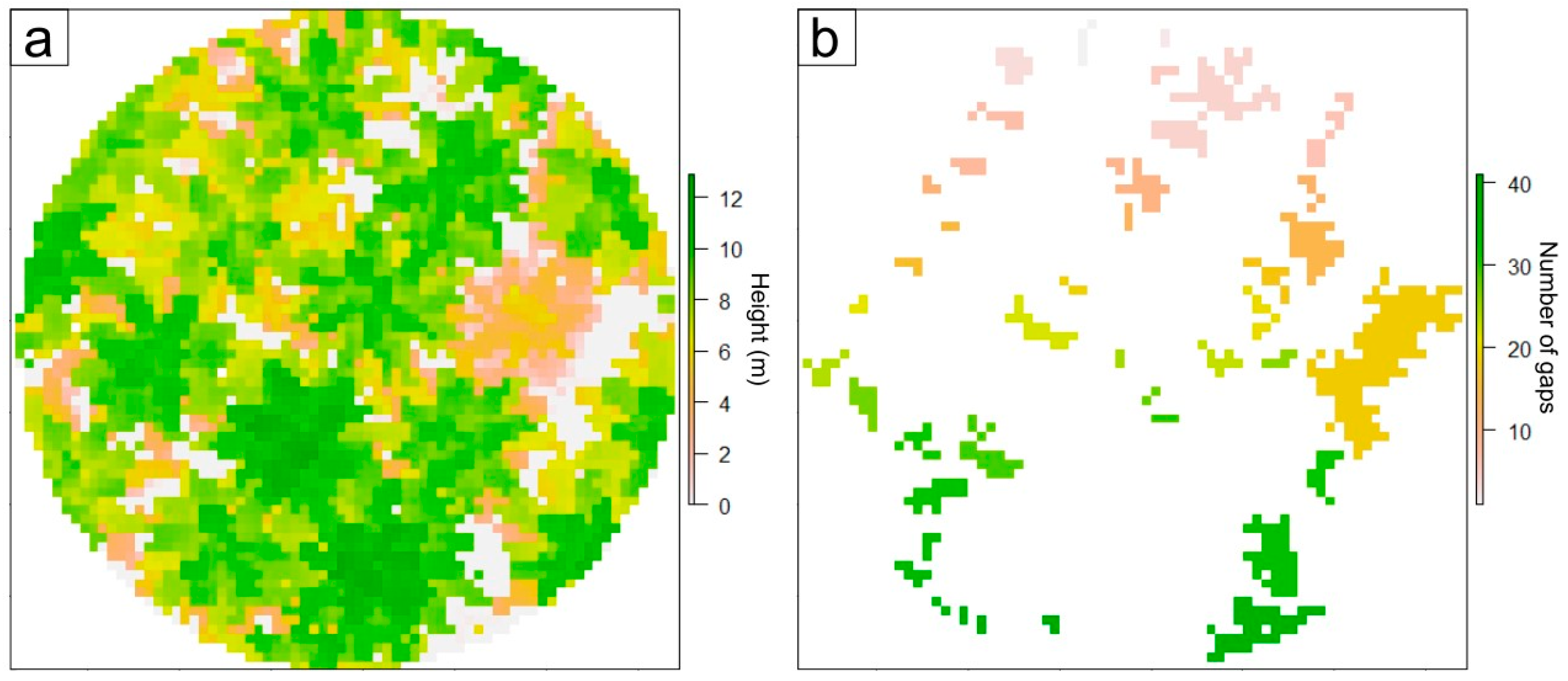
veg_cover (%)Vegetation cover above 2.5 m. Calculated as the inverse of sum_gapArea.
sum_gapAreaTotal extent of gaps > 2.5 m, calculated on a CHM raster with a pixel size of 0.5 m (m2). Obtained using the “GapStats()” function from the ForestGapR package [63]
laiLeaf area index, derived from the vertical distribution of points using the “lai()” function from leafR package [64]
Complexity/Heterogeneity Measures
MetricsDescription
DbBox dimension, a holistic index of vegetation structural complexity. This metric was the only one calculated using the Mathematica software version 12 (Wolfram Research, Champaign, USA) calculated following Seidel [9] and Arseniou et al. [65] but adapted to the lower resolution of ALS point clouds by using a lower cut off of 1 m
zentropyEntropy of height points. Calculated using the “stdmetrics()” function from the lidR package [56]
zkurtKurtosis of height points. Calculated using the “stdmetrics()” function from the lidR package [56]
zskewSkewness of height points. Calculated using the “stdmetrics()” function from the lidR package [56]
zsd (m)Standard deviation of height points. Calculated using the “stdmetrics()” function from the lidR package [56]
rumpleRumple index, a measure of top canopy surface roughness [66]. Calculated using the “rumple_index()” function from lidR [56]
Measures of Vertical Structure
MetricsDescription
pzabove2Number of points above a 2 m height threshold. Calculated using the “stdmetrics()” function from the lidR package [56]
zqNN (m)Percentiles of height returns (NN = 25, 50, 75). Calculated using the “stdmetrics()” function from the lidR package [56]
fhd_shan_eveFoliage Height Diversity, calculated as Shannon evenness, computed using the “FHD” function of the leafR package [64]
fhd_shan_divFoliage Height Diversity, calculated as Shannon diversity, computed using the “FHD” function of the leafR package [64]
enlEffective Number of Layers, a structural complexity index, calculated following Ehbrecht et al. [67]
crCanopy ratio, calculated as (zmax—zq25)/zmax [68]
Measures of Horizontal Structure
MetricsDescription
num_gapsTotal number of gaps in the canopy > 2.5 m, calculated on a CHM raster with a pixel size of 0.5 m. Obtained using the “GapStats()” function from the ForestGapR package [63]
max_gapAreamaximum gap size > 2.5 m, calculated on a CHM raster with a pixel size of 0.5 m (m2). Obtained using the “GapStats()” function from the ForestGapR package [63]
min_gapAreaminimum gap size > 2.5 m, calculated on a CHM raster with a pixel size of 0.5 m (m2). Obtained using the “GapStats()” function from the ForestGapR package [63]
mean_gapAreamean gap size > 2.5 m, calculated on a CHM raster with a pixel size of 0.5 m (m2). Obtained using the “GapStats()” function from the ForestGapR package [63]
Table 2. Information relative to the eigenvalue and significance (p-value) of the different metrics extracted from LiDAR and the four main PCs (i.e., principal components) derived from the PCA analysis. (ns p > 0.05; * p < 0.05; ** p < 0.01; *** p < 0.001).
PC 1PC 2
MetricEigenvaluep-ValueMetricEigenvaluep-Value
pzabove20.97***zq250.57***
veg_cover0.92***mean_gapArea0.51***
zentropy0.92***zkurt0.50***
fhd_shan_div0.91***min_gapArea0.48***
Lai0.89***zq500.36***
fhd_shan_eve0.89***max_gapArea0.36***
zq750.89***zmax0.35***
zq500.87***fhd_shan_div0.31***
Enl0.82***enl0.31***
Db0.82***lai0.30***
Zsd0.79***zq750.29***
Zmax0.76***sum_gapArea0.26***
zq250.73***zskew0.23**
rumple0.59***fhd_shan_eve0.21**
min_gapArea−0.58***zsd0.20**
Zkurt−0.64***veg_cover−0.26***
Cr−0.67***zentropy−0.27***
mean_gapArea−0.76***rumple−0.28***
Zskew−0.81***Db−0.33***
max_gapArea−0.89***cr−0.48***
sum_gapArea−0.92***num_gaps−0.80***
PC 3PC 4
MetricEigenvaluep-valueMetricEigenvaluep-value
rumple0.67***min_gapArea0.62***
Zsd0.52***mean_gapArea0.35***
Cr0.47***num_gaps0.24***
Zmax0.46***zskew−0.18*
Enl0.36***
num_gaps0.34***
Zskew0.33***
zq750.26***
Db−0.18*
fhd_shan_eve−0.19**
zq25−0.22**
Table 3. Confusion matrix for the random forest classification of the 5LU model. OA = overall accuracy; PA = producer’s accuracy; UA = user’s accuracy; Kappa = Cohen’s Kappa.
Predicted
ObservedForestJungle RubberRubberOil PalmTransitional LandPA (%)
Forest4310044.4
Jungle rubber4410044.4
Rubber0042344.4
Oil palm0013533.3
Transitional land0001888.9
UA (%)50.057.157.150.047.1
OA (%)51.1 Kappa0.39
Table 4. Confusion matrix for the random forest classification of the 4LU model. OA = overall accuracy; PA = producer’s accuracy; UA = user’s accuracy; Kappa = Cohen’s Kappa.
Predicted
ObservedForestRubberOil PalmTransitional LandPA (%)
Forest9000100.0
Rubber042344.4
Oil palm017177.8
Transitional land003666.7
UA (%)100.080.080.060.0
OA (%)72.2Kappa0.63
Table 5. List of predictor variables (LiDAR-derived metrics) and relative mean decrease in accuracy (MDA) for each of the five land uses from the 5LU model, shown by decreasing order of importance.
ForestJungle RubberRubberOil PalmTransitional Land
MetricsMDAMetricsMDAMetricsMDAMetricsMDAMetricsMDA
zmax2.1fhd_shan_div1.6zq501.5fhd_shan_div1.9rumple1.9
zq751.7Enl1.4fhd_shan_div1.2lai1.7zsd1.9
zsd1.6zmax1.1zskew1.1zsd1.6zq751.7
zentropy1.5pzabove20.9veg_cover1.0zmax1.5zq501.7
enl1.5fhd_shan_eve0.9zsd0.9zq751.5zskew1.2
fhd_shan_div1.3zentropy0.8pzabove20.8enl1.4zkurt1.1
fhd_shan_eve1.2Lai0.8cr0.7zkurt1.1zmax0.9
zq501.1zkurt0.7sum_gapArea0.7zq250.9veg_cover0.8
zq250.8zq750.7zmax0.6zentropy0.9max_gapArea0.8
cr0.8num_gaps0.5zq750.6fhd_shan_eve0.9enl0.6
zkurt0.7zq500.5zentropy0.5num_gaps0.8pzabove20.6
rumple0.5zq250.4rumple0.3cr0.8zentropy0.5
lai0.4rumple0.4lai0.3zskew0.8mean_gapArea0.3
pzabove20.4Zsd0.2mean_gapArea0.2zq500.7zq250.1
num_gaps0.1Cr0.2zkurt0.1rumple0.5sum_gapArea0.1
zskew0.1max_gapArea0.1zq250.1max_gapArea0.5fhd_shan_eve−0.1
max_gapArea0.0mean_gapArea0.1max_gapArea−0.1pzabove20.3cr−0.2
mean_gapArea−0.1veg_cover0.0enl−0.1mean_gapArea0.0lai−0.3
veg_cover−0.1sum_gapArea−0.2fhd_shan_eve−0.2veg_cover−0.1fhd_shan_div−0.4
sum_gapArea−0.2zskew−0.3num_gaps−0.2sum_gapArea−0.5num_gaps−0.7
Table 6. List of predictor variables (LiDAR-derived metrics) and relative mean decrease in accuracy (MDA) for each of the four land uses from the 4LU model, shown by decreasing order of importance.
ForestRubberOil PalmTransitional Land
MetricsMDAMetricsMDAMetricsMDAMetricsMDA
enl2.2enl1.5fhd_shan_eve1.4zq751.7
zsd1.9zq501.4zsd1.4rumple1.6
lai1.6zskew1.4zq751.3zsd1.5
zmax1.6zmax1.3enl1.3zq501.5
zentropy1.5zsd1.2zq251.2zkurt1.3
fhd_shan_div1.4veg_cover1.1lai1.2enl1.0
zq751.3cr1.1zmax1.1max_gapArea1.0
zq501.0lai0.9rumple0.9min_gapArea0.8
rumple1.0zkurt0.8zkurt0.7zmax0.8
fhd_shan_eve0.9fhd_shan_div0.8num_gaps0.7mean_gapArea0.7
zq250.9Db0.7cr0.7zskew0.7
Db0.9zq750.6zskew0.6pzabove20.6
pzabove20.8zq250.5fhd_shan_div0.6veg_cover0.4
mean_gapArea0.7sum_gapArea0.5pzabove20.6fhd_shan_div0.4
veg_cover0.6rumple0.4Db0.5sum_gapArea0.3
num_gaps0.4fhd_shan_eve0.4zq500.5zentropy0.2
zkurt0.3num_gaps0.3zentropy0.1fhd_shan_eve0.1
cr0.2mean_gapArea0.2sum_gapArea0.1Db0.0
min_gapArea0.0min_gapArea0.0veg_cover0.0num_gaps−0.1
zskew−0.2max_gapArea−0.3mean_gapArea−0.3lai−0.3
max_gapArea−0.4pzabove2−0.4min_gapArea−0.3zq25−0.5
sum_gapArea−0.9zentropy−0.4max_gapArea−0.4cr−0.6
Publisher’s Note: MDPI stays neutral with regard to jurisdictional claims in published maps and institutional affiliations.

