Shared Blocks-Based Ensemble Deep Learning for Shallow Landslide Susceptibility Mapping

Abstract

Natural disaster impact assessment is of the utmost significance for post-disaster recovery, environmental protection, and hazard mitigation plans. With their recent usage in landslide susceptibility mapping, deep learning (DL) architectures have proven their efficiency in many scientific studies. However, some restrictions, including insufficient model variance and limited generalization capabilities, have been reported in the literature. To overcome these restrictions, ensembling DL models has often been preferred as a practical solution. In this study, an ensemble DL architecture, based on shared blocks, was proposed to improve the prediction capability of individual DL models. For this purpose, three DL models, namely Convolutional Neural Network (CNN), Recurrent Neural Network (RNN), and Long Short-Term Memory (LSTM), together with their ensemble form (CNN–RNN–LSTM) were utilized to model landslide susceptibility in Trabzon province, Turkey. The proposed DL architecture produced the highest modeling performance of 0.93, followed by CNN (0.92), RNN (0.91), and LSTM (0.86). Findings proved that the proposed model excelled the performance of the DL models by up to 7% in terms of overall accuracy, which was also confirmed by the Wilcoxon signed-rank test. The area under curve analysis also showed a significant improvement (~4%) in susceptibility map accuracy by the proposed strategy.

1. Introduction

Natural disasters may be described as the occurrence of an extremely hazardous event that has impacts on communities causing damage, disruption, and casualties, leaving the affected communities unable to function normally [1]. Among natural hazards, landslides compose at least 17% of all mortalities caused by natural disasters all over the world, based on the statistics provided by the Center for Research on the Epidemiology of Disasters (CRED) [2]. Landslides, which are characterized by the downslope motions of soil or rock materials under the effect of gravity, have long been affecting human society, natural habitats, and biota in various forms [3,4]. According to the statistics, between 1995 and 2014 more than 3876 landslide activities occurred globally, incurring 163,658 fatalities and 11,689 injuries [5]. In other spatiotemporal-based research, it was reported that non-seismic landslides cost the lives of approximately 56,000 people between 2004 and 2016 [6]. Furthermore, landslides are predominantly responsible for forest and soil denudation, since they modify the topography of the Earth’s surface through the sudden deformations they create. In addition, based on the statistics from the Emergency Events Database [7], landslides cost an estimated 10.8 billion US dollars in economic damage from the 18th to the 20th century, implying the urgent necessity for ongoing assessment and enhancement of efforts to effectively manage and minimize landslide hazards.

The unexpected and harsh implications of landslides have mobilized the global scientific community to take necessary precautions. In this context, the production of landslide susceptibility maps (LSMs) with accurate, up-to-date, and reliable information is prominent in the current literature. With LSMs, the geospatial distribution of landslide and non-landslide zones of the study area under consideration can be characterized. In addition, such maps not only assist extensive solutions to decision makers and public institutions in terms of preparing emergency action plans during the pre-disaster phase, but also serve as a functional tool in land management practices. Moreover, LSMs can be used as a base map in many infrastructure and superstructure investments.

Owing to the complex nature and inconsistent mechanism of landslides, understanding the major triggering factors underlying their occurrences and modeling their spatial probability have been challenging tasks, mainly researched through statistical, deterministic, and heuristic approaches [8,9]. The statistical methods are usually constructed using linear correction analysis between historical landslides and predisposing factors. On the other hand, deterministic methods require the estimations of quantitative measures of stability factors across given a region and several necessary parameters (e.g., soil strength and layer thickness) [10]. In heuristic approaches, expert opinions are employed for predicting landslide hazards by using predisposing factors, substantially involving the expert knowledge system and analytical hierarchy process. A given hazard is rated considering the professional judgment of the analyst conducting the investigation. The major challenge of heuristic approaches is the inadequacy of information related to the study region, which occasionally results in undesirable generalizations [11]. Although these techniques are intensively utilized for the generation of LSMs, they have major limitations of requiring expert opinion and being applicable in only homogenous geomorphic settings [12,13]. Therefore, most efforts have been devoted to solving the problem by using more robust models. In parallel with the rapid improvements in artificial intelligence and computer science, a new methodological concept called machine learning (ML) has become apparent in many domains. These developments have also opened new horizons in landslide susceptibility mapping studies. More specifically, the transition from conventional knowledge-driven methods to data-driven strategies inherently had a direct impact on the predictive performances of LSMs, and researchers emphasized that the new strategy was more robust than previous approaches [14,15,16]. Until the present, numerous ML approaches in a broad spectrum have been actively pursued. Some of these are based on decision trees, which have a structure used to divide into smaller clusters by applying a set of decision rules (i.e., decision tree and random forest) [17,18]. Some of them (i.e., support vector machines) are founded on the vector space-based approaches that try to seek a decision boundary between classes [19]. Others are based on gradient boosting methodology (i.e., gradient boosting machine, CatBoost, and XGBoost), employing the principle of repetitively using patterns in residuals and strengthening and improving a model with poor predictions [20,21,22].

Within the past few years, a new and evolving paradigm, namely deep learning (DL), has been introduced to overcome some of the inherent restrictions of ML models and boost the predictive quality of a produced model. DL algorithms do not need prior information, since they can efficiently find relevant information across disparate datasets and get the best parameters for creating models during the model training process. Moreover, the impact of overfitting on the prediction accuracy of the DL model can be eliminated. Due to the above-mentioned distinctive features, DL models have been intensively utilized in natural disaster impact assessment—such as flooding [23], wildfires [24], and tsunamis [25]—to understand the complex and dynamic structures of such phenomena. Previous studies showed that DL algorithms, including Convolutional Neural Networks (CNNs), Recurrent Neural Networks (RNNs), and Long Short-Term Memories (LSTMs), have produced remarkable predictive performances in the estimation of landslide vulnerability [26,27,28,29,30]. For instance, [31] investigated landslide susceptibility prediction using support vector machine (SVM), 1D-CNN, and artificial neural networks (ANN) in the Yangyang province, South Korea, and reported that CNN was superior to the ANN and SVM due to its ability to deal with geospatial correlations via convolution and pooling functionalities. Likewise, RNN was used to tackle the same problem and was found to have an effective predictive ability for landslide susceptibility mapping [32,33]. Research in [34] also applied RNN and its variants to produce an LSM of Yongxin County, China, and proved their effectiveness. Likewise, [29] employed three inductive learning algorithms, namely decision tree, SVM, and backpropagation neural network, together with LSTM, to forecast spatial probabilities of landslide risk in the China–Nepal Highway. Results indicated that LSTM outperformed the other ML algorithms because of its ability to understand the time sequence with extended temporal constraints.

Despite the recent prevalent use of single DL algorithms in landslide susceptibility mapping studies, some drawbacks, namely insufficient model variance, less model generalization, and limited model performance have been reported [28]. Each DL architecture has its a specialized structure for specific applications. In such circumstances, ensembling several DL models can boost the accuracy of the output, thereby allowing the main model to be generalized, also providing an improved nonlinear representation [34]. Although the ensemble scheme has been widely employed for traditional ML techniques [35,36], the use of this concept for DL models is still an inactive topic in the generation of LSM practices. Therefore, in this study, shared layers architecture, constructing an ensemble framework through individual DL algorithms, was adopted. Shared layers are an important strategy for generalizing DL models, ensuring the process of merging layers of numerous trained DL models into a new model. The shared layers are regarded as a feasible and effective method for minimizing the number of parameters in DL models. Previous research has shown that the overall prediction quality in the ensemble DL model may be improved by processing the tasks cooperatively and transferring information between the models [37].

In the present work, three popular individual DL algorithms (i.e., CNN, RNN, and LSTM) and an ensemble DL model (RNN–CNN–LSTM), based on the shared layers blocks, are employed for generating LSMs of the Trabzon province, located in the northeast part of Turkey. The ultimate motivation of the study is to show the ease of use and effectiveness of the ensemble DL architecture, together with its superiority over the individual DL methods in the landslide susceptibility prediction. The additional objective of the work is to provide an explainable decision-making mechanism of the proposed DL structure with the SHapley Additive exPlanations (SHAP) approach. The novelty of this work lies in the implementation of the ensemble DL strategy concept by employing the shared layers architecture in landslide susceptibility mapping to compensate for the above-mentioned restrictions of individual DL algorithms. To this end, the importance scores of each landslide conditioning factor were initially estimated utilizing the correlation-based feature selection (CFS) technique. Thus, potential collinearity in the dataset was sought to feed the DL architecture with more suitable features. The predictive performances of the produced LSMs were evaluated using six well-known accuracy metrics, namely overall accuracy (OA), precision, recall, F1-score, Kappa coefficient, and area under the receiver operating curve (AUC). Moreover, a statistical significance test (i.e., Wilcoxon signed-rank test) was implemented to make a sound comparison of the predictive performances of the DL models. Finally, the contribution of each predisposing factor on the proposed ensemble DL architecture is explained using the SHAP method, based on game theory.

2. Study Area and Dataset

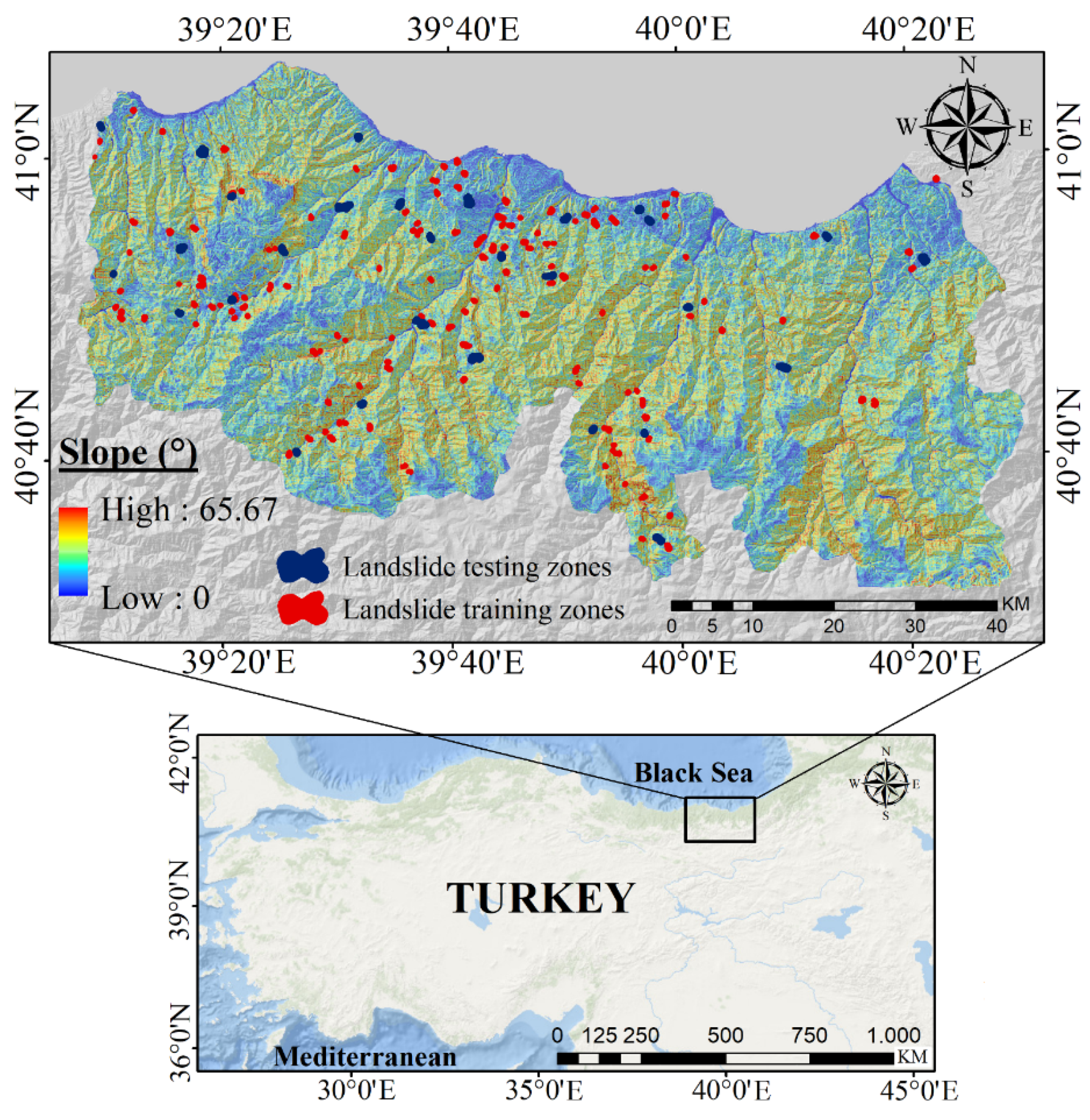
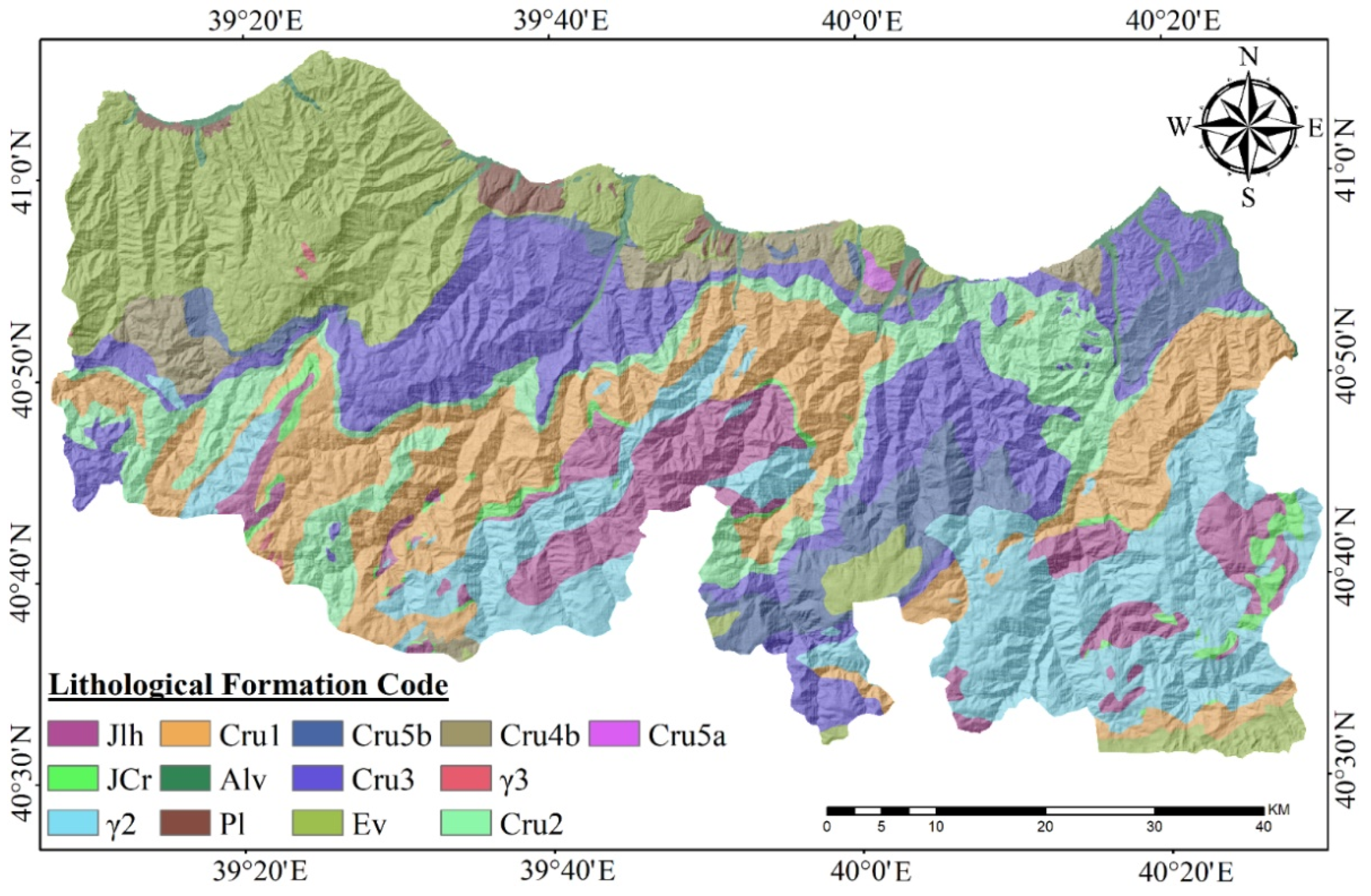
2.1. Description of the Study Area

Trabzon province, which is situated in the Eastern Black Sea coast of Turkey, was considered as the area of interest since it is one of the regions intensely exposed to landslide phenomena. The study area is geographically located 41°08′ and 40°30′ latitudes and 39°15′ and 40°15′ longitudes, which occupies a land of approximately 4664 km² (Figure 1). It is a narrow flat land nearby the sea and is characterized by rough and hilly topography extending vertically to the seashore.

Topographically, the study area has elevations ranging from 0 to 3354 m and slope angles up to 70°. Morphologic, climatic, and physiographic characteristics of the region facilitate occurrences of landslide activities. In the region dominated by the characteristics of the Black Sea climate, the annual mean precipitations and temperature are 819 mm and 14.7 °C, respectively. Nonetheless, the precipitation pattern is erratic, with some seasons of sparse rain followed by prolonged torrential rains. Such excessive rainfall accelerates the rate of weathering, significantly weakening the resilience of the covering materials to the potential of mass movement [38]. In the Eastern Black Sea region, particularly in the Trabzon province, landslide activities are a long-term and escalating challenge for the local community. As a matter of fact, in 1929, 1950, 1952, 1985, 1988, and 1990, a great deal of life was lost in this region and there have been huge landslides causing property loss [39]. For instance, 65 people lost their lives in the Maçka/Çatak region and the area suffered substantial financial losses due to the heavy rain [39]. Besides, more than 150 landslides occurred between 2005 and 2008 in places with excessive precipitation and escarpments; as a result, many residential buildings were damaged, and 460 buildings became uninhabitable [40].

Geological structures of the region under consideration are primarily characterized by Pliocene (Pl), Eocene (γ₂, γ₃, Ev), Upper Cretaceous-Paleocene (Cru1, Cru2, Cru3, Cru4b, Cru5b, Cru5a), Upper Jurassic-Lower Cretaceous (JCr), and Secondary and Tertiary eras composing Lias-Dogger (Jlh) (Figure 2). Some units are predominantly derived from magmatic rocks, such as granitic, basaltic, and dacitic rocks, while certain units incorporate sedimentary units such as sand–mud stone, limestone, alluvial deposits. In the region, shallow landslide incidence has continually risen as a result of the highly saturated loamy formations [41]. Apart from the triggering factors of landslide occurrences, human intervention (i.e., anthropogenic factors), including infrastructural construction, skewed urbanization, and deforestation have also severe impacts on the initiation of mass movement activities.

2.2. Landslide Inventory Map

Evaluation of landslide susceptibility is generally evaluated based on the fundamental hypothesis that further landslide activities will presumably happen under similar circumstances as previous landslides [8]. Additionally, historical mass movements’ locations provide insight and assist comprehensible inferences for links between spatial distributions of future landslides and factors contributing to these phenomena. Therefore, landslide inventory is considered as one of the most key tools in predicting further events [14].

In the present work, landslide samples were digitized as polygons from a topographic base map with 1/25,000 scale to produce landslide inventory procured by the General Directorate of Mineral Research and Exploration of Turkey. It should be noted that all recorded historical landslides have shallow translational characteristics, owing to the prolonged precipitation in the study area. Another important step in the landslide susceptibility mapping procedure is the determination of the sampling strategy to be used in the extraction of landslide instances, which directly affects the predictive performances of the produced LSMs. Therefore, this issue has always been under constant investigation and is a well-documented problem within the current literature [42,43]. Several strategies, such as centroids [44] and seed cells [45] have been employed to deal with the representation of the landslide polygons before the model training phase. In this current work, one of the well-known sampling methods—the polygons of landslides for representing geospatial position, utilized by several researchers [46,47,48]—was adopted as a landslide sampling strategy. The main scarp of each landslide sample extracted from the accumulation/depletion zone was later considered as a vector polygon. The existing 168 landslide polygons on the inventory map were transformed into a raster version. The overall area exposed by landslide phenomena is approximately 15 km² while the smallest and largest landslide areas were 136 m² and 496,108 m², respectively. It should be emphasized that every pixel or landslide sample corresponds to a 30 × 30 m grid on the ground. On the other hand, proper representation of non-landslide zones is one of the highest priority steps for constructing landslide inventory. In case of the absence of ground truth data for non-landslide samples, the methodology suggested by [10] is suitable and easy to implement. This approach depends on two main facts: that a landslide event is not probable to occur (i) on the surface of stagnant water or river channels, or (ii) on topographies with slope angles not exceeding 5 degrees. Subsequently, the stratified random sampling approach is adopted to create non-landslide and landslide samples. Finally, it is worth mentioning that a total of 16,718 landslide instances (i.e., pixels) were extracted and an equal number of non-landslide instances were collected in order to avoid potential biases and inferences stemming from the unbalanced dataset, and to make a sound comparison for the produced DL models through accuracy assessment metrics.

2.3. Landslide Predisposing Factors

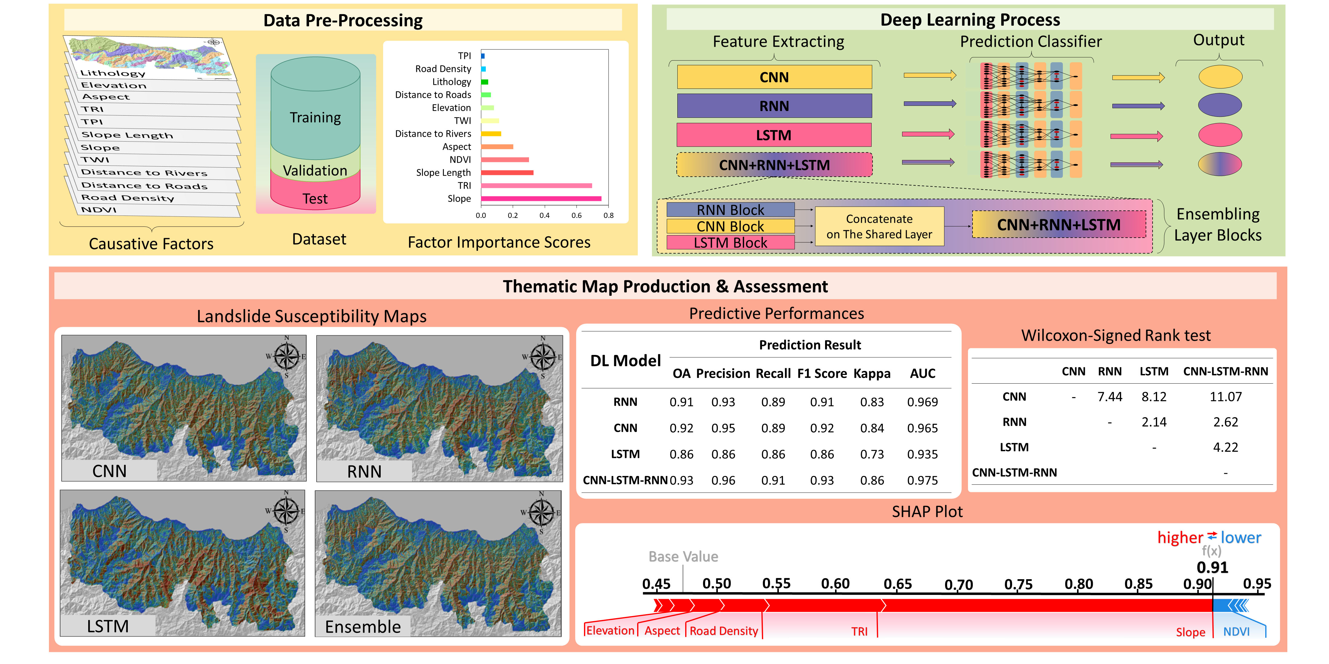
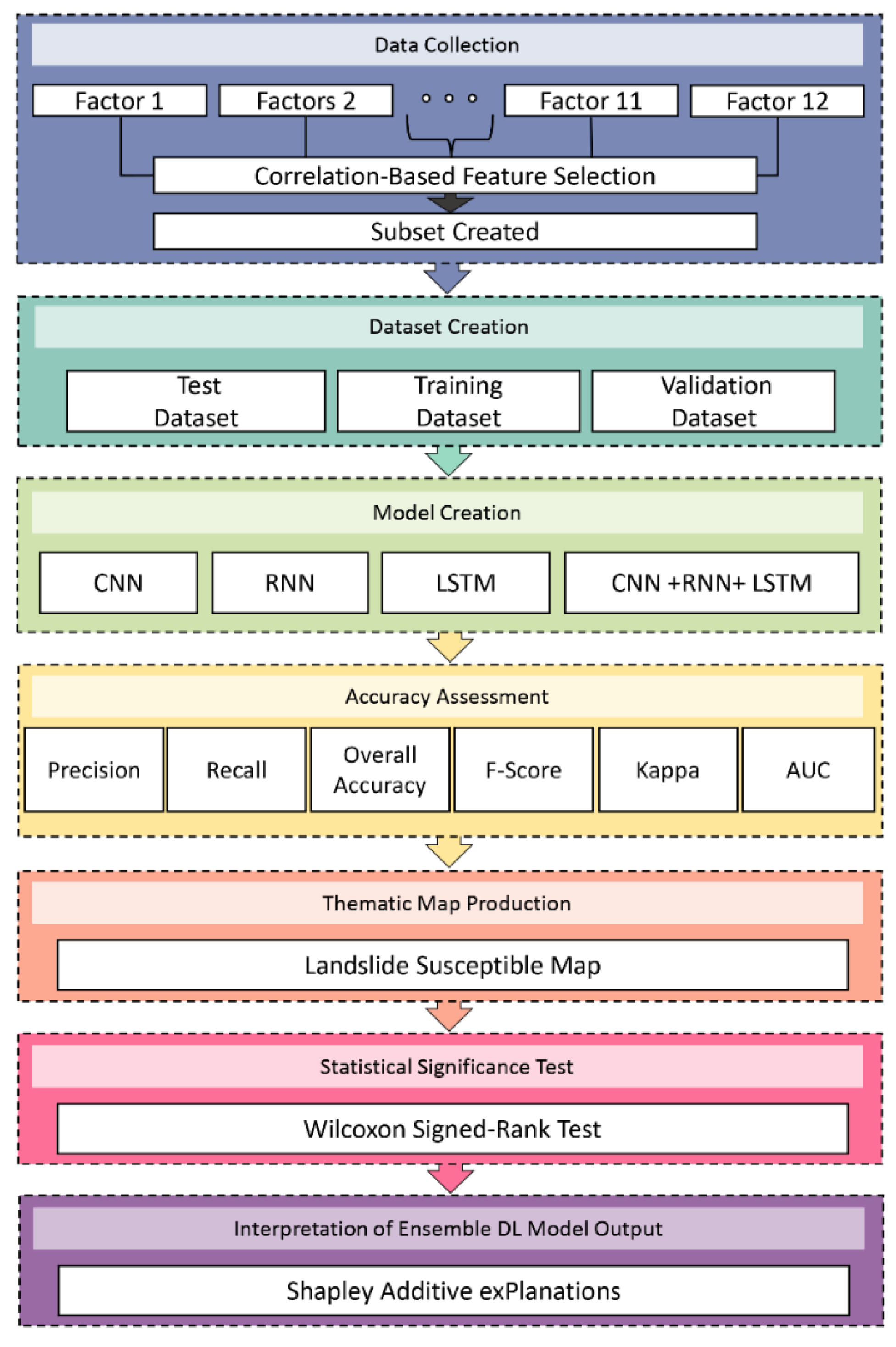
The correct identification of contributing factors plays a significant role in the robustness and reliability of produced resultant LSMs, since they have an important implication on the performances of the ML models. Meanwhile, such factors are also expected to be consistent with the general feature of the study area. In the current work, as major geomorphological, hydrological, geological, and environmental features of the study area, a total of 12 predisposing factors—including lithology, elevation, aspect, topographic wetness index (TWI), topographic roughness index (TRI), topographic position index (TPI), slope length, slope, distance to roads, road density, distance to rivers, and normalized difference vegetation index (NDVI)—were considered, based on both of the previous research studies conducted in the same region [48,49] (

Table 1. Data source and scale/resolution information of landslide predisposing factors.

Major Factors	Sub-Factors	Source	Scale/Resolution
Geology	Lithology	General Directorate of Mineral Research and Exploration of Turkey (http://www.mta.gov.tr (accessed on 4 October 2021))	1:100,000
Topographical	Elevation (m)—DEM	Shuttle Radar Topography Mission (SRTM- https://earthexplorer.usgs.gov/ (accessed on 4 October 2021))	30 m
	Aspect	DEM
	TRI
	TPI
	Slope Length
	Slope (°)
Hydrological	TWI	DEM	30 m
	Distance to Rivers	Digitized existing river networks
Environmental	Distance to Roads	Digitized existing road and river networks	30 m
	Road Density
	NDVI	Landsat-8 Operational Land Imager (OLI) multispectral image (2016), (https://earthexplorer.usgs.gov/(accessed on 4 October 2021))

).

The digital elevation model (DEM), which is the main source for generating causative factors, was provided by Shuttle Radar Topography Mission (SRTM). Seven thematic maps (i.e., factors) including elevation, aspect, TWI, TRI, TPI, slope length, and slope were produced from DEM. Distance to roads and distance to rivers were produced with the Euclidean distance function, and road density was produced using existing road network data. NDVI, which provides information about the health and density of green vegetation, was produced by using the Red and NIR bands of Landsat-8 OLI. The lithology map of the region, composing 13 units, was supplied by the General Directorate of Mineral Research and Exploration, Turkey.

3. Methodology

In the literature, a wide range of methodological frameworks have been adopted to generate LSMs. In this paper, the process of LSM production comprises five key points. The first stage involves acquiring landslide contributing factors, developing a landslide inventory geospatial database, and measuring the contribution to modeling performance of each factor through the correlation-based feature selection. The prepared dataset was later divided into training (80%) (for model training) and test (20%) (for performance evaluation of the produced models) parts. Afterward, the training data were split into two sections, namely training (80%) and validation (20%) for checking whether the models are overfitting. In the third stage, both single and ensemble DL shared layers architecture models were established to build the descriptive structure. Later, six well-known accuracy assessment criteria and a statistical significance test were considered to assess and compare the predictive accuracies of produced DL models. The last stage comprises the generating of LSMs of the study area under consideration. Figure 3 depicts the described methodology adopted in the study. The causative factors were fed into the CNN, RNN, and LSTM models, which were developed in Python using Jupyter Notebook using Keras, Pandas, and Sklearn libraries.

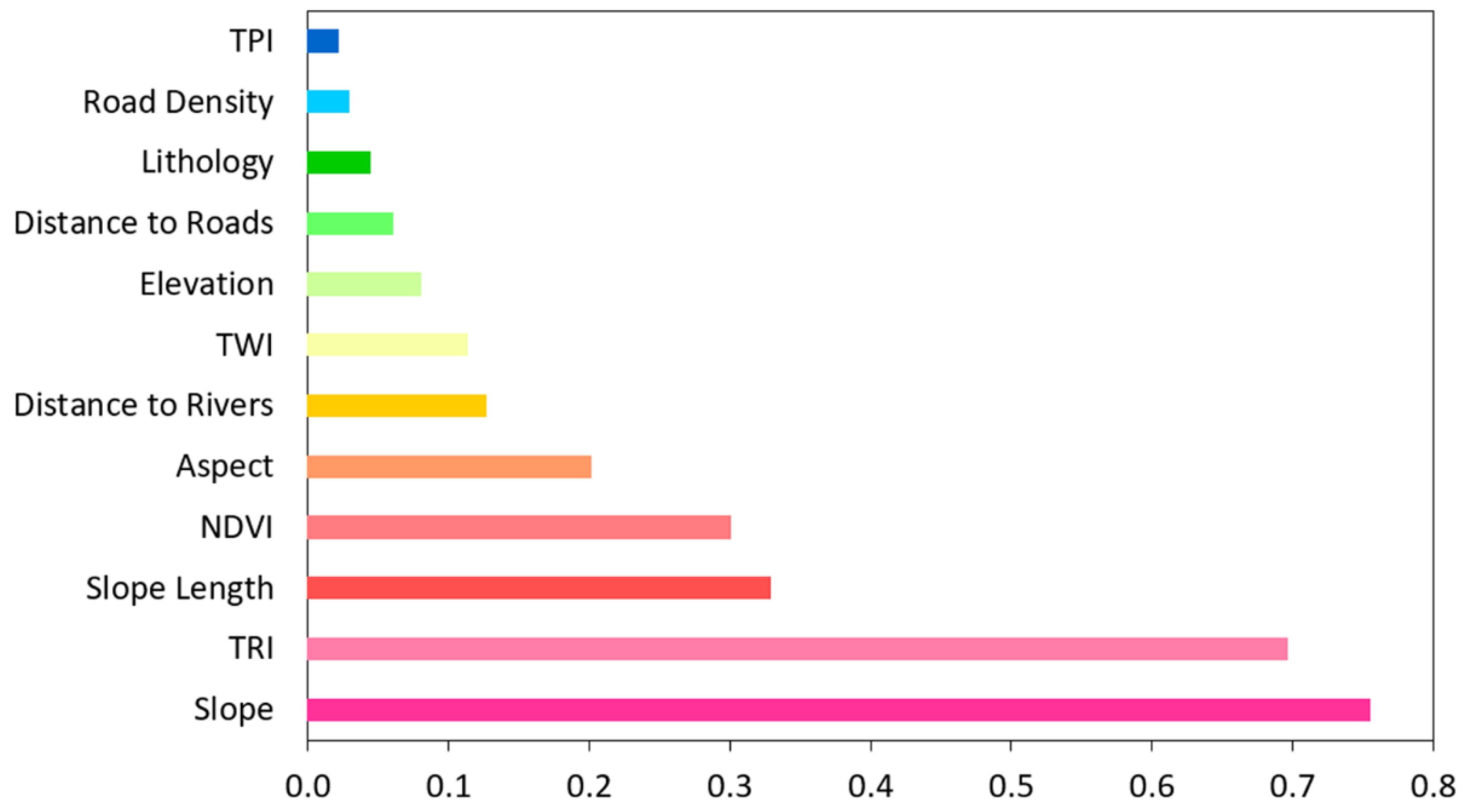
3.1. Correlation-Based Feature Selection

Choosing the most significant landslide causative factors is a fundamental point before the stage of modeling an ML algorithm. In this context, feature selection (FS) techniques not only boost the performances of the models but also improve the generalization capacity and model interpretability. Since the FS process generally reduces the dimension of input variables and storage requirements by eliminating unnecessary information, it decreases computational cost and multicollinearity between the variables. Because of the distinct advantages of the FS methods, they have been recently used in the generation of LSM studies for the selection of most contributing factors [50,51].

In the study, a correlation-based feature selection (CFS) technique was implemented to quantify the mean merit of each contributing factor. The factors with greater correlation coefficient scores have more contribution to the model while zero correlation coefficient implies no contribution, and thus could be discarded from the dataset. The CFS method assesses the correlation of subsets of the entire landslide conditioning factor space by considering the following merit function:

$$r_c=\frac{k\overline{r_{cf}}}{\sqrt{k+k\left(k-1\right)\overline{c_{ff}}}}$$

(1)

where $r_c$ implies the total correlation among factors and the classes of the dependent variable (e.g., landslide and non-landslide); k represents the number of predisposing factors; $\overline{r_{cf}}$ indicates the mean correlation value of the target variable and factors; and $c_{ff}$ denotes the mean factor class correlation.

3.2. Deep Learning Methods

The research of artificial neural networks (NNs) has evolved into the paradigm of DL. DL models are represented by several layers, including batch normalization (BN), flatten, dense, and dropout. The layer of BN is used to establish a consistent distribution of data during training [52]. Furthermore, the flattening layer is used to compress two- or three-dimensional training data to one dimension [53]. The number of units in the model layers must be limited to minimize model dimensions using dense layer structures. The dropout layer is followed by the after dense layer in the DL model. Concisely, the specific neurons dropped out, operating with a random value in the process of forward-propagation, therefore increasing the generalization of the model [54]. The activation functions have a significant role in DL-based architectures. The derivatives of these functions are multiplied using the backpropagation method, and thus, the selected activation function ought to be differentiable. As a consequence, activation functions should be selected in accordance with the models used in the application of DL [55]. In particular, the sigmoid activation function is commonly employed in landslide susceptibility prediction research because the calculation of landslide vulnerability is fundamentally a nonlinear logistic regression topic. The probability of classification in the DL model can also be calculated using the sigmoid function, which represents the vulnerability of a landslide at a specific location [34,56,57].

3.2.1. Convolutional Neural Network (CNN)

CNN is commonly utilized as a feed forward NN that involves convolution processing, including pooling, normalization, dense, dropout, and output layers. CNN models can acquire the outstanding feature properties of the dataset, allowing it to distinguish without the need for human-driven, complicated rules. CNNs may become in a variety of sizes, but they all have input, hidden, and output layers. The input layer takes a one-dimensional matrix with a feature value for each element of input data in the 1D CNN model. Each convolutional layer is composed of some convolutional filters, and the parameters of each process are tuned using back-propagation algorithms. The dataset is convolved using a series of trainable filters which completely sweep the dataset, generating a series of feature maps. Thereby, the most important features of the dataset are extracted in convolutional processing. Herein, this process can continually lower the data dimensionality, resulting in a decrease in the number of parameters and the cost of computing. Thus, the problem of overfitting can be prevented. The following abbreviated equation represents the basic functions performed by all types of 1D CNN (2):

$$I_j^{l }=f ({\displaystyle \sum }_{i=1}^N{I}_i^{l-1}\ast c_{ij }^l+b_j^l)$$

(2)

where c is the number of convolution filters, j points out the extent of convolutional filters, and N is assigned as the channel input number $I_i^{l-1}$. Moreover, b indicates the bias of filters, f refers to the activation functions, and ($\ast$) exemplifies the operator of convolution [58]. On the other hand, CNN offers distinct benefits in many applications with its unique structure of the shared weights, hierarchical feature, and local connectivity [59,60]. Particularly, the redundant factors in the dataset are eliminated using CNN, obtaining just the meaningful information for the LSM application [61].

3.2.2. Recurrent Neural Network (RNN)

RNN, a prominent DL approach, excels at the tasks of sequence analysis. In contrast with CNN, it can handle sequential data utilizing recurrent states, which may acquire meaningful information from both the current and past stages. This indicates that RNN has a strong capacity to extract critical information from the dataset [28]. Therefore, they are highly strong in computational calculation due to the absence of internal states of the RNN [62]. RNNs have attracted much interest recently for their tackling a variety of difficult issues involving sequential data processing. Because a temporal variability of the sequential signal is closely similar to a factor information variability of pixels, the same concept can be used for the LSM pixel unit. Ultimately, RNN uses a recurrent methodology to describe data correlation and variability, with the parameters of the network established while training with the sampled data [33]. The basic architecture of a conventional RNN is shown in Figure 4.

Theoretically, the formula of the basic RNN’s hidden units could be given as follows:

$$h_t=tan h \left( W_x x_t+W_h h_{t-1}+b\right)$$

(3)

where $x_t$ indicates the input data and $h_t$represents the cell state at duration t in the hidden layer, that is derived using cell state, which is shown as $h_{t-1}$ at duration t−1, and also the input data ($x_t$) at duration t. Furthermore, $W_h$ and $W_x$ are temporally shared coefficients in the cell unit. The output of RNN is relied on by both input data in the current duration and the computations in a hidden state from the previous duration [63]. The RNN model is one of the feasible and useful techniques for improving landslide prediction accuracy [32].

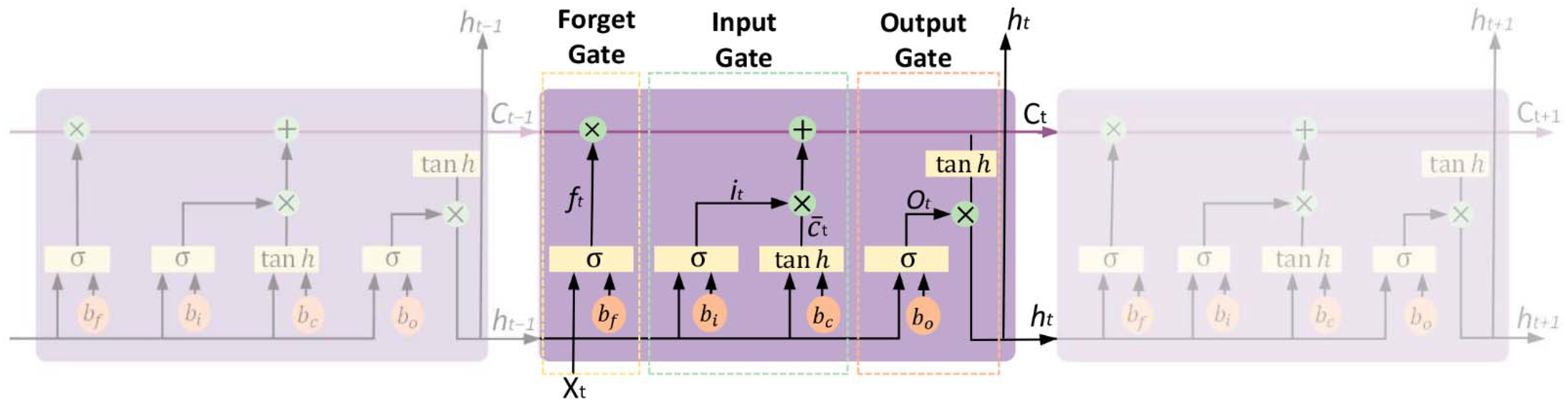
3.2.3. Long Short-Term Memory (LSTM)

A popular technique, LSTM, uses a more advanced recurrent structure to overcome the limitation of the RNN model [64]. The structure of LSTM contains input, one/several hidden, and output layers. When more detailed information is given, a typical LSTM memory block consists of a unit to take information to the unit state, an input gate to manage the amount of unit state update, an output gate to regulate the level of the unit state contributed to output state, and a forget gate to check the level of unit initialized. To calculate the first output and the latest updated unit state, the LSTM layer uses the onset of the state of the network and the input at the initial step [65]. The unit of LSTM is shown in Figure 5.

When the operations of the LSTM unit are implemented to the input dataset with forward propagation, the updating equations for the gate of forget, the gate of input, and the gate of output are as presented in Figure 5 and the equations below.

$$f_t=\sigma \left(W_f·\left[h_{t-1}, x_t\right]+b_f\right)$$

(4)

$$i_t=\sigma \left(W_i·\left[h_{t-1}, x_t\right]+b_i\right)$$

(5)

$$o_t=\sigma \left(W_o·\left[h_{t-1}, x_t\right]+b_o\right)$$

(6)

$${\overline{c}}_t=tanh\left(W_c·\left[h_{t-1}, x_t\right]+b_c\right)$$

(7)

$$c_t=f_t\ast c_{t-1}+i_t\ast {\overline{c}}_t$$

(8)

$$h_t=o_t\ast tan h \left(c_t\right)$$

(9)

where $\sigma$ is represented by the sigmoid function and $c_t$ implies the state of the memory cell at duration $t$. The weight matrices of cell gate and bias from all gates are $W_{f,i,o,c}$ and $b_{f,i,o,c}$, respectively. The unit of LSTM involves a hidden state, with $h_{t-1}$ expressing the hidden state of the previous duration and $h_t$ denoting the hidden state of the current duration. LSTM additionally has the state of the cell, which is described by $c_{t-1}$ for the previous and current durations, respectively. The hidden state is referred to in short-term memory, whereas the cell state is recognized in long-term memory. $h_{t-1} \mathrm{and} x_t$ are analyzed with $c_{t-1}$ at the cell state and the DL, the model determines whether to output 0 (forget entire information) or 1 (store whole information) for each cell. The following stage determines which new data will be held in the unit cell [53]. These systems could be able to generalize the dependencies and are especially appropriate for a sequential dataset, allowing it to be utilized in the generation of LSM.

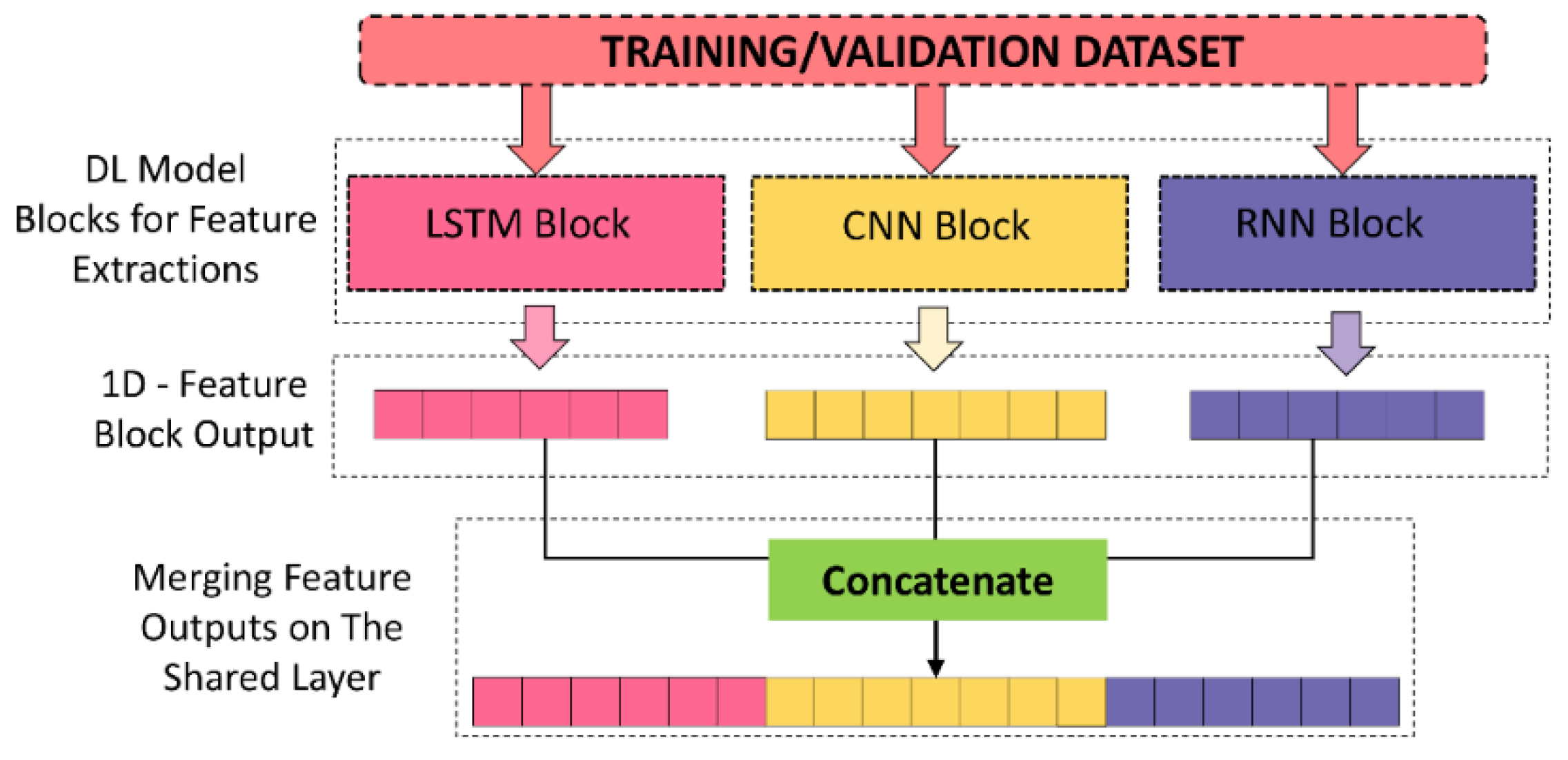
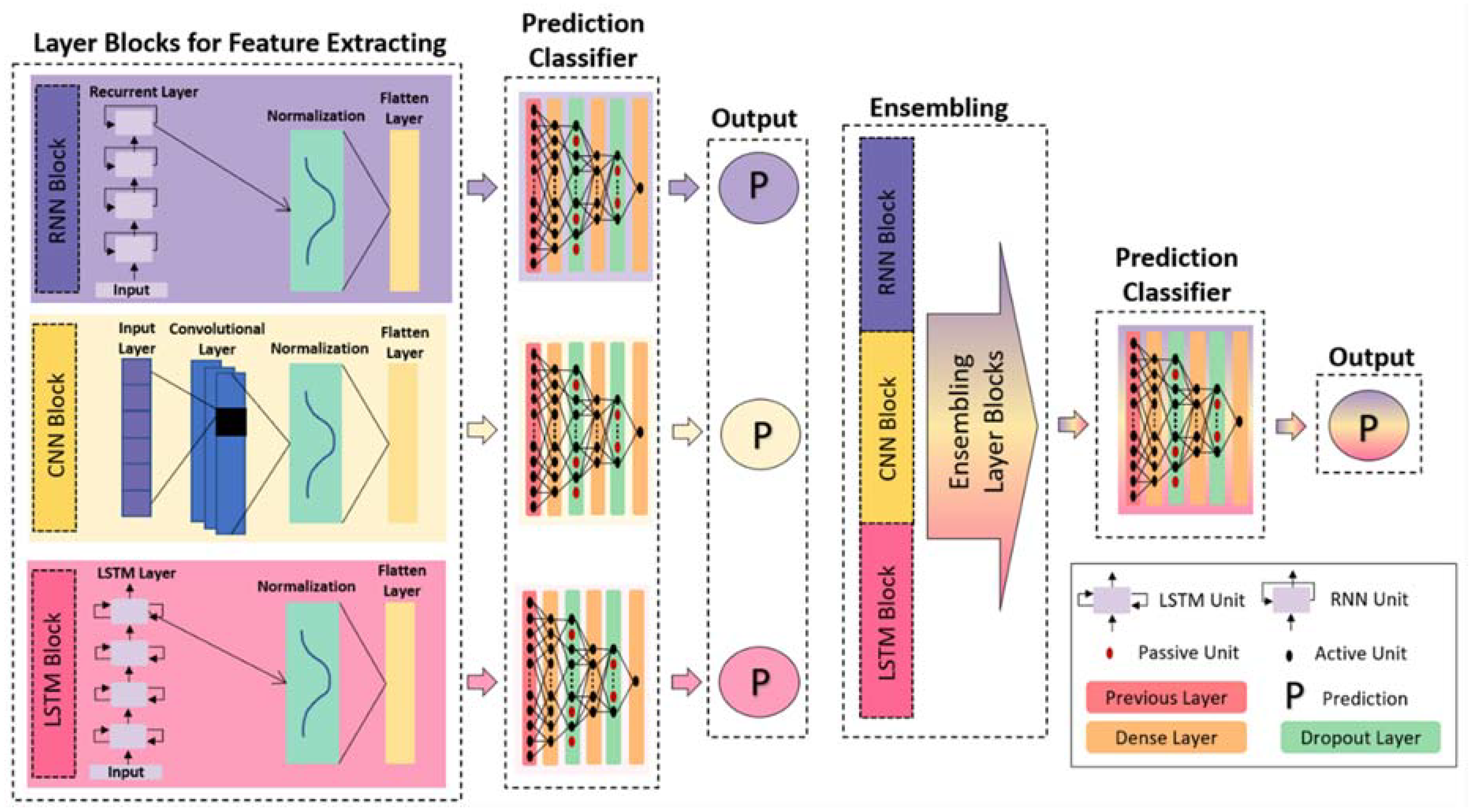
3.2.4. Ensemble DL with Shared Layers Approach

In the production of an LSM, one of the most challenging and critical tasks is the determination of optimal modeling technique which directly affects the produced susceptibility models. In the literature, a large proportion of inductive learning algorithms ranging from conventional statistical-based methods to DL algorithms has been employed for susceptibility mapping [54,66,67,68]. However, the selection of ideal modeling algorithms is still the subject of research, and there are still no globally agreed clear frameworks or guidelines. In the light of this information, rather than choosing a specific learning algorithm, those were combined under an ensemble scheme, based on a shared layers strategy to produce a more stable and robust LSM in the study. On the fundamental basis, the ensemble learning paradigm refers to the combination of several single (i.e., individual) inductive learning algorithms to accomplish better generalization predictive performances [69]. Compared to single DL models, the ensemble DL approach has the advantage of achieving more stable and robust results by aggregating the results of individual DL algorithms [70].

Various networks containing different parameters could be used to acquire the dioristic character of data. Different NNs use the same parameters, which contributes to speeding the process of training and preventing overfitting [71]. In theory, the model layers at every training part are shared with the weights of the similar layers in the other training parts. Moreover, the extracted features from each training part are merged and sent into the concatenated layer (Figure 6). As a result, the high variance within the model is reduced, and also it contributes to the generalization of the model [72]. On the other hand, the number of model parameters rises as the architecture of the model is deeper, even though the previous studies have accomplished noteworthy advancement in training high deeper models.

3.2.5. Description of Network Architectures

In the present study, all networks consist of two main parts. The first part involves the RNN–CNN–LSTM layer blocks for extracting features, and the second part includes dropout and dense layers to calculate the prediction of the classification procedure. These layer blocks contain BN and flattening layers in the DL models. Furthermore, the trial-and-error technique was utilized to seek the best parameters (i.e., epoch number, batch size, the unit number of layer block, activation function, the optimizer, and loss function) to objectively characterize the behaviors of the DL models. The parameters of DL models used in the study are shown in

Table 2. The model parameters of DL architectures.

Model Parameters	CNN	RNN	LSTM
Input dimension	12 × 1	12 × 1	12 × 1
The number of units	16	16	16
Kernel size	2	-	-
Activation function	ReLu, sigmoid, tanh	sigmoid, tanh	sigmoid, tanh
Dense unit	20, 10 and 1	20, 10 and 1	20, 10 and 1
Dropout ratio	0.2	0.2	0.2
Optimizer	Adagrad	Adagrad	Adagrad
Loss function	MSE	MSE	MSE
Maximum epoch	20	20	140
Batch size	32	32	32
Total parameters	3873	913	1777

.

After executing CNN, RNN, and LSTM layers, the data normalization stage was executed by using the BN layer in the layer blocks. The last process in these layer blocks is the flattening stage, since this step is necessary so that they can be concatenated with other layer blocks. Besides, the sigmoid function was selected as an activation function to increase the model nonlinearity; thus, landslide probability with a range between 0 and 1 was quickly computed. Meanwhile, out of 12 landslide predisposing factors, only lithology has a discrete structure, which represents countable data type, while the remaining 11 factors (i.e., topographical, hydrological, and environmental) are in continuous numeric format. Except for single LSTM, the highest number of epochs was set to 20 for all models, because a rapid LSM assessment was required. However, the epoch number was 140 in the single LSTM model for better training. During the implementation phase, the models with only CNN, RNN, and LSTM blocks were trained initially for extracting features. The outputs of these models were acquired using a prediction classifier consisting of dropout and dense layers. In the proposed ensemble DL model, these single DL blocks were ensembled in the same layer; thus, the different features of the data can be captured. In the final stage, the classifier prediction component was inserted into the ensemble DL block, and the final output was generated. For utilizing the concatenate function, four distinct models were created, as shown in Figure 7. The objective of combining all these models was to examine the influence of learning distinguishable characteristics of different DL architectures (i.e., CNN, RNN, and LSTM) on the same dataset.

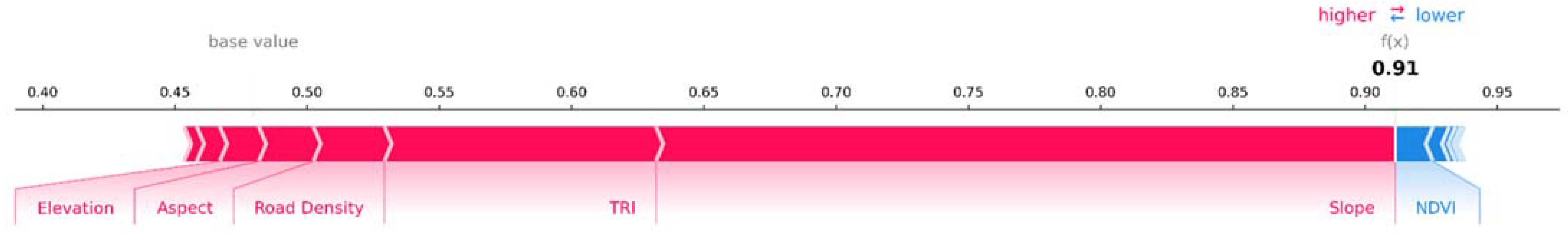
3.2.6. Interpretation of DL Model Output

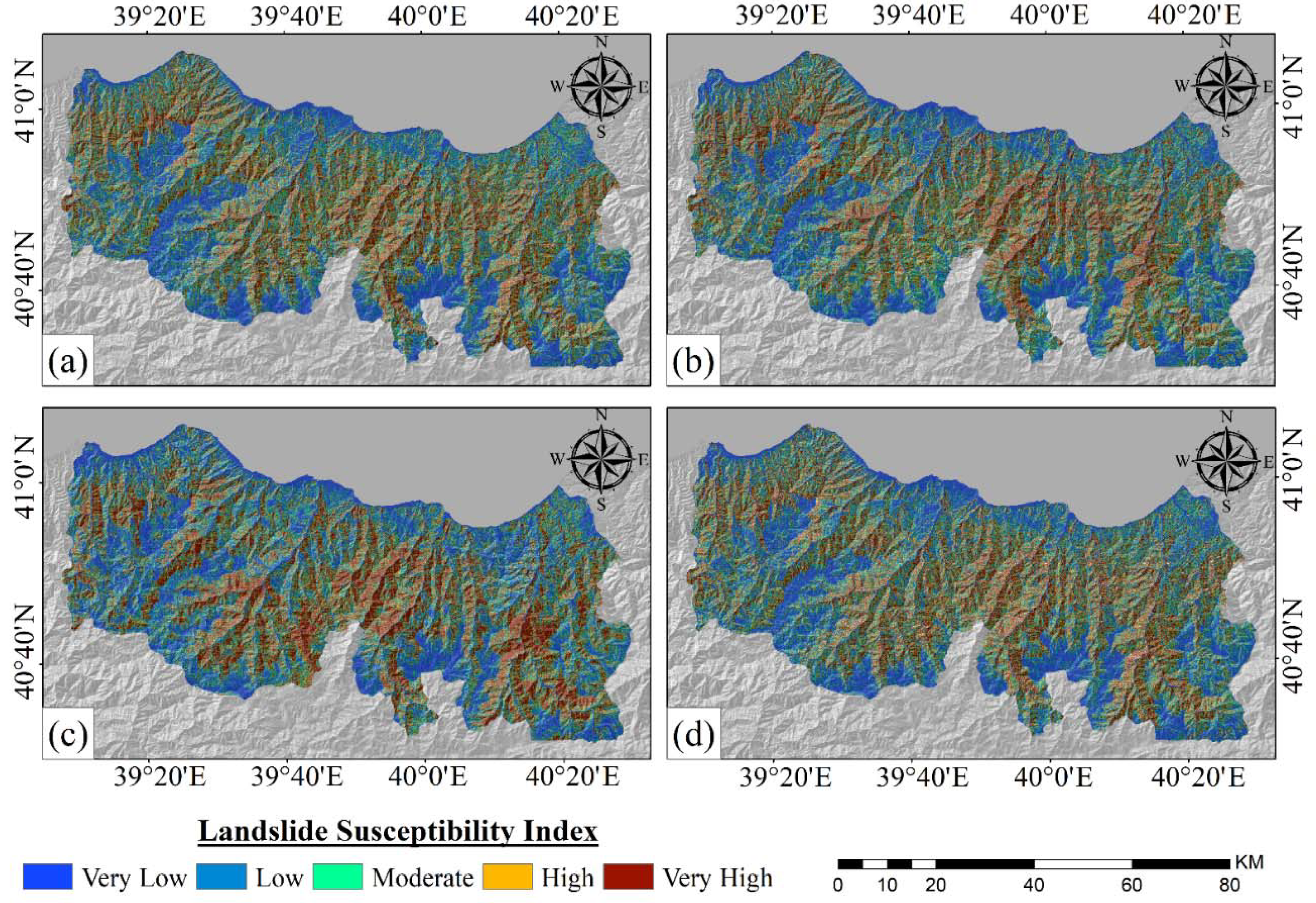
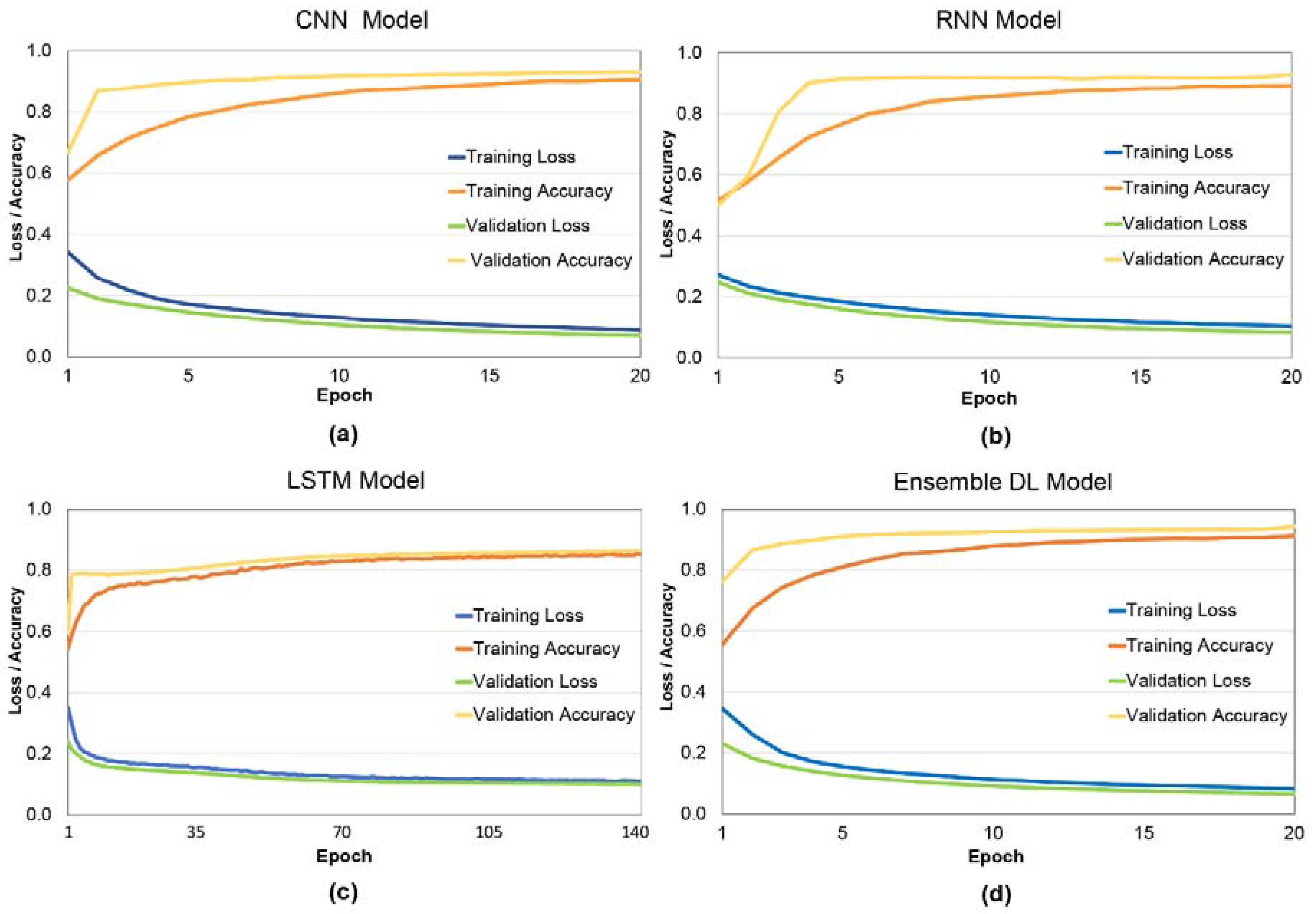
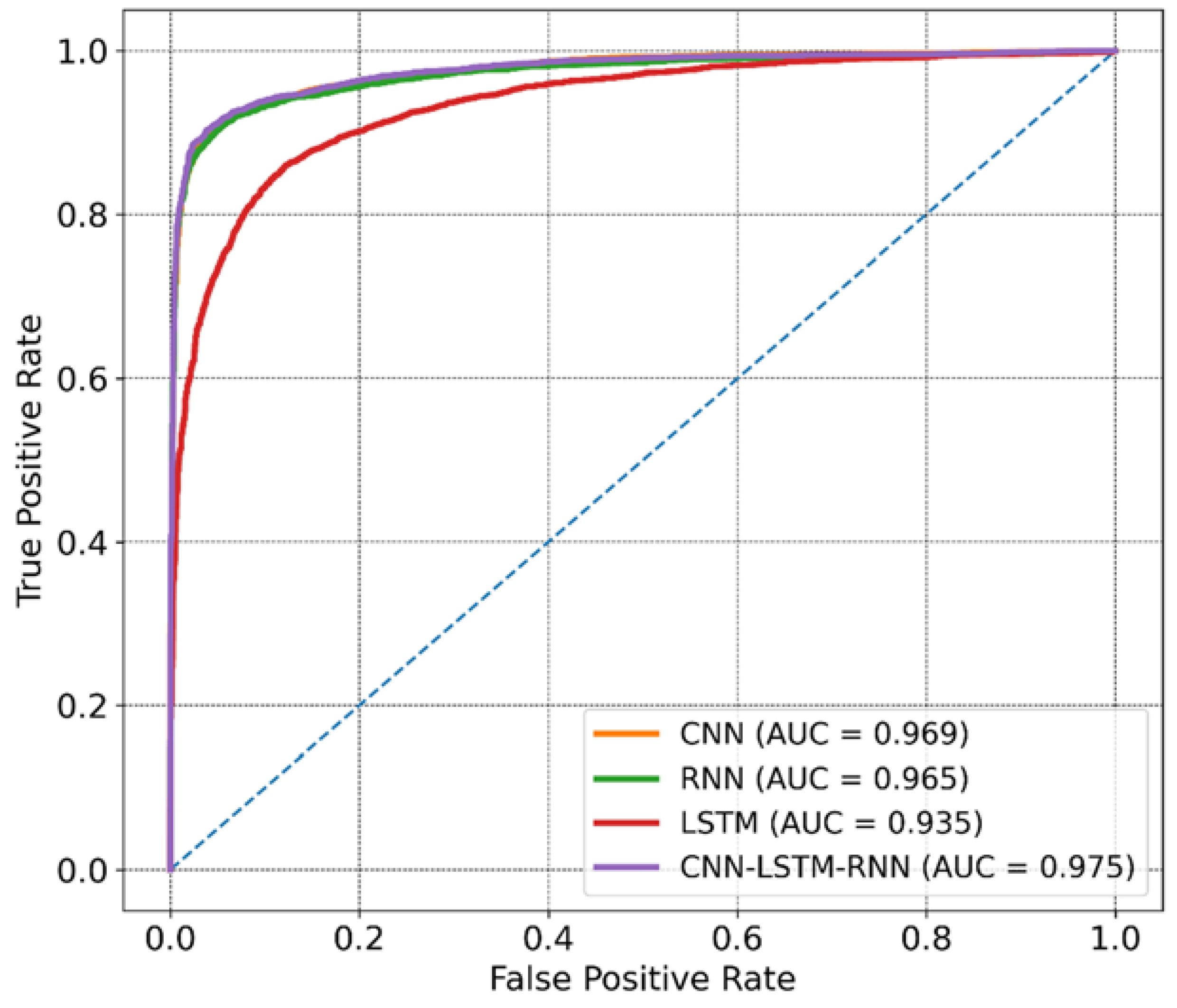
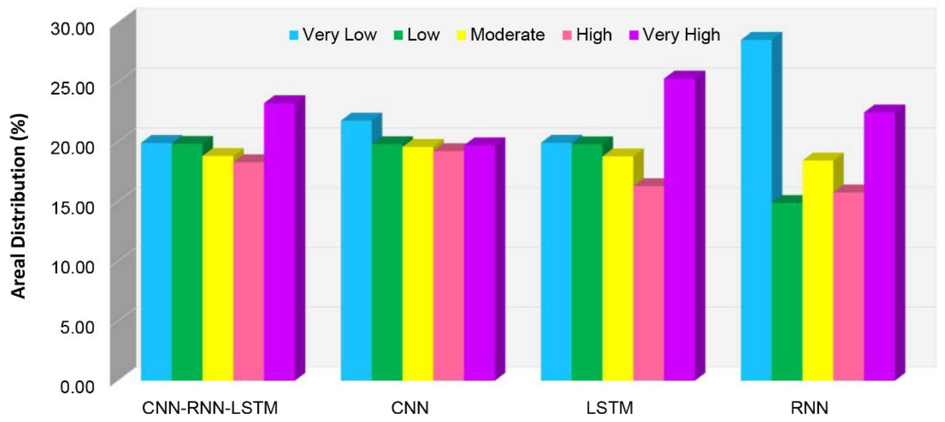
DL algorithms inherently have an internal structure that causes difficulty in explaining and interpreting their results. To be more specific, CNNs contain complicated/convoluted statistical designs with non-linear activation functions and several hidden layers, making it challenging to analyze and clarify their estimations [73]. On the other hand, explaining model outputs provides an understanding of which features influences the established model to what extent, discarding irrelevant/unnecessary (if any) factors from the dataset, as well as making more reliable and sound comparisons for the predictive performances of the models. To address and achieve these issues, in this present study, introduced by [74], the SHapley Additive exPlanations (SHAP) approach was adopted to elucidate the DL model output. On a fundamental basis, the SHAP approach is based on game theory to explain the output of learning algorithms more clearly. It provides a unified framework to interpret predictions and a marginal contribution of each feature in a dataset, through calculating the Shapley values that provide the coherence of the explanations. In contrast to the conventional feature importance score operations of existing ML algorithms, the SHAP approach can assess whether a feature contributes adversely or positively to the model performance.

In addition to the SHAP analysis, Wilcoxon signed-ranked test, which is a non-parametric hypothesis test, was also implemented to statistically measure the effectiveness of the produced models. The test has been intensively utilized to quantify the statistical significance of performance differences between models and make a pair-wise comparison [75,76]. The null hypothesis for the Wilcoxon signed-rank test is that there exists no statistical difference between the models at a 95% confidence interval. The prior assumption is rejected if z values surpass the critical threshold value (1.96), and thus, it can be concluded that the differences in the predictive performances of the models are statistically significant.

4. Results

The present work proposed a novel ensemble DL approach based on shared layers architecture to generate LSMs of a case study in the Trabzon. A total of 12 landslide causative factors were employed in the modeling of DL architectures. To implement the proposed strategy, the average merit of each factor was initially estimated using the CFS to conduct an a priori analysis. According to the results, a slope with 0.755 average merit was the most important factor, having the highest importance score, followed by TRI (0.696), slope length (0.329), NDVI (0.300), aspect (0.201), distance to rivers (0.126), TWI (0.113), elevation (0.080), distance to roads (0.061), lithology (0.045), and road density (0.029). These findings are also in harmony with earlier investigations in this region. In fact, it is a well-recognized fact in the literature that slope is one the most significant agents in the initiation of landslide activities. On the other hand, TPI (0.022) was the least effective parameter for predicting landslide susceptibility (Figure 8). The average merits of all explanatory factors were higher than zero, implying that each factor has a meaningful influence on the landslide susceptibility modeling [77]. Therefore, DL model training was performed without discarding any factor from the initial dataset.

The loss function, or the objective function, is represented as the error of the model, which is the difference between empirical and predicted values. The loss values can be reduced by updating the model weights with the backpropagation algorithm. The degree to which the anticipated value is near to the empirical value is referred to as accuracy [53]. The loss and accuracy values were calculated for both model validation and model training state during the training of DL models. Figure 9 depicts the model performances for the aforementioned model parameters in that all DL models performed successfully in correlating the link between training and validation dataset avoiding overfitting. The validation accuracies of the DL models namely, proposed ensemble DL, CNN, RNN, and LSTM were computed as 0.94, 0.93, 0.92, and 0.87, respectively. On the other hand, it was confirmed that both validation and training loss values converge to approximately 0.1. On account of the difference between accuracy and loss values, all models did not overfit and properly estimated the landslide vulnerability to a new dataset.

Assessment of the effectiveness of the applied methods has been recognized as a significant instrument in gathering information about the accuracy of LSMs produced, and the interpretation of these results. To evaluate the predictive performances of four resultant LSMs, six well-known predictive performance evaluation measures (i.e., OA, precision, recall, F1 score, Kappa coefficient, and AUC score) were used. According to the outcomes of performance analysis, the proposed model (i.e., CNN–LSTM–RNN) produced had higher predictive ability in terms of all accuracy measures compared to the single DL algorithms (i.e., CNN, RNN, and LSTM) (

Table 3. Predictive performances of single and proposed ensemble DL algorithms.

DL Model	Prediction Result
	OA	Precision	Recall	F1 Score	Kappa	AUC	Time (sec.)
RNN	0.91	0.93	0.89	0.91	0.83	0.969	21.04
CNN	0.92	0.95	0.89	0.92	0.84	0.965	25.06
LSTM	0.86	0.86	0.86	0.86	0.73	0.935	402.00
CNN–LSTM–RNN	0.93	0.96	0.91	0.93	0.86	0.975	61.17

). To be more specific, the CNN–LSTM–RNN model had the highest predictive performance of 0.93, whilst the RNN produced results with 0.92, followed by the CNN (0.91) and the LSTM (0.86), in terms of overall accuracy.

The receiver operating characteristic (ROC) curve has been widely employed in assessing the predictive achievement of algorithms, including susceptibility mapping studies, since it allows a visual depiction of the diagnostic performance of a model. The AUC scores range between 0.5 and 1. The predictive performances of the models can be called fair (if the AUC value is between 0.7 and 0.8), good (if the AUC value is in the range 0.8–0.9), or excellent (if the AUC value is between 0.9–1) [78]. Considering the results in this study, the CNN–RNN–LSTM model had the greatest AUC value of 0.975, followed by the CNN (0.969), RNN (0.965), and LSTM (0.935) (Figure 10).

The results clearly showed that the predictive performance of each DL model can be described as excellent. To measure and evaluate the discrepancy between the effectiveness of the models, the Kappa coefficient, commonly utilized to test inter-rater dependability, was also estimated. The Kappa coefficient was estimated as 0.86 for the CNN–RNN–LSTM model whilst the Kappa coefficient of 0.73 was calculated for the LSTM method, indicating substantial agreement between the model and reality.

Apart from the performance assessment metrics, model training times of DL algorithms were also considered to assess their computational complexities. Whilst the LSTM is the model that takes the longest to train with 402.00 s., CNN and RNN networks were completed the model training phase with 21.04 and 25.06 s., respectively. Moreover, the CNN–LSTM–RNN model accomplished its training in approximately one minute. It should be worth mentioning that the proposed shared layers strategy is satisfactory in terms of the model-learning period as well as predictive performances.

In addition to the accuracy assessment metrics, differences between the model performances were statistically measured by using Wilcoxon signed-rank test to make impartial and sound comparisons. If the computed statistical value is higher than the threshold level (1.96 for a 95% confidence interval), it can be said that the difference in model performances is statistically significant. Based on the statistical test results, all estimated statistical values for each model were higher than the critical value (

Table 4. Statistical significance test using Wilcoxon-signed rank test.

	CNN	RNN	LSTM	CNN–LSTM–RNN
CNN	-	7.44	8.12	11.07
RNN		-	2.14	2.62
LSTM			-	4.22
CNN–LSTM–RNN				-

). That is, the results of the statistical significance test clearly revealed that the predictive performance differences among three single DL and the proposed ensemble DL models were statistically significant. In other words, it could be clearly stated that the proposed CNN–LSTM–RNN model produced statistically superior results over the other three single DL models, since the estimated statistical test values were higher than the critical table value.

The SHAP summary graph (Figure 11) ranks the most influential landslide conditioning factors based on their importance, combining local interpretations from the SHAP deep explainer function. In the summary graph, the factors in red color (e.g., slope, TRI, road density, aspect, and elevation) have positive impacts on the model prediction performances, while the factors in blue color (e.g., NDVI) influence the probability of landslide occurrence negatively. Moreover, the size of the scale representing the colors of factors corresponds to feature importance, indicating that the slope was the most influential one among the factors, followed by TRI, road density, aspect, and elevation. When the factors positively contribute to the landslide occurrence, it could be clearly seen that all of them are topographical agents except road density. Moreover, it should be noted that the slope had a positive effect on the model in the 0.63 to 0.90 probabilistic range where the probability of landslide is high, which is consistent with the CFS analysis. On the other hand, the NDVI has negative importance in terms of occurrences of landslides since its values are closer to 1. To be more specific, NDVI had a negative effect on the model in the range of 0.91–0.95, where the probability of landslide is the highest, implying that the NDVI has an inverse contribution in this interval, compared with the slope. The SHAP analysis showed that high NDVI values indicating the dense and healthy vegetation cover had an inverse effect on landslide occurrence. This is a reasonable and acceptable finding considering the ability of densely vegetated areas to reduce the potential risk of mass movements by protecting the land from excessive surface water, supporting drainage, and providing soil stabilization. On the other hand, it can be deduced from the SHAP graph that the increase in the values of the slope would increase the landslide risk. This can be explained by the fact that increasing the gradient of the slope causes the deterioration of slope stability, thus increasing the probability of mass movement activity.

It should be worth mentioning that the natural break approach was adopted to reclassify the generated LSMs into five susceptibility levels (i.e., very low, low, moderate, high, and very high). When the produced LSMs, based on DL models, were visually analyzed, it was obvious that high and very high susceptibility zones were predominantly densified on the central and relatively southeast parts of the study area (Figure 12). Nonetheless, it was found that these zones in the study area were not regularly scattered at the same intensities, but in some regions (e.g., especially center parts), there was a distribution of in the same susceptibility zones. However, the north and northeast parts of the study area are mainly composed of very low and low susceptible zones. The main reason underlying this issue is that the north of the region consists of a coastline where the slope and elevation are generally low. Moreover, given the a priori analysis results obtained by the CFS method, the slope was the most notable parameter in the prediction of landslide susceptibility, confirming that it is plausible and acceptable in this respect.

According to the LSM generated by the proposed ensemble-based DL strategy (i.e., CNN–RNN–LSTM), 19.90%, 19.81%, 18.80%, 18.28%, and 23.22% of the entire area in Trabzon province were considered as having very low, low, moderate, high, and very high landslide susceptibility, respectively (Figure 13). For the CNN algorithm, the very low class had the largest area percentage (21.76%), followed by low (19.79%), very high (19.69%), moderate (19.56%), and high (19.20%). When it comes to the LSTM algorithm, a similar proportional distribution similar to the ensemble DL approach was observed. The highest susceptibility index of LSTM was in the very high (25.28%), followed by very low (19.91%), low (19.78%), moderate (18.77%), and high (16.27%). In the LSM produced by the RNN algorithm, very high, high, moderate, low, and very low landslide susceptibility classes had the 22.44%, 15.75%, 18.42%, 14.87%, and 28.52% percentage areas, respectively. Considering the spatial susceptibility distributions obtained by four methods, these results imply that roughly 20% of the study area consists of very high landslide-susceptible regions.

5. Discussion

The correct identification of landslide hotspot zones and analyzing landslide susceptibility is of utmost significance for decision makers and related public institutions to conduct integrated disaster management and construct emergency action plans. However, in landslide susceptibility mapping studies, several critical issues—such as selection of proper landslide sampling strategy, determination of landslide predisposing factors, and the use of susceptibility modeling approaches—have usually been challenging for researchers, owing to the dynamics and non-linear mechanisms of landslides.

Another encountered problem is related to the errors and inconsistencies resulting from the conversion of inventory and factor maps, particularly from vector maps to raster maps. Some landslide causative factors such as lineaments, road, and river networks are intrinsically represented by lines in vector format. Other parameters, particularly the ones derived from DEM, are represented by grids, referred to as raster format. To process both types of data, vector maps are usually converted into raster format, which is a much easier and more effective way of producing landslide susceptibility maps. In the conversion of landslide inventory maps, a special attention should be paid to the formation of boundary pixels of the polygons representing landslide and non-landslide zones, since these pixels may not have 100% representativeness due to the vector-to-raster conversion process. Inclusion of pixels having some degree of representativeness in reality as 100% representativeness in the inventory map undermines the learning abilities of the model and generalization capabilities. This may provoke pixels outside the landslide polygons, but adjacent to them, to be introduced to the algorithms as if they were a landslide pixel, even though they do not have a 100% landslide risk. For this reason, the correct representation of the inbound boundaries of the landslide zone polygons is of critical importance for the established models to make an accurate estimation. In the current literature, many landslide sampling strategies, namely landslide area, point, scarp, and seed cell, have been proposed to achieve such a critical step [79,80,81]. Their main purpose is to adopt a precise sampling strategy by creating an environment that is entirely representative of the pre-failure circumstances.

In the production of an LSM, one of the most critical and challenging tasks is the determination of optimal landslide contributing factors [82]. In the literature, many contributing factors have been employed for susceptibility mapping. However, the selection of optimal landslide causative factors is still the subject of research, and there are still no globally agreed clear frameworks or guidelines. The main reason for this could be explained by the particular characteristics of study sites under consideration [83]. More specifically, while any factor utilized in LSM may be a contributing factor for a certain area, it may not be for another [49]. On the other side, superfluous and irrelevant contributing factors will diminish the reliability and the predictive accuracy of the algorithm, and thus increase the instability. In the research area, feature selection algorithms, particularly the filter-based ones including CFS, information gain, gain ratio, and Relief-F, have been intensively implemented [84,85,86]. With the application of CFS in the study, it was observed that no factor should be eliminated among the 12 factors. In other words, all 12 factors had a meaningful contribution to the model performance.

A great deal of modeling algorithms for the landslide susceptibility prediction has been proposed and implemented from past to present. For instance, analyzing 565 peer-reviewed articles concerning landslide susceptibility, [87] reported that a total of 163 algorithms were applied for susceptibility zonation in these studies. They also addressed that the use of such a large number of different algorithms also elaborates the comparison of susceptibility models and associated mapping results. On the other hand, which algorithm would offer the most ideal solution to a landslide susceptibility prediction problem is another highly controversial and obscure issue. Under all the above-mentioned circumstances, the production of LSMs through the integration of multiple algorithms with ensemble schemes, rather than deciding on the use of an individual learning algorithm, would be a more appropriate approach. Moreover, the concerns on a model (i.e., generalization and overfitting) can be emerging, necessitating the regularization approach (i.e., ensemble) to the models for eliminating these complications. Besides, generating diversity in extracting the features of the dataset with a single DL model has been a serious issue. The use of ensembling schemes, which can eliminate potentially biased inferences of individual learning algorithms by ensuring diversity within the established model, is rare to find for DL models in the literature, but it has been studied lately for ML algorithms [15,88].

DL algorithms have recently been employed for a broad range of complex problems, including landslide susceptibility mapping [28]. DL architectures have been used to perform computations in several layers instead of a single layer approach and use enormous amounts of data simultaneously. Furthermore, the DL models discover even the parameters to be defined in ML and can be able to produce a superior assessment. Despite their superior performance, one of the most important limitations of DL models is their complication in clarifying the rationale and ensuring corroborating evidence to explain their outputs. Moreover, the necessity of interpretation and explanation of the results from such models limits their comprehensive adoption. Therefore, most of the efforts in the DL community have gone into solving this problem by proposing a series of techniques (i.e., SHAP and LIME) for decision-making processes of learning algorithms. In this study, SHAP analysis results revealed that some landslide predisposing factors had positive (e.g., slope, TRI, road density, aspect, and elevation) or negative (only NDVI) effects on the ensemble DL model proposed in this study. Even though DL algorithms have been intensively utilized for the identification of landslide susceptibility [68,69,89], elucidating the outputs of DL models with such approaches have received limited attention in the literature.

Owing to the nature of landslide susceptibility mapping studies, the use of many thematic variables in a wide range is an inevitable reality. This also engenders the necessity to evaluate contributing factors of different resolutions or scales together. In the study, thematic maps of 11 conditioning factors were available at 30 m resolution and only one factor map (i.e., lithology) was at a scale of 1/100,000, theoretically corresponding to a 20 m resolution. Therefore, 30 m spatial grid resolution was considered as the optimal solution for all parameters to avoid virtual resampling of pixels into 20 m for the 11 thematic maps, at the same time, to protect and process the original pixels values.

6. Conclusions

The intensity and frequency of landslides have become a more serious and harsh problem in Trabzon province, Turkey, due to the climatic conditions, geomorphological agents, and accelerated urban expansion that causes enormous loss of human lives and economic harms. Therefore, the production of reliable and robust LSMs is a tremendous necessity for landslide disaster avoidance and prevention studies. The current work intends to propose a novel ensemble DL strategy based on the shared blocks to boost the landslide prediction accuracies of the single DL models, a mentioned model which integrates CNN, LSTM, and RNN models, all of which were trained using the optimizer of Adagrad. Results of the developed shared layers model, CNN, LSTM, and RNN models were assessed and compared through accuracy assessment and statistical analysis. Some critical implications can be drawn from the outcomes of this work, as follows:

(i) The experimental consequences exhibited the proposed shared layer model (CNN–RNN–LSTM) had the highest prediction accuracy (0.93%), followed by the RNN (0.92%), CNN (0.91%), and LSTM (0.86%) models. Concisely, the suggested model performed approximately 7% better when compared with the LSTM model in terms of OA scores.

(ii) Similar to the other accuracy assessment metrics derived from the confusion matrix, the AUC score of the proposed ensemble DL strategy had the highest AUC score with 0.975, while the LSTM model had the lowest AUC score with 0.935. It can be clearly concluded that the proposed strategy outperformed the single-DL model by about 4% in terms of AUC score.

(iii) To make a more robust comparative analysis, a statistical significance test, Wilcoxon signed-rank test, was applied. The test results revealed that that the differences between the performances of all models were statistically significant at a 95% confidence interval, which once again proved that the ensemble DL model outperformed the single DL models. With the application of the Wilcoxon signed-rank test, the performance differences up to 7% between the proposed ensemble-based DL architecture and the other three individual DL models were not only numerically observed, but also validated statistically.

(iv) The ensemble DL strategy, based on shared blocks, found results in approximately 61 sec. This clearly implies that the training duration of the proposed strategy was approximately 7 times faster than that of the LSTM (402 s), pointing out that the model is also computationally feasible. This finding also implies that the proposed ensemble DL model had an effective and practical architecture in terms of both performance and processing time.

(v) The top three important parameters (i.e., slope, TRI, and slope length) were detected as the factors that represent the geomorphologic characteristics of the study area under investigation. On the other hand, TPI, which is a measure of topographic slope position, was found to be the least effective factor. This information obtained about the landslide predisposing factors with the CFS application, which is considered as a pre-processing step, enabled both the detection of potential factors that will adversely impact the model performance of LSMs and the understanding of which factor contributes to the model performance and to what extent.

(vi) With the application of the SHAP method, factors affecting the model, in which landslide probabilities were higher, were determined. Results revealed that the slope had the highest positive contribution in regions where the probability of landslide occurrence was high, while NDVI had adverse implications. In addition, it is worth mentioning that topographic factors made a significant contribution to the landslide occurrences in the study area, considering that four out of the six most influential parameters on landslide phenomena were slope, TRI, elevation, and aspect.

To sum up, a high accurate LSM is invaluable for facilitating governments with planning the city and preventing/minimizing the effects of landslides. Succeeding extensions of this study might contain the LSM application of the ensemble DL with shared layer architectures using time series datasets, including daily meteorological (i.e., rainfall, wind, and temperature) and remotely sensed datasets (e.g., point clouds and multispectral images). This study revealed the effectiveness and importance of DL models and their ensembled forms in natural disaster impact assessment. For other applications, it is planned not only to evaluate datasets related to different landslide-prone regions, but also to develop more generalized ensemble DL algorithms.

References

1. Tihon, A. Impact of Natural Disasters, Psychological and Physical Effects on the Population. In Abstracts of The Second Eurasian RISK-2020 Conference and Symposium; Aliyev, V., Ed.; AIJR Publisher: Tbilisi, Georgia, 2020; pp. 133–134. [Google Scholar]
2. Lacasse, S.; Nadim, F. Landslide Risk Assessment and Mitigation Strategy. In Bridge Engineering Handbook, 2nd ed.; Springer: Berlin/Heidelberg, Germany, 2009; pp. 315–359. [Google Scholar] [CrossRef]
3. Highland, L.M.; Bobrowsky, P. The Landslide Handbook-A Guide to Understanding Landslides; Kidd, M., Ed.; U.S. Geological Survey Circular 1325: Reston, VA, USA, 2008; p. 129. ISBN 978-141-132-226-4.
4. Pradhan, S.P.; Siddique, T. Mass Wasting: An Overview. Adv. Nat. Technol. Hazards Res. 2019, 50, 3–20. [Google Scholar] [CrossRef]
5. Haque, U.; da Silva, P.F.; Devoli, G.; Pilz, J.; Zhao, B.; Khaloua, A.; Wilopo, W.; Andersen, P.; Lu, P.; Lee, J.; et al. The Human Cost of Global Warming: Deadly Landslides and Their Triggers (1995–2014). Sci. Total Environ. 2019, 682, 673–684. [Google Scholar] [CrossRef]
6. Froude, M.J.; Petley, D.N. Global Fatal Landslide Occurrence from 2004 to 2016. Nat. Hazards Earth Syst. Sci. 2018, 18, 2161–2181. [Google Scholar] [CrossRef] [Green Version]
7. Guha-Sapir, D.; Below, R.; Hoyois, P. EM-DAT: International Disaster Database. Available online: http://www.emdat.be (accessed on 4 October 2021).
8. Dai, F.C.; Lee, C.F.; Ngai, Y.Y. Landslide Risk Assessment and Management: An Overview. Eng. Geol. 2002, 64, 65–87. [Google Scholar] [CrossRef]
9. Guzzetti, F.; Carrara, A.; Cardinali, M.; Reichenbach, P. Landslide Hazard Evaluation: A Review of Current Techniques and Their Application in a Multi-Scale Study, Central Italy. Geomorphology 1999, 31, 181–216. [Google Scholar] [CrossRef]
10. Gómez, H.; Kavzoglu, T. Assessment of Shallow Landslide Susceptibility Using Artificial Neural Networks in Jabonosa River Basin, Venezuela. Eng. Geol. 2005, 78, 11–27. [Google Scholar] [CrossRef]
11. Bijukchhen, S.M.; Kayastha, P.; Dhital, M.R. A Comparative Evaluation of Heuristic and Bivariate Statistical Modelling for Landslide Susceptibility Mappings in Ghurmi-Dhad Khola, East Nepal. Arab. J. Geosci. 2013, 6, 2727–2743. [Google Scholar] [CrossRef]
12. Soeters, R.; Van Westen, C.J. Slope Instability Recognition, Analysis and Zonation. In Landslides: Investigation and Mitigation. Transportation Research Board National Research Council; Special Report No. 247; Turner, K.T., Schuster, R.L., Eds.; National Academy Press: Washington, DC, USA, 1996; pp. 129–177. [Google Scholar]
13. Thiebes, B. Landslide Analysis and Early Warning—Local and Regional Case Study in the Swabian Alb, Germany; Springer: Berlin, Germany, 2012. [Google Scholar]
14. Pradhan, B. A Comparative Study on the Predictive Ability of the Decision Tree, Support Vector Machine and Neuro-Fuzzy Models in Landslide Susceptibility Mapping Using GIS. Comput. Geosci. 2013, 51, 350–365. [Google Scholar] [CrossRef]
15. Hu, X.; Zhang, H.; Mei, H.; Xiao, D.; Li, Y.; Li, M. Landslide Susceptibility Mapping Using the Stacking Ensemble Machine Learning Method in Lushui, Southwest China. Appl. Sci. 2020, 10, 4016. [Google Scholar] [CrossRef]
16. Marjanović, M.; Kovačević, M.; Bajat, B.; Voženílek, V. Landslide Susceptibility Assessment Using SVM Machine Learning Algorithm. Eng. Geol. 2011, 123, 225–234. [Google Scholar] [CrossRef]
17. Kavzoglu, T.; Kutlug Sahin, E.; Colkesen, I. An Assessment of Multivariate and Bivariate Approaches in Landslide Susceptibility Mapping: A Case Study of Duzkoy District. Nat. Hazards 2015, 76, 471–496. [Google Scholar] [CrossRef]
18. Taalab, K.; Cheng, T.; Zhang, Y. Mapping Landslide Susceptibility and Types Using Random Forest. Big Earth Data 2018, 2, 159–178. [Google Scholar] [CrossRef]
19. Pourghasemi, H.R.; Jirandeh, A.G.; Pradhan, B.; Xu, C.; Gokceoglu, C. Landslide Susceptibility Mapping Using Support Vector Machine and GIS at the Golestan Province, Iran. J. Earth Syst. Sci. 2013, 122, 349–369. [Google Scholar] [CrossRef] [Green Version]
20. Merghadi, A.; Abderrahmane, B.; Tien Bui, D. Landslide Susceptibility Assessment at Mila Basin (Algeria): A Comparative Assessment of Prediction Capability of Advanced Machine Learning Methods. ISPRS Int. J. Geo-Inf. 2018, 7, 268. [Google Scholar] [CrossRef] [Green Version]
21. Sahin, E.K. Comparative Analysis of Gradient Boosting Algorithms for Landslide Susceptibility Mapping. Geocarto Int. 2020, 1–25. [Google Scholar] [CrossRef]
22. Can, R.; Kocaman, S.; Gokceoglu, C. A Comprehensive Assessment of XGBoost Algorithm for Landslide Susceptibility Mapping in the Upper Basin of Ataturk Dam, Turkey. Appl. Sci. 2021, 11, 4993. [Google Scholar] [CrossRef]
23. Wang, Y.; Fang, Z.; Hong, H.; Peng, L. Flood Susceptibility Mapping Using Convolutional Neural Network Frameworks. J. Hydrol. 2020, 582, 124482. [Google Scholar] [CrossRef]
24. Bjånes, A.; De La Fuente, R.; Mena, P. A Deep Learning Ensemble Model for Wildfire Susceptibility Mapping. Ecol. Inform. 2021, 65, 101397. [Google Scholar] [CrossRef]
25. Sublime, J.; Kalinicheva, E. Automatic Post-Disaster Damage Mapping Using Deep-Learning Techniques for Change Detection: Case Study of the Tohoku Tsunami. Remote Sens. 2019, 11, 1123. [Google Scholar] [CrossRef] [Green Version]
26. Cui, W.; He, X.; Yao, M.; Wang, Z.; Li, J.; Hao, Y.; Wu, W.; Zhao, H.; Chen, X.; Cui, W. Landslide Image Captioning Method Based on Semantic Gate and Bi-Temporal LSTM. ISPRS Int. J. Geo-Inf. 2020, 9, 194. [Google Scholar] [CrossRef] [Green Version]
27. Kong, W.; Dong, Z.Y.; Jia, Y.; Hill, D.J.; Xu, Y.; Zhang, Y. Short-Term Residential Load Forecasting Based on LSTM Recurrent Neural Network. IEEE Trans. Smart Grid 2019, 10, 841–851. [Google Scholar] [CrossRef]
28. Li, W.; Fang, Z.; Wang, Y. Stacking Ensemble of Deep Learning Methods for Landslide Susceptibility Mapping in the Three Gorges Reservoir Area, China. Stoch. Environ. Res. Risk Assess. 2021, 1–22. [Google Scholar] [CrossRef]
29. Xiao, L.; Zhang, Y.; Peng, G. Landslide Susceptibility Assessment Using Integrated Deep Learning Algorithm along the China-Nepal Highway. Sensors 2018, 18, 4436. [Google Scholar] [CrossRef] [Green Version]
30. Zhong, C.; Liu, Y.; Gao, P.; Chen, W.; Li, H.; Hou, Y.; Nuremanguli, T.; Ma, H. Landslide Mapping with Remote Sensing: Challenges and Opportunities. Int. J. Remote Sens. 2020, 41, 1555–1581. [Google Scholar] [CrossRef]
31. Sameen, M.I.; Pradhan, B.; Lee, S. Application of Convolutional Neural Networks Featuring Bayesian Optimization for Landslide Susceptibility Assessment. Catena 2020, 186, 104249. [Google Scholar] [CrossRef]
32. Chen, H.; Zeng, Z.; Tang, H. Landslide Deformation Prediction Based on Recurrent Neural Network. Neural Process. Lett. 2015, 41, 169–178. [Google Scholar] [CrossRef]
33. Mutlu, B.; Nefeslioglu, H.A.; Sezer, E.A.; Ali Akcayol, M.; Gokceoglu, C. An Experimental Research on the Use of Recurrent Neural Networks in Landslide Susceptibility Mapping. ISPRS Int. J. Geo-Inf. 2019, 8, 578. [Google Scholar] [CrossRef] [Green Version]
34. Wang, Y.; Fang, Z.; Wang, M.; Peng, L.; Hong, H. Comparative Study of Landslide Susceptibility Mapping with Different Recurrent Neural Networks. Comput. Geosci. 2020, 138, 104445. [Google Scholar] [CrossRef]
35. Song, J.; Wang, Y.; Fang, Z.; Peng, L.; Hong, H. Potential of Ensemble Learning to Improve Tree-Based Classifiers for Landslide Susceptibility Mapping. IEEE J. Sel. Top. Appl. Earth Obs. Remote Sens. 2020, 13, 4642–4662. [Google Scholar] [CrossRef]
36. Wang, Y.; Feng, L.; Li, S.; Ren, F.; Du, Q. A Hybrid Model Considering Spatial Heterogeneity for Landslide Susceptibility Mapping in Zhejiang Province, China. Catena 2020, 188, 104425. [Google Scholar] [CrossRef]
37. Ji, J.; Chen, X.; Luo, C.; Li, P. A Deep Multi-Task Learning Approach for ECG Data Analysis. In Proceedings of the 2018 IEEE EMBS International Conference on Biomedical & Health Informatics (BHI), Las Vegas, NV, USA, 4–7 March 2018; pp. 124–127. [Google Scholar] [CrossRef]
38. Yalcin, A. A Geotechnical Study on the Landslides in the Trabzon Province, NE, Turkey. Appl. Clay Sci. 2011, 52, 11–19. [Google Scholar] [CrossRef]
39. Ozturk, K. Landslips and the Effects of These on Turkey. Gazi Univ. J. Gazi Educ. Fac. 2002, 22, 35–50. [Google Scholar]
40. Bayrak, T.; Ulukavak, M. Trabzon Landslides. Electron. J. Map Technol. 2009, 1, 20–30. [Google Scholar]
41. Kavzoglu, T.; Sahin, E.K.; Colkesen, I. Landslide Susceptibility Mapping Using GIS-Based Multi-Criteria Decision Analysis, Support Vector Machines, and Logistic Regression. Landslides 2014, 11, 425–439. [Google Scholar] [CrossRef]
42. Hussin, H.Y.; Zumpano, V.; Reichenbach, P.; Sterlacchini, S.; Micu, M.; van Westen, C.; Bălteanu, D. Different Landslide Sampling Strategies in a Grid-Based Bi-Variate Statistical Susceptibility Model. Geomorphology 2016, 253, 508–523. [Google Scholar] [CrossRef]
43. Yilmaz, I. The Effect of the Sampling Strategies on the Landslide Susceptibility Mapping by Conditional Probability and Artificial Neural Networks. Environ. Earth Sci. 2010, 60, 505–519. [Google Scholar] [CrossRef]
44. Xu, C.; Dai, F.; Xu, X.; Lee, Y.H. GIS-Based Support Vector Machine Modeling of Earthquake-Triggered Landslide Susceptibility in the Jianjiang River Watershed, China. Geomorphology 2012, 145–146, 70–80. [Google Scholar] [CrossRef]
45. Süzen, M.L.; Doyuran, V. A Comparison of the GIS Based Landslide Susceptibility Assessment Methods: Multivariate versus Bivariate. Environ. Geol. 2004, 45, 665–679. [Google Scholar] [CrossRef]
46. Dou, J.; Paudel, U.; Oguch, T.; Uchiyama, S.; Hayakavva, Y.S. Shallow and Deep-Seated Landslide Differentiation Using Support Vector Machines: A Case Study of the Chuetsu Area, Japan. Terr. Atmos. Ocean. Sci. 2015, 26, 227–239. [Google Scholar] [CrossRef] [Green Version]
47. Yalcin, A.; Reis, S.; Aydinoglu, A.C.; Yomralioglu, T. A GIS-Based Comparative Study of Frequency Ratio, Analytical Hierarchy Process, Bivariate Statistics and Logistics Regression Methods for Landslide Susceptibility Mapping in Trabzon, NE Turkey. Catena 2011, 85, 274–287. [Google Scholar] [CrossRef]
48. Colkesen, I.; Sahin, E.K.; Kavzoglu, T. Susceptibility Mapping of Shallow Landslides Using Kernel-Based Gaussian Process, Support Vector Machines and Logistic Regression. J. Afr. Earth Sci. 2016, 118, 53–64. [Google Scholar] [CrossRef]
49. Kavzoglu, T.; Kutlug Sahin, E.; Colkesen, I. Selecting Optimal Conditioning Factors in Shallow Translational Landslide Susceptibility Mapping Using Genetic Algorithm. Eng. Geol. 2015, 192, 101–112. [Google Scholar] [CrossRef]
50. Teke, A.; Kavzoglu, T. Determination of Effective Predisposing Factors Using Random Forest-Based Gini Index in Landslide Susceptibility Mapping. In Proceedings of the 2nd International Geoinformation Days (IGD), Mersin, Turkey, 6 May 2021. [Google Scholar]
51. Chen, W.; Zhang, S.; Li, R.; Shahabi, H. Performance Evaluation of the GIS-Based Data Mining Techniques of Best-First Decision Tree, Random Forest, and Naïve Bayes Tree for Landslide Susceptibility Modeling. Sci. Total Environ. 2018, 644, 1006–1018. [Google Scholar] [CrossRef] [PubMed]
52. Ioffe, S.; Szegedy, C. Batch Normalization: Accelerating Deep Network Training by Reducing Internal Covariate Shift. In Proceedings of the 32nd International Conference Machine Learning, Lille, France, 6–11 July 2015; Volume 1, pp. 448–456. [Google Scholar]
53. Goodfellow, I.; Bengio, Y.; Courville, A. Deep Learning; MIT Press: Cambridge, MA, USA, 2016; ISBN 978-0-262-03561-3. [Google Scholar]
54. Huang, F.; Zhang, J.; Zhou, C.; Wang, Y.; Huang, J.; Zhu, L. A Deep Learning Algorithm Using a Fully Connected Sparse Autoencoder Neural Network for Landslide Susceptibility Prediction. Landslides 2020, 17, 217–229. [Google Scholar] [CrossRef]
55. Szandała, T. Review and Comparison of Commonly Used Activation Functions for Deep Neural Networks. In Bio-Inspired Neurocomputing; Springer: Singapore, 2021; pp. 203–224. ISBN 9789811554957. [Google Scholar]
56. Zhang, X.; Pun, M.O.; Liu, M. Semi-supervised Multi-temporal Deep Representation Fusion Network for Landslide Mapping from Aerial Orthophotos. Remote Sens. 2021, 13, 548. [Google Scholar] [CrossRef]
57. Tan, F.; Yu, J.; Jiao, Y.Y.; Lin, D.; Lv, J.; Cheng, Y. Rapid Assessment of Landslide Risk Level Based on Deep Learning. Arab. J. Geosci. 2021, 14, 1–10. [Google Scholar] [CrossRef]
58. Ragab, M.G.; Abdulkadir, S.J.; Aziz, N.; Al-Tashi, Q.; Alyousifi, Y.; Alhussian, H.; Alqushaibi, A. A Novel One-Dimensional Cnn with Exponential Adaptive Gradients for Air Pollution Index Prediction. Sustainability 2020, 12, 10090. [Google Scholar] [CrossRef]
59. Wang, Y.; Wang, X.; Jian, J. Remote Sensing Landslide Recognition Based on Convolutional Neural Network. Math. Probl. Eng. 2019, 2019, 8389368. [Google Scholar] [CrossRef]
60. LeCun, Y.; Bottou, L.; Bengio, Y.; Haffner, P. Gradient-Based Learning Applied to Document Recognition. Proc. IEEE 1998, 86, 2278–2323. [Google Scholar] [CrossRef] [Green Version]
61. Yi, Y.; Zhang, Z.; Zhang, W.; Jia, H.; Zhang, J. Landslide Susceptibility Mapping Using Multiscale Sampling Strategy and Convolutional Neural Network: A Case Study in Jiuzhaigou Region. Catena 2020, 195, 104851. [Google Scholar] [CrossRef]
62. Mezaal, M.R.; Pradhan, B.; Sameen, M.I. Optimized Neural Architecture for Automatic Landslide Detection from High-Resolution Airborne Laser Scanning Data. Appl. Sci. 2017, 7, 730. [Google Scholar] [CrossRef] [Green Version]
63. Niu, X.; Ma, J.; Wang, Y.; Zhang, J.; Chen, H.; Tang, H. A Novel Decomposition-Ensemble Learning Model Based on Ensemble Empirical Mode Decomposition and Recurrent Neural Network for Landslide Displacement Prediction. Appl. Sci. 2021, 11, 4684. [Google Scholar] [CrossRef]
64. Mou, L.; Ghamisi, P.; Zhu, X.X. Deep Recurrent Neural Networks for Hyperspectral Image Classification. IEEE Trans. Geosci. Remote Sens. 2017, 55, 3639–3655. [Google Scholar] [CrossRef] [Green Version]
65. Wang, H.; Zhang, L.; Luo, H.; He, J.; Cheung, R.W.M. AI-Powered Landslide Susceptibility Assessment in Hong Kong. Eng. Geol. 2021, 288, 106103. [Google Scholar] [CrossRef]
66. Pradhan, B. Landslide Susceptibility Mapping of a Catchment Area Using Frequency Ratio, Fuzzy Logic and Multivariate Logistic Regression Approaches. J. Indian Soc. Remote Sens. 2010, 38, 301–320. [Google Scholar] [CrossRef]
67. Lee, S.; Choi, J. Landslide Susceptibility Mapping Using GIS and the Weight-of-Evidence Model. Int. J. Geogr. Inf. Sci. 2004, 18, 789–814. [Google Scholar] [CrossRef]
68. Nhu, V.H.; Hoang, N.D.; Nguyen, H.; Ngo, P.T.T.; Thanh Bui, T.; Hoa, P.V.; Samui, P.; Tien Bui, D. Effectiveness Assessment of Keras Based Deep Learning with Different Robust Optimization Algorithms for Shallow Landslide Susceptibility Mapping at Tropical Area. Catena 2020, 188, 104458. [Google Scholar] [CrossRef]
69. Mandal, K.; Saha, S.; Mandal, S. Applying Deep Learning and Benchmark Machine Learning Algorithms for Landslide Susceptibility Modelling in Rorachu River Basin of Sikkim Himalaya, India. Geosci. Front. 2021, 12, 101203. [Google Scholar] [CrossRef]
70. Qiu, X.; Zhang, L.; Ren, Y.; Suganthan, P.; Amaratunga, G. Ensemble Deep Learning for Regression and Time Series Forecasting. In Proceedings of the 2014 IEEE Symposium on Computational Intelligence in Ensemble Learning, Orlando, FL, USA, 9–12 December 2014; pp. 1–6. [Google Scholar] [CrossRef]
71. Fan, C.; Matkovic, K.; Hauser, H. Sketch-Based Fast and Accurate Querying of Time Series Using Parameter-Sharing LSTM Networks. IEEE Trans. Vis. Comput. Graph. 2020, 27, 4495–4506. [Google Scholar] [CrossRef]
72. Takahashi, R.; Matsubara, T.; Uehara, K. A Novel Weight-Shared Multi-Stage CNN for Scale Robustness. IEEE Trans. Circuits Syst. Video Technol. 2019, 29, 1090–1101. [Google Scholar] [CrossRef]
73. Yap, M.; Johnston, R.L.; Foley, H.; MacDonald, S.; Kondrashova, O.; Tran, K.A.; Nones, K.; Koufariotis, L.T.; Bean, C.; Pearson, J.V.; et al. Verifying Explainability of a Deep Learning Tissue Classifier Trained on RNA-Seq Data. Sci. Rep. 2021, 11, 1–12. [Google Scholar] [CrossRef]
74. Lundberg, S.M.; Lee, S.I. A Unified Approach to Interpreting Model Predictions. Adv. Neural Inf. Process. Syst. 2017, 30, 4766–4775. [Google Scholar]
75. Pham, B.T.; Jaafari, A.; Prakash, I.; Bui, D.T. A Novel Hybrid Intelligent Model of Support Vector Machines and the MultiBoost Ensemble for Landslide Susceptibility Modeling. Bull. Eng. Geol. Environ. 2019, 78, 2865–2886. [Google Scholar] [CrossRef]
76. Sahin, E.K.; Colkesen, I.; Kavzoglu, T. A Comparative Assessment of Canonical Correlation Forest, Random Forest, Rotation Forest and Logistic Regression Methods for Landslide Susceptibility Mapping. Geocarto Int. 2020, 35, 341–363. [Google Scholar] [CrossRef]
77. Thai Pham, B.; Tien Bui, D.; Prakash, I. Landslide Susceptibility Modelling Using Different Advanced Decision Trees Methods. Civ. Eng. Environ. Syst. 2018, 35, 139–157. [Google Scholar] [CrossRef]
78. Cantor, S.B.; Kattan, M.W. Determining the area under the ROC curve for a binary diagnostic test. Med. Decis. Mak. 2000, 20, 468–470. [Google Scholar] [CrossRef]
79. Nefeslioglu, H.A.; Gokceoglu, C.; Sonmez, H. An Assessment on the Use of Logistic Regression and Artificial Neural Networks with Different Sampling Strategies for the Preparation of Landslide Susceptibility Maps. Eng. Geol. 2008, 97, 171–191. [Google Scholar] [CrossRef]
80. Dou, J.; Yunus, A.P.; Merghadi, A.; Shirzadi, A.; Nguyen, H.; Hussain, Y.; Avtar, R.; Chen, Y.; Pham, B.T.; Yamagishi, H. Different Sampling Strategies for Predicting Landslide Susceptibilities Are Deemed Less Consequential with Deep Learning. Sci. Total Environ. 2020, 720, 137320. [Google Scholar] [CrossRef]
81. Dagdelenler, G.; Nefeslioglu, H.A.; Gokceoglu, C. Modification of Seed Cell Sampling Strategy for Landslide Susceptibility Mapping: An Application from the Eastern Part of the Gallipoli Peninsula (Canakkale, Turkey). Bull. Eng. Geol. Environ. 2016, 75, 575–590. [Google Scholar] [CrossRef]
82. Yalcin, A. GIS-Based Landslide Susceptibility Mapping Using Analytical Hierarchy Process and Bivariate Statistics in Ardesen (Turkey): Comparisons of Results and Confirmations. Catena 2008, 72, 1–12. [Google Scholar] [CrossRef]
83. Van Westen, C.J.; Rengers, N.; Soeters, R. Use of Geomorphological Expert Knowledge in Indirect Landslide Hazard Assessment. Nat. Hazards 2003, 30, 399–419. [Google Scholar] [CrossRef]
84. Pham, B.T.; Vu, V.D.; Costache, R.; Van Phong, T.; Ngo, T.Q.; Tran, T.H.; Nguyen, H.D.; Amiri, M.; Tan, M.T.; Trinh, P.T.; et al. Landslide Susceptibility Mapping Using State-of-the-Art Machine Learning Ensembles. Geocarto. Int. 2021, 1–25. [Google Scholar] [CrossRef]
85. Tanyu, B.F.; Abbaspour, A.; Alimohammadlou, Y.; Tecuci, G. Landslide Susceptibility Analyses Using Random Forest, C4.5, and C5.0 with Balanced and Unbalanced Datasets. Catena 2021, 203, 105355. [Google Scholar] [CrossRef]
86. Abedini, M.; Ghasemian, B.; Shirzadi, A.; Shahabi, H.; Chapi, K.; Pham, B.T.; Bin Ahmad, B.; Tien Bui, D. A Novel Hybrid Approach of Bayesian Logistic Regression and Its Ensembles for Landslide Susceptibility Assessment. Geocarto Int. 2019, 34, 1427–1457. [Google Scholar] [CrossRef]
87. Reichenbach, P.; Rossi, M.; Malamud, B.D.; Mihir, M.; Guzzetti, F. A Review of Statistically-Based Landslide Susceptibility Models. Earth-Sci. Rev. 2018, 180, 60–91. [Google Scholar] [CrossRef]
88. Dou, J.; Yunus, A.P.; Bui, D.T.; Merghadi, A.; Sahana, M.; Zhu, Z.; Chen, C.W.; Han, Z.; Pham, B.T. Improved Landslide Assessment Using Support Vector Machine with Bagging, Boosting, and Stacking Ensemble Machine Learning Framework in a Mountainous Watershed, Japan. Landslides 2020, 17, 641–658. [Google Scholar] [CrossRef]
89. Van Dao, D.; Jaafari, A.; Bayat, M.; Mafi-Gholami, D.; Qi, C.; Moayedi, H.; Van Phong, T.; Ly, H.B.; Le, T.T.; Trinh, P.T.; et al. A Spatially Explicit Deep Learning Neural Network Model for the Prediction of Landslide Susceptibility. Catena 2020, 188, 104451. [Google Scholar] [CrossRef]
Figure 1. Study area and landslide locations.
Remotesensing 13 04776 g001
Figure 2. Lithological structure of the study area.
Remotesensing 13 04776 g002
Figure 3. Flowchart of the adopted methodology in the study.
Remotesensing 13 04776 g003
Figure 4. The units of a simple RNN: The RNN unit is a type of looping design that allows for the continuation of information (ht−1) connected to previous knowledge (ht).
Remotesensing 13 04776 g004
Figure 5. The units of a simple LSTM: A typical LSTM unit carries out and controls information using three gates: input (it), forget (ft), and output gates (ot).
Remotesensing 13 04776 g005
Figure 6. Concept of shared layers’ structure.
Remotesensing 13 04776 g006
Figure 7. The shared layers ensemble architectures.
Remotesensing 13 04776 g007
Figure 8. Importance scores of conditioning factors, obtained by correlation-based feature selection.
Remotesensing 13 04776 g008
Figure 9. The learning curve, including training loss/accuracy values and validation loss/accuracy values of the individual and ensemble DL models. (a) CNN model, (b) RNN model, (c) LSTM model, and (d) ensemble DL model.
Remotesensing 13 04776 g009
Figure 10. The area under the receiver operating curve analysis for produced DL models.
Remotesensing 13 04776 g010
Figure 11. SHAP graph for the most effective conditioning factors.
Remotesensing 13 04776 g011
Figure 12. Landslide susceptibility maps produced by (a) CNN, (b) RNN, (c) LSTM, and (d) CNN–LSTM–RNN.
Remotesensing 13 04776 g012
Figure 13. Areal distribution of each susceptibility class for CNN, LSTM, RNN, and ensemble DL models.
Remotesensing 13 04776 g013