Building Function Mapping Using Multisource Geospatial Big Data: A Case Study in Shenzhen, China

Abstract

Building function labelling plays an important role in understanding human activities inside buildings. This study develops a method of function label classification using integrated features derived from remote sensing and crowdsensing data with an extreme gradient boosting tree (XGBoost). The classification framework is verified based on a dataset from Shenzhen, China. An extended label system for six building types (residential, commercial, office, industrial, public facilities, and others) was applied, and various social functions were considered. The overall classification accuracies were 88.15% (kappa index = 0.72) and 85.56% (kappa index = 0.69). The importance of features was evaluated using the occurrence frequency of features at decision nodes. In the six-category classification system, the basic building attributes (22.99%) and POIs (46.74%) contributed most to the classification process; moreover, the building footprint (7.40%) and distance to roads (11.76%) also made notable contributions. The result shows that it is feasible to extract building environments from POI labels and building footprint geometry with a dimensional reduction model using an autoencoder. Additionally, crowdsensing data (e.g., POI and distance to roads) will become increasingly important as classification tasks become more complicated and the importance of basic building attributes declines.

1. Introduction

With the development of sensors and computational techniques, many urban studies have modelled cities as diverse and fine-scale spatial units including functional zones [1,2], blocks [3,4], and buildings [5,6]. Different scale levels provide various perspectives for understanding a city. When deconstructing a city into a set of landscape components, buildings are among the most common units [7,8,9,10,11]. A natural spatial object/unit/segmentation scheme that bridges the spatial scale from the macrolevel (e.g., urban level) to the microlevel (e.g., individual level) can be established [12,13]. As a type of population hub, buildings are structures where many human activities occur. These human activities can be in turn classified based on the characteristics of the building where they occur [14]. Among all building characteristics, building type is one of the most commonly used, since it provides a categorical label and corresponding semantic information, which can be leveraged to infer the human activities that occur in the corresponding buildings.

Building-type data are widely used in assessments of human activities. Buildings account for the largest energy consumption in the economy [15], and many researchers utilized building-type data to estimate energy consumption and understand energy demand patterns across different building types [16,17]. With increasing requests for high spatial–temporal resolution population mapping [18,19], building-type data has been leveraged for population mapping [20,21]. Additionally, such data has also been introduced into the studies of urban planning [22], housing demand [23], and urban noise exposure [24]. Building-type data are typically collected and maintained by local authorities, who rely on large-scale field surveys. Since the data collection process is time-consuming and labor-intensive, the availability of building-type data is severely limited in terms of the spatial coverage and temporal resolution. To address this issue, recent studies have explored methods of generating building types from data with satisfactory spatiotemporal coverage and affordability. Most existing studies have used remote sensing data (e.g., nighttime light data [25]), crowdsensing data (e.g., points of interest (POIs) [26], trajectory data [27,28], and street view photos [29,30]), and their hybrids [5]. (1) The remote sensing approach involves building footprint identification, in which pixel-based text and spectral information are retrieved and later leveraged to identify building objects (geometry) and obtain building-type labels. Super-high spatial/spectral resolution data, e.g., light detection and ranging (LiDAR) data [29,31], are typically used to enhance the spatial/spectral resolution of features and their derived footprint. However, it is challenging to distinguish buildings with different socioeconomic functions (e.g., a restaurant and a bank) but similar spectral characteristics. Moreover, the high price of high-resolution images may limit the use of such images as a nationwide survey measure for building types. (2) In the crowdsensing approach, socioeconomic data with spatial tags can be used to classify various buildings based on social characteristics (e.g., neighboring POIs) even if their physical characteristics (spectral and geometric) are similar. However, some crowdsensing data (e.g., traffic trajectory and street view data) may be limited, because of privacy issues, or unavailable for many cities [5].

This paper proposes an integrated building classification method using extreme gradient boosting (XGBoost) to generate function-oriented building-type labels and overcome the above challenges. XGBoost, a widely utilized implementation of a gradient boosted regression tree (GBRT), has displayed state-of-the-art performance in many machine learning tasks, such as classification [32]. Both remote sensing (land surface temperature and nighttime light data) and crowdsensing (POIs, building footprints, and roads) data are used to distinguish buildings with different socioeconomic functions, but high-resolution remote sensing images are excluded to improve algorithm applicability for large-scale surveys.

2. Materials and Methods

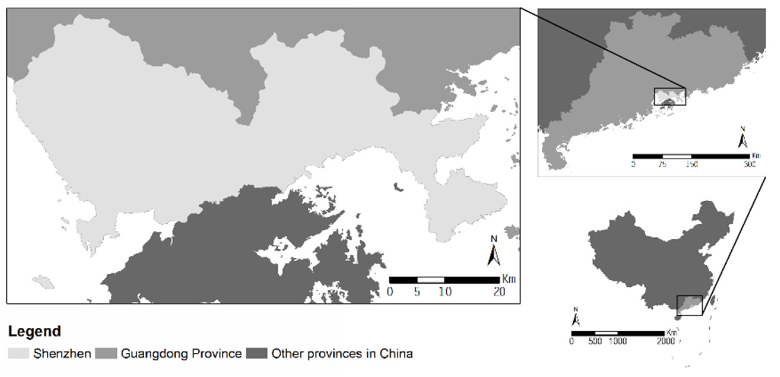
2.1. Study Area

Shenzhen became the first special economic zone in China in 1980. This megacity is located in the Pearl River Delta and had a population of approximately 13.44 million in late 2019; additionally, Shenzhen is one of the largest and wealthiest cities in China. The highly developed city has a large number of buildings with diverse function types. Thus, Shenzhen is selected as the study area, and the location of Shenzhen is shown in Figure 1.

2.2. Data Collection

To identify buildings and classify ambient environment information, five datasets (building datasets, points of interest (POIs), road networks, nighttime light (NTL) data, and land surface temperature (LST) products) are included in this study. All datasets mentioned above covered Shenzhen, China, and were collected in 2015.

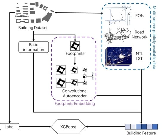
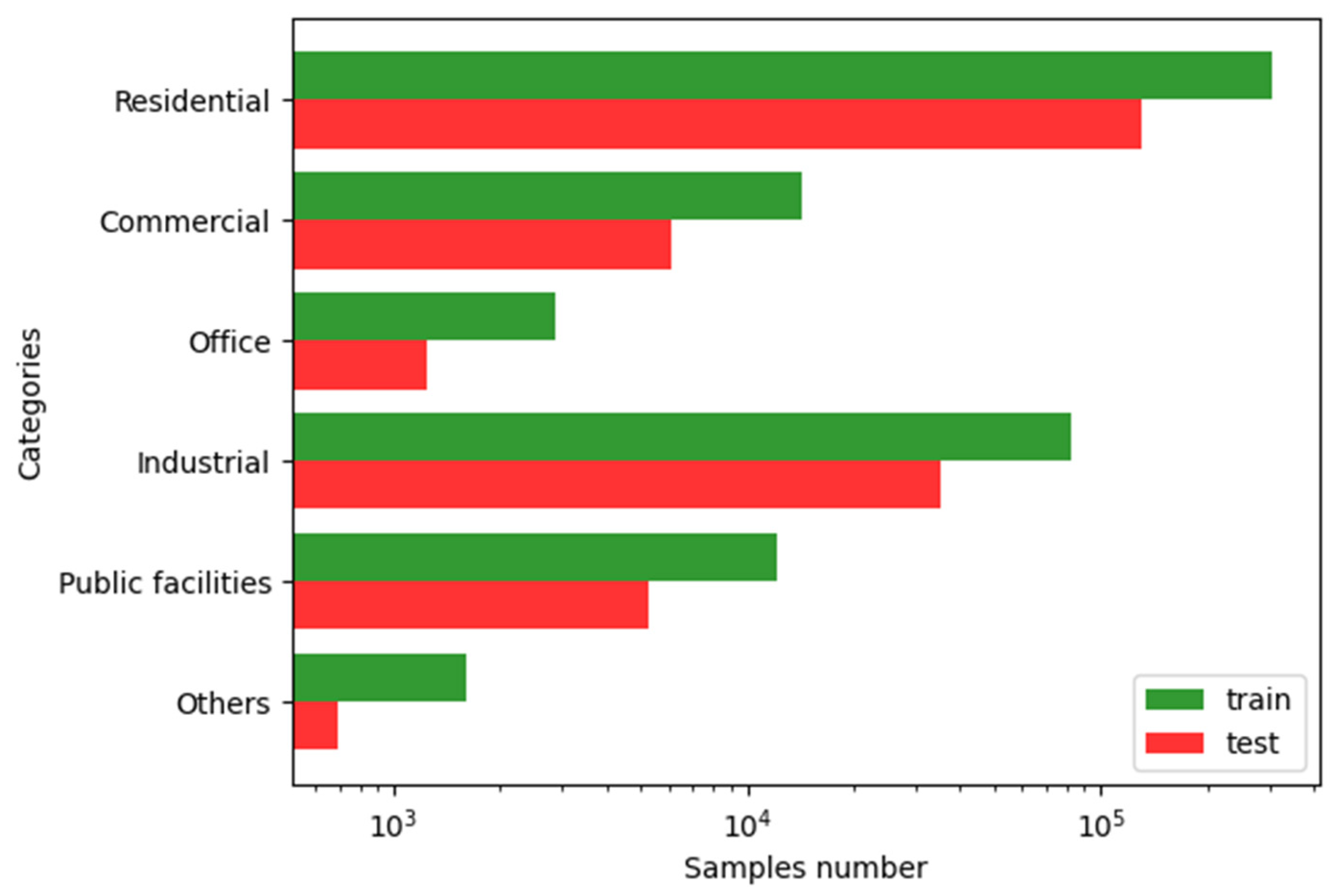
• The building dataset contains 599,457 buildings. A manually labelled building class is provided for each building. The building height, perimeter, area, floor area ratio, and lowest/highest floor number are also recorded. The building footprint geometry is recorded in polygon format in an ArcGIS shapefile.
• The POI dataset includes 991,362 POIs in Shenzhen, China. The dataset was retrieved from Gaode Map (https://lbs.amap.com/api/webservice/guide/, accessed on 19 January 2021), one of the most popular map platforms in China, and the POIs are labelled with 20 primary classifications and 984 secondary classifications.
• The road network dataset, including 109,551 road links, was collected from OpenStreetMap (OSM), a collaborative open-source map project. The roads in the OSM (https://wiki.openstreetmap.org/wiki/Key:highway, accessed on 19 January 2021) dataset are labelled based on 74 categories and reclassified into 13 categories: motorway, primary, secondary, tertiary, trunk, track, ordinary road, residential, cycleway, path, service road, linking road, and unclassified road. The distance from a building to the nearest road of each type is calculated and used as a proxy to represent the ambient road network. The location of a building is generally related to its use, and the distance to various kinds of roads can represent the ambient road network. For instance, residential buildings are usually close to residential roads, and industrial buildings are usually near trunk roads for transportation purposes.
• For the NTL dataset, we use an annual product (Annual VNL V2) based on a cloud-free day–night band (DNB) composite from Visible Infrared Imaging Radiometer Suite (VIIRS). The gridded image aggregating yearly NTL in 2015 is downloaded from the website of Earth Observation Group (https://eogdata.mines.edu/products/vnl/, accessed on 19 January 2021). The spatial resolution of the image is 500 × 500 m². The pixels where a building is located are directly retrieved as the NTL features for a building.
• The LST images with spatial resolution of 0.05 deg/pixel are from a monthly Moderate Resolution Imaging Spectroradiometer (MODIS) product (MYD11C3v006) which is publicly available on the NASA EarthData site (https://lpdaac.usgs.gov/products/myd11c3v006/, accessed on 19 January 2021). Eight images are used, including the monthly average daytime and nighttime land surface temperatures in January, April, September, and October 2015. Each building is assigned a digital number (DN) based on that of the nearest pixel to the centroid point for a given building.

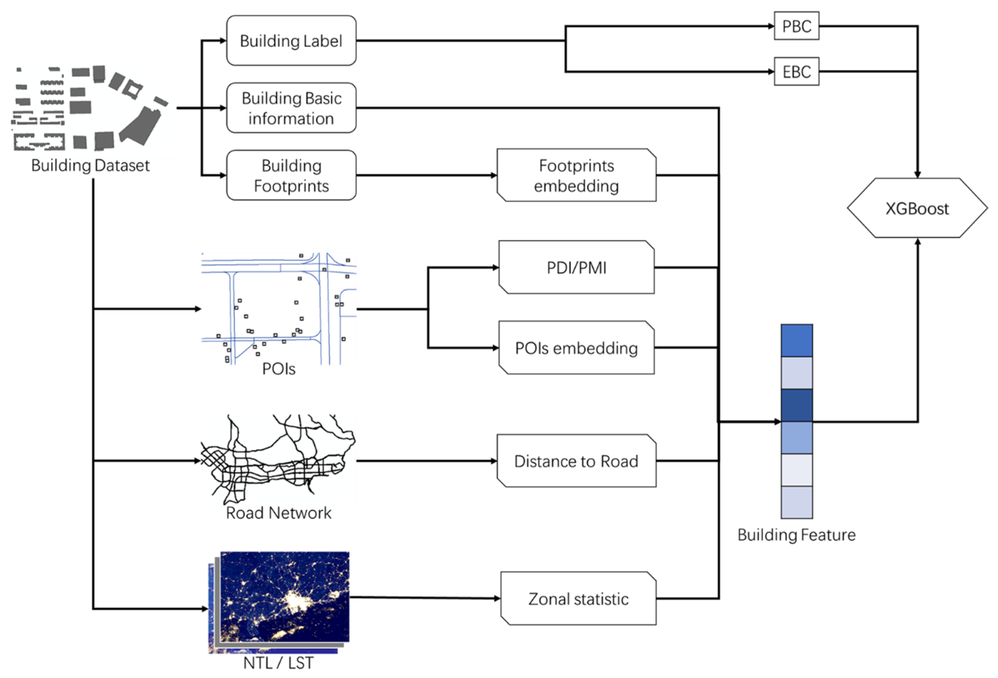
2.3. Methodology

An integrated building-type classification method is proposed and applied to predict the primary building categories (PBC) and the extended building categories (EBC). A set of features (basic building information, POIs, the road network, NTL data, and LSTs) are extracted for each building. In particular, the extracted sparse (POI) and high-dimensional (building footprint vectors rasterized as 2D images) features are compressed using autoencoder networks (Figure 2) and later involved in the XGBoost process.

2.3.1. Building Label

A building is manually labelled with a PBC and EBC. The PBC includes six major building categories: residential, commercial, office, industrial, public facilities, and others; based on the PBC, the EBC includes 19 finer building types, such as residential buildings, residential support facilities, shopping malls, restaurants, hotels, office buildings, industrial buildings, warehouses, schools, traffic, and public support facilities. The completed categories in PBC and EBC are listed in

Table 1. Primary and extended building category.

PBC	EBC	Description
Residential	Residential buildings	Buildings for residential usage
	Residential support facilities	Supporting facilities (e.g., power distribution, pump, and guard buildings)
Commercial	Super-specialty stores	Large stores selling furniture, clothing, and sporting goods
	Commercial streets	Streets with stores alongside it
	Shopping malls	Large indoor shopping centers
	Restaurants	Buildings providing food service
	Hotels	Buildings providing hotel service
	Other stores	Other buildings for commercial usage
Office	Office buildings	Buildings for office usage
Industrial	Industrial buildings	Factories and buildings for industrial usage
	Warehouses	Buildings for storing goods
Public facilities	Schools	Nurseries, kindergartens, primary and secondary schools, higher vocational schools, universities
	Medical buildings	Medical centers, hospitals, clinics, and medical emergency centers
	Sports	Stadiums, gyms, and sports clubs
	Subway	Subway stations
	Railway	Railway stations
	Traffic	Other traffic facilities
	Public support facilities	Municipal facilities and community support facilities
Others	Others	Other buildings

, as well as their descriptions. Specially, an EBC is adopted to determine whether the proposed model can distinguish detailed differences in socioeconomic function among each primary class. The labels were generated by filtering the buildings by their addresses with a set of given keywords (e.g., cuisine and restaurants for the “restaurant” class). The labels were later corrected manually. The observations were subsequently weighted based on their labels, as shown in Equation (1). $W_j$ is the weight for all samples with label $j$, $N$ is the total number of samples (buildings), $k$ is the number of labels, and $N_j$ is the number of labels $j$.

$$W_j=N/\left(k\ast N_j\right)$$

(1)

2.3.2. Building Features

For each building, five groups of features (basic building information, POIs, the road network, NTL data, and LSTs) are constructed, including 38 features in total (

Table 2. Extracted features for building classification.

Source	Features	Dimension	Descriptions
Basic building information	Basic attributes	6	Building height (m), perimeter (m), area (m2), floor area ratio, lowest/highest floor number 1
	Footprint embedding	4	Compressed presentation of the building footprint
POIs	POI embedding	4	Compressed presentation of POIs
	POI index	2	PDI and PMI
Road network information	Distance to roads	13	Distance to the nearest road (by type)
Nighttime light value		1	Annually averaged NTL value
Land surface temperature		8	Daytime and nighttime land surface temperatures in January, April, September, and October.

¹ Including the number of floors in the underground part of the building.

). Among these attributes, the POI and footprint features are generated using two autoencoder networks introduced in the following section. Two indices, namely, the POI density index (PDI) and the POI mixture index (PMI), are calculated from Equations (3) and (4). All other attributes are directly retrieved from the input dataset.

The building footprint geometry is important in identifying the building class. The geometry is typically recorded as a vector of 2D points, and this vector cannot be directly applied in the XGBoost algorithm. Thus, these geometries are projected to a raster. An autoencoder is later built to extract a feature vector and obtain a compressed representation. Theses extracted 1D feature vectors can be later used in the XGBoost algorithm directly. An autoencoder is a neural network that minimizes the difference between the input(s) and output; by doing so, the output of the middle layer (compressed representation) can represent the input in a reduced dimension [33,34]. An autoencoder consists of two parts: a reduction network and a reconstruction network. The reduction network encodes the input into a reduced representation, and the reconstruction network generates an output that is as close to the input as possible, based on the corresponding encoding. Due to the advantages of sparse interactions and parameter sharing, convolutional layers are adopted in the autoencoder [33].

Figure 3 shows the flowchart used to encode the building footprints. To embed the building footprints into a vector, raster images with 256 × 256 pixels are generated from the building footprint geometry. The raster images are used to train a convolutional-based autoencoder. Finally, the encoder network is used to embed each building footprint into a four-dimensional vector.

POI data have been widely used to measure urban vibrancy and detect urban functional zones [35,36]. Usually, a high density of POIs indicates high urban vibrancy, and various functional areas are associated with different categories of POIs. For urban functional zone classification, the functional categories can be derived directly based on the POIs inside a given zone since it covers a large enough number of POIs. However, the area of a building is much smaller than a functional zone, which means the number of POIs in most buildings is too limited to derive their categories. Moreover, the usage of two buildings can be different even though their major POI categories are the same. For example, inside both office buildings and commercial buildings, commercial POIs are the most commonly seen POIs. Therefore, we extract the nearby POIs and embed these POIs into a vector to describe the nearby functional area context for each building.

In the dataset, one POI has at least one label based on the service provided, and we encode a POI $p$ using a sparse vector $v_p={\left[v_p{}^{\left(1\right)},v_p{}^{\left(2\right)},\dots \right]}^T$. The value $v_p{}^{\left(i\right)}$ is 1 when $p$ is classified in the $i$-th category; otherwise, the value is 0. For building $b$, the neighbor POI set $P_b$ contains the POIs within a certain distance threshold (e.g., 500 m). By summing the POI vectors of all POIs in $P_b$, we obtain a POI vector for building $b$ by weighted sum:

$$v_b=\frac{{\sum }_{p\in P_b}{w}_{b, p}{v}_p}{{\sum }_{p\in P_b}{w}_{b, p}}.$$

(2)

Here, we consider the connection intensity between the building $b$ and a POI $p$ by introducing a weight $w_{b, p}$, which can be determined by the distance between them. In this study, the weights for POIs within a close distance (e.g., 200 m) are set as 1, and inverse distance weight (IDW) is adopted to calculate the weights for other POIs with a further distance. Before obtaining the weight by IDW, the bias will be first subtracted from the distance so that the weights are consistent spatially.

Based on the neighboring POI set, the PDI and PMI can be calculated as two features for classification. The PDI is calculated by counting the number of POI labels among neighbors, and the PMI is the Shannon entropy value calculated based on the POI vector of a building:

$$PD{I}_b=\left|P_b\right|,$$

(3)

$$PM{I}_b=-{\tilde{v}}_b{}^T\log \left({\tilde{v}}_b\right),$$

(4)

where ${\tilde{v}}_b$ is the normalized $v_b$ variable, such that the sum of the elements in ${\tilde{v}}_b$ equals 1. The elemental logarithmic function is denoted as $\log$. Specially, we define $\log \left(0\right)=0$.

Moreover, considering the sparseness of the high-dimensional POIs vector, an autoencoder with three fully connected hidden layers is built to embed the POI vector for building $v_b$ into a vector with a reduced dimension. The first and last hidden layers share the same output shape, and the output of the most internal layer $z_b$ has a much smaller dimension. Finally, $z_b$ is taken as the embedding vector used for classification.

2.3.3. Extreme Gradient Boosting (XGBoost)

XGBoost is a widely utilized implementation of a gradient boosted regression tree (GBRT), and it has displayed state-of-the-art performance in many machine learning tasks [32]. In XGBoost models, normalization of inputs is not required due to the characteristics of the regression trees, and regularization is applied to prevent overfitting. Considering the above advantages, XGBoost is adopted as the classifier in this study.

Given a dataset $D$ with $n$ samples, each sample has $m$ features. Let $s_i=\left(x_i,y_i\right)$ represent the $i$-th sample in the dataset $D$. Here, $x_i$ is an $m$-dimensional vector of features, and $y_i$ is the labelled category. For a feature vector $x_i$, a tree ensemble model with $T$ independent regression trees can predict an output:

$${\widehat{y}}_i=\varphi \left(x_i\right)={\sum }_{t=1}^T{f}_t\left(x_i\right),$$

(5)

where $f_t$ is the $t$-th regression tree. The objective of learning the above model is to minimize the following regularized loss function:

$$ℒ\left(\varphi \right)={\sum }_{i=1}^n\ell \left({\widehat{y}}_i,y_i\right)+{\sum }_{t=1}^T\mathsf{\Omega }\left(f_t\right),$$

(6)

where $l$ denotes a loss function related to the difference between the predicted and actual labels, and $\mathrm{\Omega }$ is a regularization function used to evaluate the complexity of the model. The regularization term is designed to avoid overfitting.

In the tree ensemble model, it is difficult to minimize the loss function $L$ using conventional optimization methods, so gradient boosting is commonly applied in GBRT. Gradient boosting is a greedy algorithm that uses gradient methods to optimize the objective and generates the $\left(t+1\right)$-th tree based on the $t$-th tree. Compared to ordinary GBRT, which only considers the first-order gradient, a second-order approximation is used in XGBoost. In addition, shrinkage and column subsampling are also included in XGBoost to prevent overfitting.

2.3.4. Accuracy Assessment

To evaluate the performance of the model, the confusion matrix is calculated based on the predicted and actual labels of samples in the test dataset. Suppose there are $K$ categories in total; let $C_{K\times K}$ denote the confusion matrix for a given test sample set. The element $c_{i,j}$ in matrix $C$ is the number of observed samples in category $i$ and predicted samples in category $j$. Based on the confusion matrix, the overall accuracy (OA; $p_o$) and kappa ($\kappa$) values can be calculated to evaluate the model using the following equations:

$$p_o=\frac{{\sum }_{k=1}^K{c}_{k,k}}{{\sum }_{c\in C}c},$$

(7)

$$ℒ\kappa =\frac{p_o-p_e}{1-p_e},$$

(8)

$$p_e=\frac{{\sum }_{k=1}^K\left({\sum }_{i=1}^K{c}_{i,k}{\sum }_{j=1}^K{c}_{k,j}\right)}{{\left({\sum }_{c\in C}c\right)}^2}.$$

(9)

3. Results

As discussed in the previous section, we extract the function labels and features for each building. The function labels included two regimes: an PBC directly derived from a manually labelled dataset and an EBC, as shown in

Table 3. (a). Classification performance for the PBC system based on the test dataset. (b). Classification performance for the EBC system.

(a)
PBC	Precision	Recall	F1	Support
Office	49.23%	22.97%	31.33%	1245
Industrial	76.02%	86.74%	81.03%	35,517
Commercial	55.79%	29.04%	38.20%	5557
Others	70.22%	39.39%	50.47%	886
Residential	93.80%	93.56%	93.68%	131,502
Public facility	58.20%	47.36%	52.22%	5131
(b)
EBC	Precision	Recall	F1	Support
Commercial street	45.45%	14.49%	21.98%	69
Hotel	42.03%	11.74%	18.35%	494
Industrial buildings	73.69%	87.88%	80.16%	34,353
Medical	60.71%	37.90%	46.67%	314
Office building	45.04%	25.54%	32.60%	1245
Other stores	52.59%	36.89%	43.36%	4321
Others	66.67%	40.18%	50.14%	886
Railway	62.50%	47.62%	54.05%	21
Residential building	93.15%	93.63%	93.39%	125,867
Restaurants	30.89%	5.18%	8.88%	1138
School	62.36%	38.55%	47.65%	1564
Shopping mall	60.00%	15.79%	25.00%	19
Sport	56.00%	28.00%	37.33%	50
Subway	84.38%	47.37%	60.67%	57
Super-specialty store	100.00%	40.00%	57.14%	10
Support facilities (residential)	40.06%	26.47%	31.88%	5141
Support facilities (public)	49.07%	41.86%	45.18%	2697
Traffic 1	64.09%	27.10%	38.10%	428
Warehousing	44.98%	23.11%	30.53%	1164

¹ Transportation facility’s exclude railway and subway stations.

a,b. The labels are imbalanced, and their Shannon equitability (EH) indexes equal 0.46 and 0.35, respectively. To improve the classification performance for minority building types, the dataset is weighted using Equation (1), where building types with low occurrence are assigned high weights. The features include basic building attributes, building footprints, LSTs, NTL data, distance to roads, and POI features for each building. Among them, the building footprint and POI attributes are compressed using an autoencoder. Originally a 2D vector, the building footprint is first rasterized as a 256 × 256 image and later compressed as a 1D vector (namely, the compressed representation of the building footprint). The trained autoencoder can preserve most of the information from the building footprint in the compressed representation (Acc = 0.9878, F1 = 0.9852, IoU = 0.5581). The POI features are initially recorded as a sparse array (sparseness = 0.8632) [37] with 984 elements (type labels). The raw POI features are later compressed as an array, with four elements retaining most information (RMSE = 0.0003). The dataset (599,457 building observations) is divided into 100 parts, according to the latitude of the area (i.e., rectangular areas equidistant from north to south) where a building is located. Thirty-four consecutive divided areas are randomly selected as the test area, and the remaining areas are used as the training area. An XGBoost tree is later trained based on the training dataset and evaluated based on the test dataset. As Figure 4 shows, the distribution of building types in the training set and test set are similar.

The proposed integrated building classification method yielded 88.15% (kappa index = 0.72) and 85.56% (kappa index = 0.69) overall accuracy values for the PBC and EBC, respectively (Figure 5). The overall accuracy and kappa index decreased as the classification of building types became increasingly complicated. In both classification systems, the building types with high occurrence frequencies (e.g., residential buildings) yielded a high accuracy (93.56% recall), even though the buildings were weighted by type to overcome the class imbalance issue.

The importance of one feature is evaluated based on the frequency of occurrence and information gain at split points (also called decision nodes) in the trained XGBoost tree (

Table 4. Feature importance in building classification.

Feature Type	PBC	EBC
Footprint perimeter	2.11%	1.29%
Height	5.74%	3.46%
Area	1.62%	2.13%
Floor area ratio	1.78%	1.19%
Lowest floor number	0.94%	1.26%
Highest floor number	10.80%	7.97%
Distance to roads	11.76%	12.34%
NTL	1.02%	1.04%
LST	10.10%	11.70%
Compressed POI representation	46.74%	50.18%
Compressed building footprint representation	7.40%	7.44%

). A high occurrence frequency or information gain implies greater importance for a given feature than for others [38,39]. This feature, in this case, is more frequently used to distinguish samples of different building types. Overall, the importance of compressed POI representation and basic building information (footprint perimeter, height, area, floor area ratio, and number of floors) are dominant, with classification contributions at 46.74% and 22.99% information, respectively. The compressed representation of the building footprint (7.40%) and distance to roads (11.76%) also notably contributed to the classification result.

When using PBC, the building features (basic information and building footprint) contribute to classification at approximately 30.39% of the information in the decision tree. In contrast, the ambient environment (POI, NTL, LST, and distance to roads) contributes to classification at 69.61% of information. When EBC is used, the importance of the ambient environment increases to 75.25%, and the importance of building features decreases, except for the compressed representation of the building footprint. This result can be assessed from two perspectives. From one perspective, the ambient socioeconomic environment, especially POI information, plays a key role in differentiating buildings with similar physical characteristics but disparate socioeconomic functions (e.g., a school and an office). From another perspective, conventional building attributes (e.g., height, area, and footprint perimeter) may oversimplify the building footprint geometry as a shape.

The recall values are relatively low in some functional categories, such as hotels, restaurants, and offices. On one hand, buildings in these categories do not have some unique physical features, so they could not be well detected based on the basic attributes and footprints of the buildings. On the other hand, the used POIs, road network, and low-resolution remote sensing data can only reflect rough land usage near a building, so it is a difficult task to figure out the function of a tiny building. Many studies conduct building classification and gain a relatively high accuracy by using expensive data such as Taxi GPS trajectory data, social media data, and very high-resolution (VHR) remote sensing images [27,28,40]. However, these data are expensive and not accessible by the public. It should be noted that in this study, the features for classification are only based on the publicly available data so as to classify a large number of buildings at a very low cost. Compared to some previous studies using publicly available data only [41,42], and even some including VHR images and mobility data [5,25], the proposed method has gained relatively satisfying results for such a difficult task based on data with limited quality.

With the same extracted features, we applied other classifiers implemented by a Python module scikit-learn [43], namely multilayer perception (MLP), decision tree (DT), and random forest (RF), so as to compare the performance of various classifiers. As

Table 5. Performance of various classifiers.

Classifier	PBC		EBC
	OA	Kappa	OA	Kappa
MLP	81.80%	0.53	79.00%	0.49
DT	80.90%	0.55	78.25%	0.54
RF	87.47%	0.68	85.17%	0.66
XGBoost	88.15%	0.72	85.56%	0.69

shows, in terms of the features in this study, tree models gain better results than MLP and SVM, especially the ensemble models. Besides, the boosting model (XGBoost) also performs better than the bagging model (RF).

4. Discussion

Building-type labels provide significant semantic information for understanding the spatial context of human activities. As a function label, building type is widely used as a fundamental input in constructing type-wise models in fields such as energy consumption prediction [44], human mobility mapping [45], urban land surface construction, climate modelling [45], and health outcome evaluation [46]. However, building-type labels are unavailable in many regions, especially at large scales (e.g., the city level). Manually generating building types is labor-intensive and challenging when cities with millions of buildings are experiencing high-speed development. This study thus proposes an integrated classification method using an XGBoost tree. Remote sensing data (LST and NTL data) and crowdsensing data (basic building information, building footprints, distance to roads, and POIs) are jointly used to label the buildings based on their function.

The advantages of the proposed classification method are threefold. First, this study labels buildings with detailed social functions. Buildings with similar physical features but disparate social functions, such as restaurants and stores, are distinguished. Hence, this taxonomic approach groups building types with consistent characteristics (e.g., human mobility patterns). Second, compressed presentations of POIs are built using an autoencoder, and a conversion from a POI category system to a building-type system is achieved. This conversion process allows us to update or predict the changes in building usage in a city when a new POI dataset is renewed (typically annually) in large cities in China. Third, a set of building footprint compressed representations is built using an autoencoder, which can preserve most of the original footprint information (Acc = 0.9878, F1 = 0.9852, and IoU = 0.5581) in a vector with four elements. Conventionally, morphological features are used for footprint embedding. For example, [41] uses five morphological features (conners number, shape index, squareness, elongation, and courtyards number) to describe a building footprint shape. We compare the footprint embedding methods by conducting classification tasks based on six groups of features. In each group, the features consist of basic attributes and footprints features extracted by different methods. Using a Python module named momepy [47], five dimensional morphologic features (the same as [41]) are included in the first group, and 11 more types of morphologic indicators are extracted to formulate the second group of features with 18 dimensions. The footprint features in the rest of the groups are extracted by autoencoders with various embedding dimensions. The results listed in

Table 6. Classification results by XGBoost with various footprints features.

Footprint Features	PBC		EBC
	OA	Kappa	OA	Kappa
Morphologic (5 Dimensions)	73.14%	0.45	67.90%	0.41
Morphologic (18 Dimensions)	75.30%	0.48	71.08%	0.45
Autoencoder (4 Dimensions)	73.38%	0.46	68.52%	0.42
Autoencoder (8 Dimensions)	75.58%	0.48	71.60%	0.45
Autoencoder (16 Dimensions)	76.24%	0.49	72.68%	0.46
Autoencoder (32 Dimensions)	77.00%	0.49	73.65%	0.47

show that features extracted by autoencoder lead to a better accuracy compared to the morphological features with an approximate dimension. It can also be found that a result based on a higher dimension is higher than that based on a lower one. Therefore, compared with conventional building-shape measurements, the compressed representation generated by the autoencoder exhibits more potential in extracting the key characteristics of the footprint geometry.

POI data are widely used as an alternative for depicting urban environments. This study, however, finds POI data to be biased. From one perspective, POI data focus on popular, publicly accessible facilities with high commercial value while overlooking other areas. For instance, the POI densities within commercial, industrial, and public facility building areas are 5001.19, 1857.20, and 3250.39 per km², respectively. The POI density in the commercial building area is three times that in the industrial building area. Over 31.24% of commercial building footprints contained at least one POI after spatially joining the POI points, but these percentages for public facilities and industrial buildings were only 12.53% and 16.58%, respectively. Consequently, the urban landscape representation is biased if only POI data are considered. However, this bias can be corrected by jointly using building-type and footprint data. From another perspective, the area where a building is located has a high chance of being characterized as a commercially popular POI (e.g., a restaurant) if frequently recorded. Although the majority of buildings serve other functions (e.g., offices), the POI oversampling issue may lead to the misclassification of the major building function and the corresponding spatial units. The findings should be considered in the context of some assumptions and limitations. First, building features may vary across countries, or even cities. This study includes one city, Shenzhen, due to the availability of building data. The classification method could be more robust if more data covering more cities were available. Second, the buildings are individually labelled in this study. Buildings with mixed usage (e.g., a shopping mall with restaurants inside) might be misclassified to some extent. Although mixed building types can be approximately represented by a multiclass probability vector, a multilabel approach would provide a more intuitive understanding of buildings in the real world. Third, similar to the spatial patterns of neighboring buildings, other factors may contribute to building classification but are not considered in this study. Fourth, the building footprint data used in the proposed classification process can be expensive to obtain and available in only a limited area if generated manually. This issue will limit the application of our approach in large-scale scenarios (e.g., national scale). However, some extensive studies have provided building footprint identification methods that are cheap and provide high accuracy [48]. Moreover, some commercial building footprint products (e.g., AW3D for global high-resolution 3D map building) can also be employed.

5. Conclusions

Building function labels play a significant role in understanding the urban environment. The corresponding data are, however, severely limited by their availability due to the high time consumption and labor intensity of the data collection process. Thus, it is of great importance to predict or generate building function labels using high-availability and low-cost data. To achieve this objective, two XGBoost tree classifiers were trained in this study to predict the function labels of buildings using the physical and social characteristics of the buildings. The current findings suggest that the XGBoost tree classifier can feasibly classify different taxa (PBC and EBC). Moreover, crowd-sensed data, especially POI data, are found to be dominant in distinguishing buildings with similar social functions. However, this study only considers single-labelled building functions, and the proposed methodology could be extended to mixed usage in the future. In summary, the proposed method provides a convenient way to classify large-scale urban building environments. The generated building-type dataset can be used in urban environment analyses in public health, urban planning, and energy policy development.

References

1. Yuan, N.J.; Zheng, Y.; Xie, X.; Wang, Y.; Zheng, K.; Xiong, H. Discovering urban functional zones using latent activity trajectories. IEEE Trans. Knowl. Data Eng. 2014, 27, 712–725. [Google Scholar] [CrossRef]
2. Gao, S.; Janowicz, K.; Couclelis, H. Extracting urban functional regions from points of interest and human activities on location-based social networks. Trans. GIS 2017, 21, 446–467. [Google Scholar] [CrossRef]
3. Voltersen, M.; Berger, C.; Hese, S.; Schmullius, C. Object-based land cover mapping and comprehensive feature calculation for an automated derivation of urban structure types at block level. Remote Sens. Environ. 2014, 154, 192–201. [Google Scholar] [CrossRef]
4. Song, Y.; Long, Y.; Wu, P.; Wang, X. Are all cities with similar urban form or not? Redefining cities with ubiquitous points of interest and evaluating them with indicators at city and block levels in China. Int. J. Geogr. Inf. Sci. 2018, 32, 2447–2476. [Google Scholar] [CrossRef]
5. Niu, N.; Liu, X.; Jin, H.; Ye, X.; Liu, Y.; Li, X.; Chen, Y.; Li, S. Integrating multi-source big data to infer building functions. Int. J. Geogr. Inf. Sci. 2017, 31, 1871–1890. [Google Scholar] [CrossRef]
6. Hoffmann, E.J.; Wang, Y.; Werner, M.; Kang, J.; Zhu, X.X. Model Fusion for Building Type Classification from Aerial and Street View Images. Remote Sens. 2019, 11, 1259. [Google Scholar] [CrossRef] [Green Version]
7. Saito, K.; Spence, R. Mapping urban building stocks for vulnerability assessment–preliminary results. Int. J. Digit. Earth 2011, 4, 117–130. [Google Scholar] [CrossRef]
8. Chen, Y.; Liu, X.; Li, X.; Liu, X.; Yao, Y.; Hu, G.; Xu, X.; Pei, F. Delineating urban functional areas with building-level social media data: A dynamic time warping (DTW) distance based k-medoids method. Landsc. Urban Plan. 2017, 160, 48–60. [Google Scholar] [CrossRef]
9. Liu, Y.; Wang, W.; Ghadimi, N. Electricity load forecasting by an improved forecast engine for building level consumers. Energy 2017, 139, 18–30. [Google Scholar] [CrossRef]
10. Newsham, G.R.; Birt, B.J. Building-level occupancy data to improve ARIMA-based electricity use forecasts. In Proceedings of the 2nd ACM Workshop on Embedded Sensing Systems for Energy-Efficiency in Building, Zurich, Switzerland, 2 November 2010; pp. 13–18. [Google Scholar]
11. Xing, H.; Meng, Y. Integrating landscape metrics and socioeconomic features for urban functional region classification. Comput. Environ. Urban Syst. 2018, 72, 134–145. [Google Scholar] [CrossRef]
12. Wegener, M. From macro to micro—How much micro is too much? Transp. Rev. 2011, 31, 161–177. [Google Scholar] [CrossRef]
13. Zhou, Y.; Lau, B.P.L.; Yuen, C.; Tunçer, B.; Wilhelm, E. Understanding urban human mobility through crowdsensed data. IEEE Commun. Mag. 2018, 56, 52–59. [Google Scholar] [CrossRef] [Green Version]
14. Liu, Y.; Meng, Q.; Zhang, J.; Zhang, L.; Jancso, T.; Vatseva, R. An effective Building Neighborhood Green Index model for measuring urban green space. Int. J. Digit. Earth 2016, 9, 387–409. [Google Scholar] [CrossRef]
15. International Energy Agency. Directorate of Sustainable Energy Policy. Transition to Sustainable Buildings: Strategies and Opportunities to 2050; Organization for Economic: Paris, France, 2013. [Google Scholar]
16. Robinson, C.; Dilkina, B.; Hubbs, J.; Zhang, W.; Guhathakurta, S.; Brown, M.A.; Pendyala, R.M. Machine learning approaches for estimating commercial building energy consumption. Appl. Energy 2017, 208, 889–904. [Google Scholar] [CrossRef]
17. Yu, Z.; Fung, B.C.M.; Haghighat, F.; Yoshino, H.; Morofsky, E. A systematic procedure to study the influence of occupant behavior on building energy consumption. Energy Build. 2011, 43, 1409–1417. [Google Scholar] [CrossRef] [Green Version]
18. Lloyd, C.T.; Sorichetta, A.; Tatem, A.J. High resolution global gridded data for use in population studies. Sci. Data 2017, 4, 170001. [Google Scholar] [CrossRef] [PubMed] [Green Version]
19. Smith, A.; Bates, P.D.; Wing, O.; Sampson, C.; Quinn, N.; Neal, J. New estimates of flood exposure in developing countries using high-resolution population data. Nat. Commun. 2019, 10, 1814. [Google Scholar] [CrossRef] [PubMed] [Green Version]
20. Ural, S.; Hussain, E.; Shan, J. Building population mapping with aerial imagery and GIS data. Int. J. Appl. Earth Obs. Geoinf. 2011, 13, 841–852. [Google Scholar] [CrossRef]
21. Yao, Y.; Liu, X.; Li, X.; Zhang, J.; Liang, Z.; Mai, K.; Zhang, Y. Mapping fine-scale population distributions at the building level by integrating multisource geospatial big data. Int. J. Geogr. Inf. Sci. 2017, 31, 1220–1244. [Google Scholar] [CrossRef]
22. Gago, E.J.; Roldan, J.; Pacheco-Torres, R.; Ordóñez, J. The city and urban heat islands: A review of strategies to mitigate adverse effects. Renew. Sustain. Energy Rev. 2013, 25, 749–758. [Google Scholar] [CrossRef]
23. Barrios García, J.A.; Rodríguez Hernández, J.E. Housing demand in Spain according to dwelling type: Microeconometric evidence. Reg. Sci. Urban Econ. 2008, 38, 363–377. [Google Scholar] [CrossRef]
24. Thacher, J.D.; Poulsen, A.H.; Raaschou-Nielsen, O.; Jensen, A.; Hillig, K.; Roswall, N.; Hvidtfeldt, U.; Jensen, S.S.; Levin, G.; Valencia, V.H.; et al. High-resolution assessment of road traffic noise exposure in Denmark. Environ. Res. 2020, 182, 109051. [Google Scholar] [CrossRef] [PubMed]
25. Sritarapipat, T.; Takeuchi, W. Building classification in Yangon City, Myanmar using Stereo GeoEye images, Landsat image and night-time light data. Remote Sens. Appl. Soc. Environ. 2017, 6, 46–51. [Google Scholar] [CrossRef]
26. Rahman, M.M.; Avtar, R.; Ahmad, S.; Inostroza, L.; Misra, P.; Kumar, P.; Takeuchi, W.; Surjan, A.; Saito, O. Does building development in Dhaka comply with land use zoning? An analysis using nighttime light and digital building heights. Sustain. Sci. 2021, 16, 1323–1340. [Google Scholar] [CrossRef]
27. Zhuo, L.; Shi, Q.; Zhang, C.; Li, Q.; Tao, H. Identifying building functions from the spatiotemporal population density and the interactions of people among buildings. ISPRS Int. J. Geo-Inf. 2019, 8, 247. [Google Scholar] [CrossRef] [Green Version]
28. Zhong, C.; Huang, X.; Arisona, S.M.; Schmitt, G.; Batty, M. Inferring building functions from a probabilistic model using public transportation data. Comput. Environ. Urban Syst. 2014, 48, 124–137. [Google Scholar] [CrossRef]
29. Srivastava, S.; Vargas-Muñoz, J.E.; Swinkels, D.; Tuia, D. Multilabel Building Functions Classification from Ground Pictures using Convolutional Neural Networks. In Proceedings of the 2nd ACM SIGSPATIAL International Workshop on AI for Geographic Knowledge Discovery, Seattle, WA, USA, 6 November 2018; pp. 43–46. [Google Scholar]
30. Kang, J.; Körner, M.; Wang, Y.; Taubenböck, H.; Zhu, X.X. Building instance classification using street view images. ISPRS J. Photogramm. Remote Sens. 2018, 145, 44–59. [Google Scholar] [CrossRef]
31. Wurm, M.; Taubenbock, H.; Roth, A.; Dech, S. Urban structuring using multisensoral remote sensing data: By the example of the German cities Cologne and Dresden. In Proceedings of the 2009 Joint Urban Remote Sensing Event, Shanghai, China, 20–22 May 2009; pp. 1–8. [Google Scholar]
32. Chen, T.; Guestrin, C. XGBoost: A Scalable Tree Boosting System. In Proceedings of the 22nd ACM SIGKDD International Conference on Knowledge Discovery and Data Mining, San Francisco, CA, USA, 13–17 August 2016; pp. 785–794. [Google Scholar]
33. Goodfellow, I.; Bengio, Y.; Courville, A.; Bengio, Y. Deep Learning; MIT Press: Cambridge, MA, USA, 2016; Volume 1. [Google Scholar]
34. Cheng, Z.; Sun, H.; Takeuchi, M.; Katto, J. Deep convolutional autoencoder-based lossy image compression. In Proceedings of the 2018 Picture Coding Symposium (PCS), San Francisco, CA, USA, 24–27 June 2018; pp. 253–257. [Google Scholar]
35. Hong, Y.; Yao, Y. Hierarchical community detection and functional area identification with OSM roads and complex graph theory. Int. J. Geogr. Inf. Sci. 2019, 33, 1569–1587. [Google Scholar] [CrossRef]
36. Huang, B.; Zhou, Y.; Li, Z.; Song, Y.; Cai, J.; Tu, W. Evaluating and characterizing urban vibrancy using spatial big data: Shanghai as a case study. Environ. Plan. B Urban Anal. City Sci. 2020, 47, 1543–1559. [Google Scholar] [CrossRef]
37. Hoyer, P.O. Non-negative matrix factorization with sparseness constraints. J. Mach. Learn. Res. 2004, 5, 1457–1469. [Google Scholar]
38. Friedman, J.H. Stochastic gradient boosting. Comput. Stat. Data Anal. 2002, 38, 367–378. [Google Scholar] [CrossRef]
39. Hastie, T.; Tibshirani, R.; Friedman, J. The Elements of Statistical Learning. Springer Series in Statistics; Springer: Berlin/Heidelberg, Germany, 2001. [Google Scholar]
40. Xie, J.; Zhou, J. Classification of Urban Building Type from High Spatial Resolution Remote Sensing Imagery Using Extended MRS and Soft BP Network. IEEE J. Sel. Top. Appl. Earth Obs. Remote Sens. 2017, 10, 3515–3528. [Google Scholar] [CrossRef]
41. Steiniger, S.; Lange, T.; Burghardt, D.; Weibel, R. An Approach for the Classification of Urban Building Structures Based on Discriminant Analysis Techniques. Trans. GIS 2008, 12, 31–59. [Google Scholar] [CrossRef]
42. Arunplod, C.; Nagai, M.; Honda, K.; Warnitchai, P. Classifying building occupancy using building laws and geospatial information: A case study in Bangkok. Int. J. Disaster Risk Reduct. 2017, 24, 419–427. [Google Scholar] [CrossRef]
43. Pedregosa, F.; Varoquaux, G.; Gramfort, A.; Michel, V.; Thirion, B.; Grisel, O.; Blondel, M.; Prettenhofer, P.; Weiss, R.; Dubourg, V. Scikit-learn: Machine learning in Python. J. Mach. Learn. Res. 2011, 12, 2825–2830. [Google Scholar]
44. Wei, Y.; Zhang, X.; Shi, Y.; Xia, L.; Pan, S.; Wu, J.; Han, M.; Zhao, X. A review of data-driven approaches for prediction and classification of building energy consumption. Renew. Sustain. Energy Rev. 2018, 82, 1027–1047. [Google Scholar] [CrossRef]
45. Oliveti, M. Analysis of Mobility Patterns in Different Neighbourhoods, Integrating GPS Tracks with OpenStreetMap Data. Master’s Thesis, Delft University of Technology, Delft, The Netherlands, 2015. [Google Scholar]
46. Kwok, Y.T.; De Munck, C.; Schoetter, R.; Ren, C.; Lau, K.K.-L. Refined dataset to describe the complex urban environment of Hong Kong for urban climate modelling studies at the mesoscale. Theor. Appl. Climatol. 2020, 142, 129–150. [Google Scholar] [CrossRef]
47. Fleischmann, M. MOMEPY: Urban morphology measuring toolkit. J. Open Source Softw. 2019, 4, 1807. [Google Scholar] [CrossRef] [Green Version]
48. Dai, Y.; Gong, J.; Li, Y.; Feng, Q. Building segmentation and outline extraction from UAV image-derived point clouds by a line growing algorithm. Int. J. Digit. Earth 2017, 10, 1077–1097. [Google Scholar] [CrossRef]
Figure 1. Study area.
Remotesensing 13 04751 g001
Figure 2. Classification method workflow.
Remotesensing 13 04751 g002
Figure 3. The flowchart of footprint feature embedding.
Remotesensing 13 04751 g003
Figure 4. Samples number of different categories in training set and test set.
Remotesensing 13 04751 g004
Figure 5. Confusion matrix for the test dataset: (a) PBC; (b) EBC.
Remotesensing 13 04751 g005