
Phase Shift Migration with Modified Coherent Factor Algorithm for MIMO-SAR 3D Imaging in THz Band


 ,
,
Abstract
:1. Introduction
2. Theory and Formulation
2.1. Back-Projection Algorithm with Coherence Factor for MIMO-SAR Imaging
2.2. PSM Algorithm for MIMO-SAR Imaging
2.3. Proposed MCF-PSM Algorithm
2.4. Computational Cost
3. Numerical Simulation Results
4. Lab Experiments Results
5. Discussion
6. Conclusions
Author Contributions
Funding
Data Availability Statement
Acknowledgments
Conflicts of Interest
References
- Li, H.; Li, C.; Wu, S.; Zheng, S.; Fang, G. Adaptive 3D Imaging for Moving Targets Based on a SIMO InISAR Imaging System in 0.2 THz Band. Remote Sens. 2021, 13, 782. [Google Scholar] [CrossRef]
- Cheng, B.; Cui, Z.; Lu, B.; Qin, Y.; Liu, Q.; Chen, P.; He, Y.; Jiang, J.; He, X.; Deng, X.; et al. 340-GHz 3-D Imaging Radar With 4Tx-16Rx MIMO Array. IEEE Trans. Terahertz Sci. Technol. 2018, 8, 509–519. [Google Scholar] [CrossRef]
- Zhong, H.; Xu, J.; Xie, X.; Yuan, T.; Reightler, R.; Madaras, E.; Zhang, X.C. Nondestructive defect identification with terahertz time-of-flight tomography. IEEE Sens. J. 2005, 5, 203–208. [Google Scholar] [CrossRef]
- Meo, S.D.; Espín-López, P.F.; Martellosio, A.; Pasian, M.; Matrone, G.; Bozzi, M.; Magenes, G.; Mazzanti, A.; Perregrini, L.; Svelto, F.; et al. On the feasibility of breast cancer imaging systems at millimeter-waves frequencies. IEEE Trans. Microw. Theory Tech. 2017, 65, 1795–1806. [Google Scholar] [CrossRef]
- Sheen, D.M.; McMakin, D.L.; Hall, T.E.; Severtsen, R.H. Active millimeter-wave standoff and portal imaging techniques for personnel screening. In Proceedings of the 2009 IEEE Conference on Technologies for Homeland Security, Boston, MA, USA, 11–12 May 2009; pp. 440–447. [Google Scholar] [CrossRef]
- Sheen, D.M.; Hall, T.E.; Severtsen, R.H.; McMakin, D.L.; Hatchell, B.K.; Valdez, P.L.J. Standoff concealed weapon detection using a 350 GHz radar imaging system. Proc. SPIE 2010, 7670, 115–118. [Google Scholar] [CrossRef]
- Cooper, K.B.; Dengler, R.J.; Llombart, N.; Bryllert, T.; Chattopadhyay, G.; Siegel, P.H. THz imaging radar for standoff personnel screening. IEEE Trans. Terahertz Sci. Technol. 2011, 1, 169–182. [Google Scholar] [CrossRef]
- Robertson, D.; Macfarlane, D.; Hunter, R.; Cassidy, S.; Llombart, N.; Gandini, E.; Bryllert, T.; Ferndahl, M.; Lindström, H.; Tenhunen, J.; et al. High resolution, wide field view, real time 340GHz 3D imaging radar security screening. Proc. SPIE 2017, 101890, 101890C. [Google Scholar]
- Llombart, N.; Cooper, K.; Dengler, R.; Bryllert, T.; Siegel, P. Confocal ellipsoidal reflector system for a mechanically scanned active terahertz imager. IEEE Trans. Antennas Propag. 2010, 58, 1834–1840. [Google Scholar] [CrossRef] [Green Version]
- Gu, S.; Li, C.; Gao, X.; Sun, Z.; Fang, G. Terahertz aperture synthesized imaging with fan-beam scanning for personnel screening. IEEE Trans. Microw. Theory Technol. 2012, 60, 3877–3885. [Google Scholar] [CrossRef]
- Zhuge, X.; Yarovoy, A. A Sparse Aperture MIMO-SAR Based UWB Imaging System for Concealed Weapon Detection. IEEE Trans. Geosci. Remote Sens. 2011, 49, 509–518. [Google Scholar] [CrossRef]
- Yang, G.; Li, C.; Wu, S.; Liu, X.; Fang, G. MIMO-SAR 3-D Imaging Based on Range Wavenumber Decomposing. IEEE Sens. J. 2021, 21, 24309–24317. [Google Scholar] [CrossRef]
- Zhu, R.; Zhou, J.; Jiang, G.; Fu, Q. Range Migration Algorithm for Near-Field MIMO-SAR Imaging. IEEE Geosci. Remote Sens. Lett. 2017, 14, 2280–2284. [Google Scholar] [CrossRef]
- Fan, B.; Gao, J.; Li, H.; Jiang, Z.; He, Y. Near-Field 3D SAR Imaging Using a Scanning Linear MIMO Array With Arbitrary Topologies. IEEE Access 2020, 8, 6782–6791. [Google Scholar] [CrossRef]
- Gao, J.; Qin, Y.; Deng, B.; Wang, H.; Li, X. Novel efficient 3-D shortrange imaging algorithms for a scanning 1D-MIMO array. IEEE Trans. Image Process. 2018, 27, 3631–3643. [Google Scholar] [CrossRef]
- Bleh, D.; Rosch, M.; Kuri, M.; Dyck, A.; Tessmann, A.; Leuther, A.; Wagner, S.; Weismann-Thaden, B.; Stulz, H.P.; Zink, M.; et al. W-Band Time-Domain Multiplexing FMCW MIMO Radar for Far-Field 3-D Imaging. IEEE Trans. Microw. Theory Tech. 2017, 65, 3474–3484. [Google Scholar] [CrossRef]
- Moll, J.; Schops, P.; Krozer, V. Towards Three-Dimensional Millimeter-Wave Radar With the Bistatic Fast-Factorized Back-Projection Algorithm—Potential and Limitations. IEEE Trans. Terahertz Sci. Technol. 2012, 2, 432–440. [Google Scholar] [CrossRef]
- Zhang, H.; Tang, J.; Wang, R.; Deng, Y.; Wang, W.; Li, N. An Accelerated Backprojection Algorithm for Monostatic and Bistatic SAR Processing. Remote Sens. 2018, 10, 140. [Google Scholar] [CrossRef] [Green Version]
- Lee, H.; Moon, J. Analysis of a Bistatic Ground-Based Synthetic Aperture Radar System and Indoor Experiments. Remote Sens. 2021, 13, 63. [Google Scholar] [CrossRef]
- Wu, J.; Sun, Z.; Li, Z.; Huang, Y.; Yang, J.; Liu, Z. Focusing Translational Variant Bistatic Forward-Looking SAR Using Keystone Transform and Extended Nonlinear Chirp Scaling. Remote Sens. 2016, 8, 840. [Google Scholar] [CrossRef] [Green Version]
- Wu, J.; Li, Z.; Huang, Y.; Yang, J.; Liu, Q.H. An Omega-K Algorithm for Translational Invariant Bistatic SAR Based on Generalized Loffeld’s Bistatic Formula. IEEE Trans. Geosci. Remote Sens. 2014, 52, 6699–6714. [Google Scholar] [CrossRef]
- Zhuge, X.; Yarovoy, A. Three-Dimensional Near-Field MIMO Array Imaging Using Range Migration Techniques. IEEE Trans. Image Process. 2012, 21, 3026–3033. [Google Scholar] [CrossRef] [PubMed]
- Gao, H.; Li, C.; Zheng, S.; Wu, S.; Fang, G. Implementation of the phase shift migration in MIMO-sidelooking imaging at Terahertz band. IEEE Sens. J. 2019, 19, 9384–9393. [Google Scholar] [CrossRef]
- Gao, H.; Li, C.; Wu, S.; Zheng, S.; Li, H.; Fang, G. Image reconstruction algorithm based on frequency-wavenumber decoupling for three-dimensional MIMO-SAR imaging. Opt. Express. 2020, 28, 2411–2426. [Google Scholar] [CrossRef] [PubMed]
- Yanik, M.E.; Torlak, M. Near-Field MIMO-SAR Millimeter-Wave Imaging With Sparsely Sampled Aperture Data. IEEE Access. 2019, 7, 31801–31819. [Google Scholar] [CrossRef]
- Alibakhshikenari, M.; Babaeianet, F.; Virdee, B.S.; Aïssa, S.; Azpilicueta, L.; See, C.H.; Althuwayb, A.A.; Huynen, I.; Abd-Alhameed, R.A.; Falcone, F.; et al. A Comprehensive Survey on “Various Decoupling Mechanisms with Focus on Metamaterial and Metasurface Principles Applicable to SAR and MIMO Antenna Systems”. IEEE Access 2020, 8, 192965–193004. [Google Scholar] [CrossRef]
- Althuwayb, A.A. Low-Interacted Multiple Antenna Systems Based on Metasurface-Inspired Isolation Approach for MIMO Applications. Arab. J. Sci. Eng. 2021, 1–10. [Google Scholar] [CrossRef]
- Maleki, A.; Oskouei, H.D.; Shirkolaei, M.M. Miniaturized microstrip patch antenna with high inter-port isolation for full duplex communication system. Int. J. RF Microw. Comput.-Aided Eng. 2021, 31, e22760. [Google Scholar] [CrossRef]
- Tu, X.; Zhu, G.; Hu, X.; Huang, X. Grating Lobe Suppression in Sparse Array-Based Ultrawideband through-Wall Imaging Radar. IEEE Antenn. Wirel. Prop. Lett. 2016, 15, 1020–1023. [Google Scholar] [CrossRef]
- Zhu, R.Q.; Zhou, J.; Fu, Q.; Jiang, G. Spatially Variant Apodization for Grating and Sidelobe Suppression in Near-Range MIMO Array Imaging. IEEE Trans. Microw. Theory Technol. 2020, 68, 4662–4671. [Google Scholar] [CrossRef]
- Zhang, Z.; Buma, T. Terahertz impulses imaging with sparse arrays and adaptive reconstruction. IEEE J. Sel. Top. Quantum Electron. 2011, 17, 169–176. [Google Scholar] [CrossRef]
- Anwar, N.; Abdullah, M. Sidelobe Suppression Featuring the Phase Coherence Factor in 3-D Through-the-Wall Radar Imaging. Radioengineering 2016, 25, 730–740. [Google Scholar] [CrossRef]
- Hu, J.; Zhu, G.; Jin, T.; Lu, B.; Zhou, Z. Grating lobe mitigation based on extended coherence factor in sparse MIMO UWB array. In Proceedings of the 2014 12th International Conference on Signal Processing (ICSP), Hangzhou, China, 19–23 October 2015; pp. 2098–2101. [Google Scholar] [CrossRef]
- Glentis, G.; Jakobsson, A. Efficient implementation of iterative adaptive approach spectral estimation techniques. IEEE Trans. Signal Process. 2011, 59, 4154–4167. [Google Scholar] [CrossRef]
- Sun, W.; So, H.; Chen, Y.; Huang, L.; Huang, L. Approximate subspace-based iterative adaptive approach for fast two-dimensional spectral estimation. IEEE Trans. Signal Process. 2014, 62, 3220–3231. [Google Scholar] [CrossRef]
- Shkvarko, Y.; Yañez, J.; Amao, J.; Martín del Campo, G. Radar/SAR image resolution enhancement via unifying descriptive experiment design regularization and wavelet-domain processing. IEEE Geosci. Remote Sens. Lett. 2016, 13, 152–156. [Google Scholar] [CrossRef]
- Sheen, D.M.; McMakin, D.L.; Hall, T.E. Three-dimensional millimeter-wave imaging for concealed weapon detection. IEEE Trans. Microw. Theory Tech. 2001, 49, 1581–1592. [Google Scholar] [CrossRef]
- Loewenthal, D.; Lu, L.; Roberson, R.; Sherwood, J. The wave equation applied to migration. Geophys. Prospect. 1976, 24, 380–399. [Google Scholar] [CrossRef]
- Gu, S.; Li, C.; Gao, X.; Sun, Z.; Fang, G. Three-dimensional image reconstruction of targets under the illumination of terahertz Gaussian beam—Theory and experiment. IEEE Trans. Geosci. Remote Sens. 2013, 51, 2241–2249. [Google Scholar] [CrossRef]
- Cumming, I.G.; Wong, F.H. Digital Processing of Synthetic Aperture Radar Data, Algorithms and Implementation; Artech House: Boston, MA, USA, 2005. [Google Scholar]
- Conway, J.B. Functions of One Complex Variable; Springer: Berlin/Heidelberg, Germany, 1973. [Google Scholar]
- Wang, Z.; Bovik, A.; Sheikh, H.; Simoncelli, E. Image quality assessment: From error visibility to structural similarity. IEEE Trans. Image Process. 2004, 13, 600–612. [Google Scholar] [CrossRef] [PubMed] [Green Version]


| Input: Recorded raw echo |
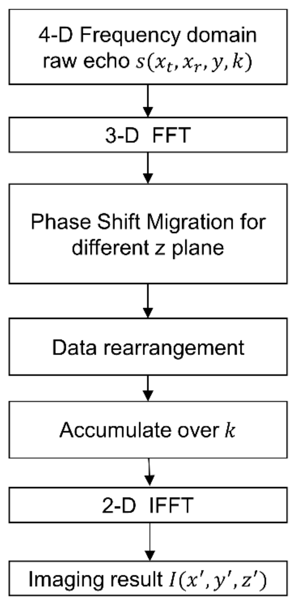
| Step 1. Conduct the 3D FT operation of the raw echo data to get the spatial wavenumber spectrum . Step 2. Apply the phase shift operator to migrate to the interest range plane , where is the discrete value of the distance of interest. Step 3. Perform the data rearrangement operation according to in the spatial wavenumber domain to convert the 5D data to 4D data . After data rearrangement, the bistatic MIMO data is converted to the monostatic imaging case. Step 4. Perform the spatial 2-D inverse FT of to obtained . Step 5. Sum over wavenumber k to form the final reconstructed image . |
| Output: 3-D MIMO-SAR imaging result |
| Input: Recorded raw echoes |
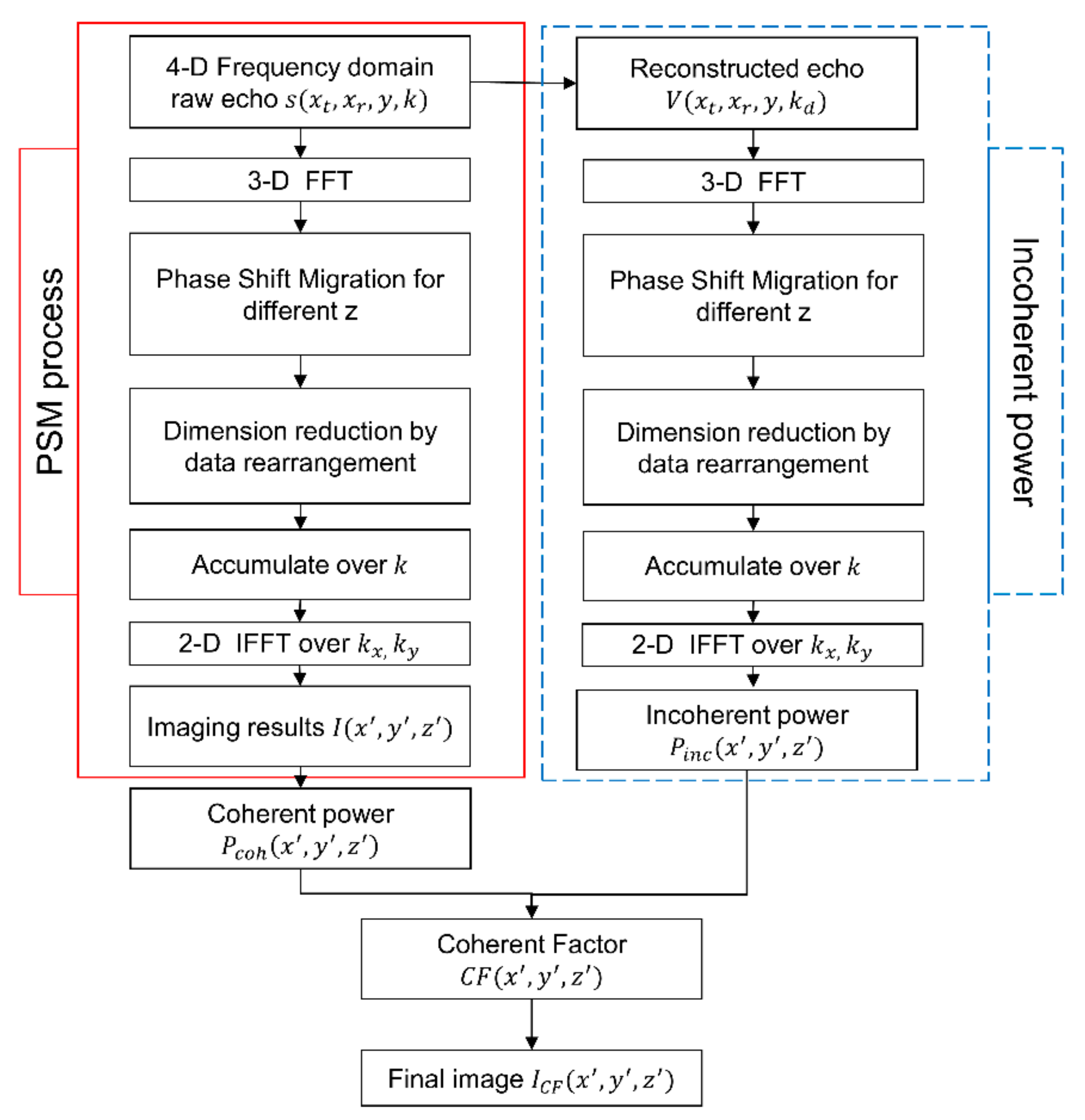
| Step 1. Calculate difference wavenumber according to , and reconstruct equivalent echo from raw echoes . Step 2. Perform the spatial 3-D FT operation of the recorded data and to obtain the wavenumber spectrum and . Step 3. Migrate and to the interest plane to get and by applying the phase-shift operator and . Step 4. Perform spatial frequency domain rearrangement according to to convert the 5-D data to 4-D and . After data rearrangement, the bistatic MIMO data are converted to the monostatic imaging case. Step 5. Perform the spatial 2-D inverse FT of and to obtained and . Step 6. Sum and over wavenumber k and to form the image and incoherent power . Step 7. Calculate the coherence factor coefficient according to (5). Step 8. Get the final image according to (7). |
| Output: 3-D MIMO-SAR imaging result after CF processing |
| Operation | FLOP |
|---|---|
| 3-D FFT | |
| Phase shift operation | |
| Data rearrange | |
| 2-D IFFT | |
| Sum along k | |
| Total |
| Parameters | Value |
|---|---|
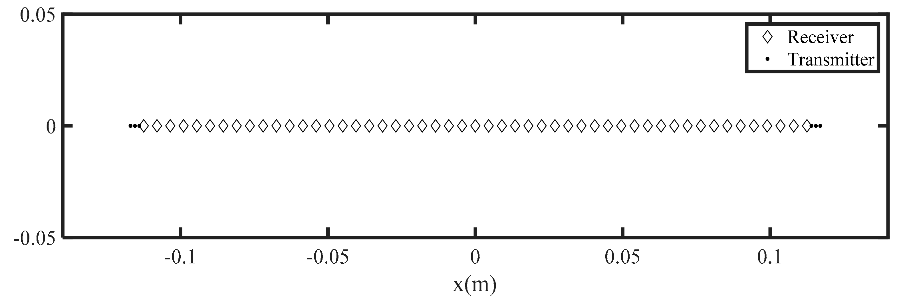
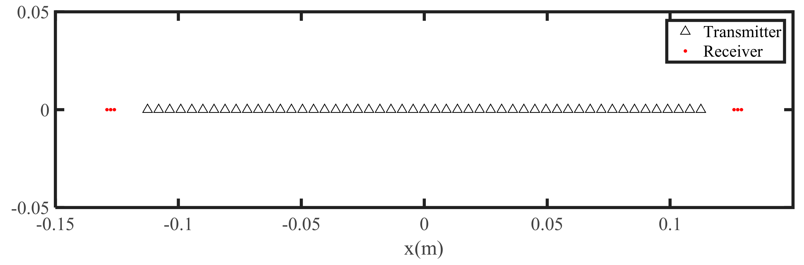
| The number of transmitters | 6 |
| The number of receivers | 51 |
| The interval of transmitters | 1.5 mm |
| The interval of receivers | 4.5 mm |
| Synthetic aperture scan interval | 2 mm |
| Center frequency | 0.3 THz |
| Bandwidth | 40 GHz |
| Frequency step | 200 MHz |
| Algorithms | FLOPs (1010) | Processing Time (s) |
|---|---|---|
| CF-BPA | 183.84 | 1976.57 |
| MCF-PSM algorithm | 1.75 | 7.83 |
Publisher’s Note: MDPI stays neutral with regard to jurisdictional claims in published maps and institutional affiliations. |
© 2021 by the authors. Licensee MDPI, Basel, Switzerland. This article is an open access article distributed under the terms and conditions of the Creative Commons Attribution (CC BY) license (https://creativecommons.org/licenses/by/4.0/).
Share and Cite
Yang, G.; Li, C.; Wu, S.; Zheng, S.; Liu, X.; Fang, G. Phase Shift Migration with Modified Coherent Factor Algorithm for MIMO-SAR 3D Imaging in THz Band. Remote Sens. 2021, 13, 4701. https://doi.org/10.3390/rs13224701
Yang G, Li C, Wu S, Zheng S, Liu X, Fang G. Phase Shift Migration with Modified Coherent Factor Algorithm for MIMO-SAR 3D Imaging in THz Band. Remote Sensing. 2021; 13(22):4701. https://doi.org/10.3390/rs13224701
Chicago/Turabian StyleYang, Guan, Chao Li, Shiyou Wu, Shen Zheng, Xiaojun Liu, and Guangyou Fang. 2021. "Phase Shift Migration with Modified Coherent Factor Algorithm for MIMO-SAR 3D Imaging in THz Band" Remote Sensing 13, no. 22: 4701. https://doi.org/10.3390/rs13224701
APA StyleYang, G., Li, C., Wu, S., Zheng, S., Liu, X., & Fang, G. (2021). Phase Shift Migration with Modified Coherent Factor Algorithm for MIMO-SAR 3D Imaging in THz Band. Remote Sensing, 13(22), 4701. https://doi.org/10.3390/rs13224701