Building Polygon Extraction from Aerial Images and Digital Surface Models with a Frame Field Learning Framework

Abstract

Deep learning-based models for building delineation from remotely sensed images face the challenge of producing precise and regular building outlines. This study investigates the combination of normalized digital surface models (nDSMs) with aerial images to optimize the extraction of building polygons using the frame field learning method. Results are evaluated at pixel, object, and polygon levels. In addition, an analysis is performed to assess the statistical deviations in the number of vertices of building polygons compared with the reference. The comparison of the number of vertices focuses on finding the output polygons that are the easiest to edit by human analysts in operational applications. It can serve as guidance to reduce the post-processing workload for obtaining high-accuracy building footprints. Experiments conducted in Enschede, the Netherlands, demonstrate that by introducing nDSM, the method could reduce the number of false positives and prevent missing the real buildings on the ground. The positional accuracy and shape similarity was improved, resulting in better-aligned building polygons. The method achieved a mean intersection over union (IoU) of 0.80 with the fused data (RGB + nDSM) against an IoU of 0.57 with the baseline (using RGB only) in the same area. A qualitative analysis of the results shows that the investigated model predicts more precise and regular polygons for large and complex structures.

1. Introduction

Buildings are an essential element of cities, and information about them is needed in multiple applications, such as urban planning, cadastral databases, risk and damage assessments of natural hazards, 3D city modeling, and environmental sciences [1]. Traditional building detection and extraction need human interpretation and manual annotation, which is highly labor-intensive and time-consuming, making the process expensive and inefficient [2]. The traditional machine learning classification methods are usually based on spectral, spatial, and other handcrafted features. The creation and selection of features depend highly on the experts’ knowledge of the area, which results in limited generalization ability [3]. In recent years, convolutional neural network (CNN)-based models have been proposed to extract spatial features from images and have demonstrated excellent pattern recognition capabilities, making it the new standard in the remote sensing community for semantic segmentation and classification tasks. As the most popular CNN type for semantic segmentation, fully convolutional networks (FCNs) have been widely used in building extraction [4]. An FCN-based Building Residual Refine Network (BRRNet) was proposed in [5], where the network comprises the prediction module and the residual refinement module. To include more context information, the atrous convolution is used in the prediction module. The authors in [6] modified the ResNet-101 encoder to generate multi-level features and used a new proposed spatial residual inception module in the decoder to capture and aggregate these features. The network can extract buildings of different sizes. In [7], Mask R-CNN is used to detect buildings by generating the bounding box of the individual building and producing precise segmentation masks for each of them. In [8], the authors adapted Mask R-CNN to building extraction and applied the Sobel edge detection algorithm to refine the uncompleted and poor edges. Although Mask R-CNN performed well in building instance segmentation, the authors in [6] found that the details of the building were lost when small feature maps were up-sampled to the same size of the input. While most geographic information system (GIS) applications need building polygons for visualization and analysis, traditional pixel-based segmentation methods are not able to produce accurate and regular building outlines. This is mainly because the segmentation network loses most of the edge location geometric features in the downsampling, while the process of upsampling focuses on semantic rather than location information. The imbalance between building content and boundary label pixels also brings difficulties for the learning progress [3]. Thus, conventional deep segmentation methods cannot extract sharp corners, producing undesired artifacts which need expensive and complex post-processing procedures to refine the results [9]. The rasterized segmentation results still need further processing to obtain buildings in polygon format.

Recent deep learning frameworks have been designed to obtain more regularized building polygons that are ready for GIS applications. The authors in [10] proposed PolyMapper, an end-to-end deep learning architecture that automatically extracts building boundaries in a vector format. However, compared with Mask R-CNN [7], the method produces less accurate outlines for large buildings [10]. Moreover, it is difficult to train and is not able to extract buildings with holes. In [3], building instance segmentation was improved by upgrading the feature extractor and detection module, and the performance of recurrent networks was accelerated by introducing convolutional Gated Recurrent Units (conv-GRU). 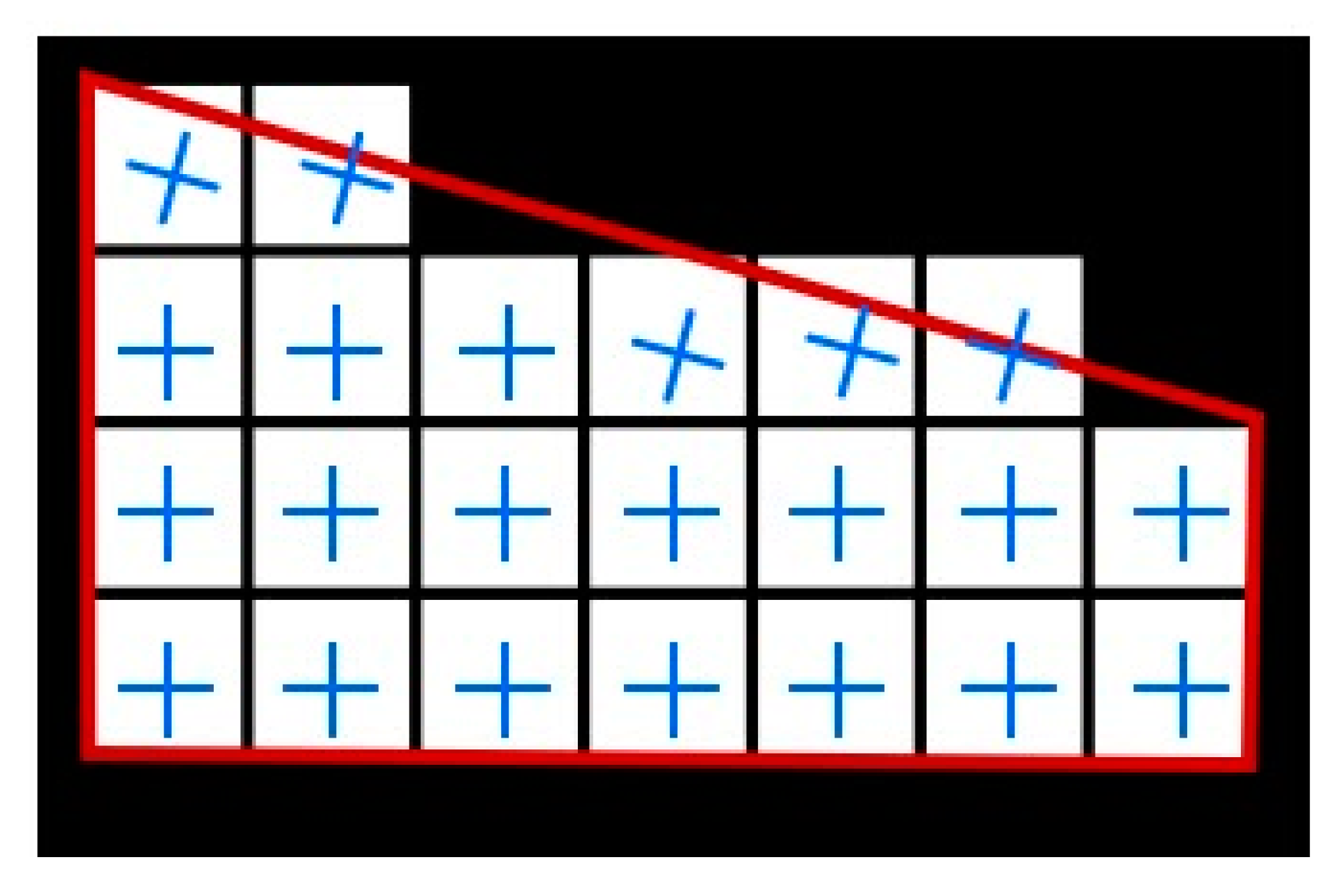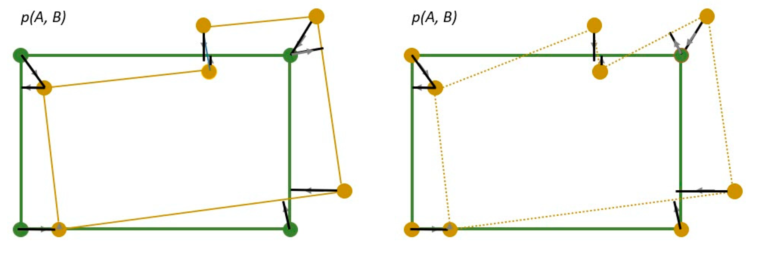Instead of using an end-to-end network with a complicated structure to directly produce polygons, in [9], a simpler FCN was trained to learn the building segmentation and the frame field. A frame field is comprised of two pairs of vectors with π symmetry each [11]. At least one field direction of the frame field is aligned with the tangent line of the contour when it locates along the building edges, as shown in Figure 1. Therefore, it stores the direction information of the tangent of the building outlines. With the additional frame field, the segmentation and polygon are improved. In this way, the method can produce regular and precise building outlines, especially for complex buildings with slanted walls that are usually a problem to most approaches.

Despite the recent progress made in this research field, accurately extracting buildings from optical images is still challenging due to the following reasons: (i) buildings have different sizes and spectral responses across the bands; (ii) trees or shadows often obscure them; and (iii) the high intra-class and low inter-class variations of building objects in high-resolution remote sensing images make it complex to extract the spectral and geometrical features of buildings [12]. Therefore, many methods of fusing other data sources have been proposed to solve such problems [13,14,15,16]. For instance, LiDAR sensors can penetrate through the sparse vegetation, and because of that, the elevation models derived from the LiDAR point cloud significantly alleviate the performance degradation caused by the limitations of optical images [13]. Similarly, digital surface models (DSMs) and nDSMs are popular options to provide 3D information in data fusion. A Fused-FCN4s network was proposed and tested on the combination of RGB, nDSM, and the panchromatic (PAN) band [15]. A Hybrid-PS-U-Net, which takes the low-resolution multispectral images and DSM as inputs directly, can extract complex and tiny buildings more accurately than Fused-FCN4s [16].

State-of-the-art methods that delineate buildings only consider spectral information from RGB imagery [9,10]. Since nDSMs contain 3D information about the height of the buildings, fusing aerial images with an nDSM has the potential to help overcoming aerial images’ limitations. We introduce nDSM and RGB data fusion to the framework to improve building outline accuracy. In this research, we aim to use a deep learning method to achieve end-to-end predictions of regularized vector outlines of buildings. Based on the existing frame field framework, we aim at improving the extraction performance by exploring the fusion of multi-source remote sensing data. In addition, we want to evaluate the vector outline extraction from different perspectives with new evaluation criteria. The three main contributions of this study are:

• We introduce the nDSM and near-infrared image into the deep learning model, using the fusion of images and 3D information to optimize information extraction in the building segmentation process.
• We evaluate the performance of the considered methods, adopting different metrics to assess the results at the pixel, object, and polygon levels. We analyze the deviations in the number of vertices per building extracted by the proposed methods compared with the reference polygons.
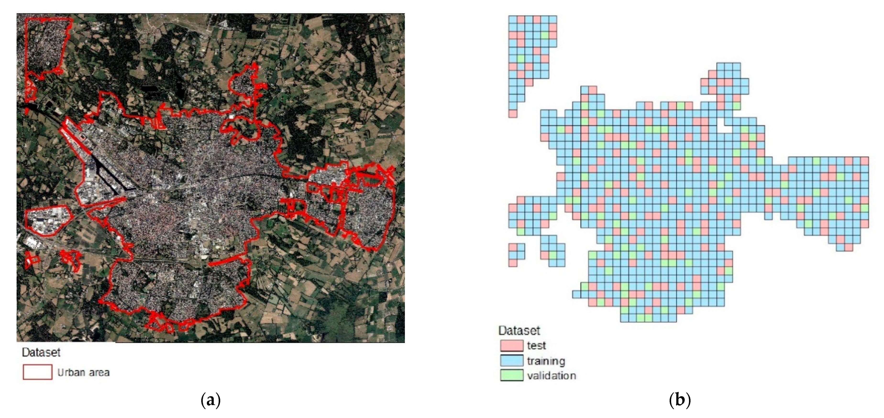
• We have constructed a new building dataset for the city of Enschede, The Netherlands, to promote further research in this field. The data will be published with the following DOI: 10.17026/dans-248-n3nd.

2. Proposed Method

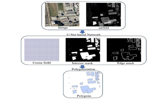
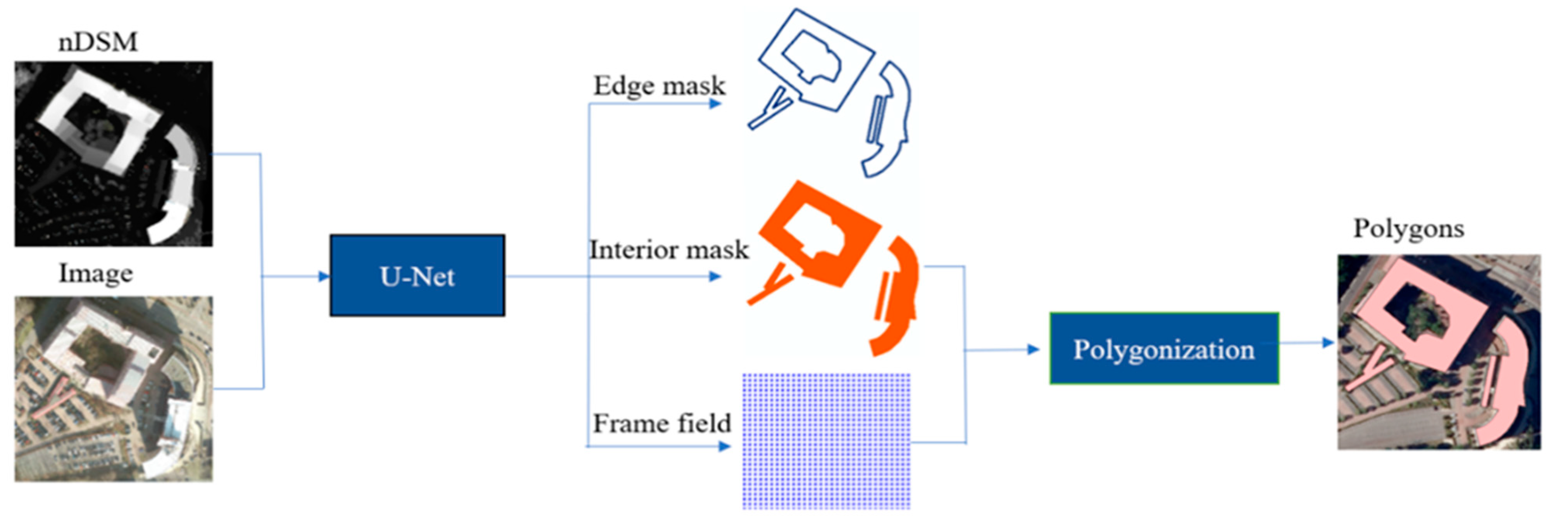
Our method is built upon [9] and is able to directly extract polygons from aerial images. We introduce the nDSM into the deep learning model to overcome the limitations of optical images, and the overall workflow is shown in Figure 2. At the first stage, a U-Net-like network [17] serves as a feature extractor to extract building segmentation and frame field, which are input into the following polygonization algorithm. The segmentation and frame field are improved by learning the additional information from the nDSM. Therefore, the data fusion helps to improve the final polygons.

At the second stage, the final polygons are generalized by multiple steps:

• First, an initial contour is produced from the segmentation;
• Then, the contour is iteratively adjusted with the constraints of the frame field;
• With the direction information of the frame field, the corners are identified from other vertices and further preserved in the simplification.

Two baselines were created for comparison to evaluate the performance gain due to the data fusion. One baseline takes as input the nDSM only; another one only analyzes the aerial images. To make it a fair comparison, all tiles of the different datasets were obtained with the same size and location; the network settings were also kept the same. By comparing the results obtained from data fusion with the two baselines, we can evaluate the improvements achieved, particularly the role of 3D information.

For the accuracy assessment, we evaluated our results at the pixel level, object level, and polygon level. Furthermore, we analyzed the deviations in the number of vertices per building extracted by the proposed methods compared with the reference polygons. This is an additional accuracy metric that captures the quality of the extracted polygons, a factor that is not considered in standard metrics. This allows us to estimate the additional complexity required for the editing operation, which is generally still required for operational applications (e.g., cadastral mapping or the generation of official national geographic datasets).

2.1. Frame Field Learning

A frame field is comprised of two pairs of vectors with π symmetry each [11]. “N-RoSy fields” are rotationally symmetric fields, which are special vector sets comprised of N unit-length vectors related by a rotation of an integer multiple of 2$\pi$/N. The N-PolyVectors are unordered vector sets in which no vector is necessarily related by any symmetry or magnitude to another [18]. The frame field is a 4-PolyVector field comprised of two coupled 2-RoSy fields [18]. The N-RoSy is the root set of the polynomials of the form $z^n-u^n$ [18]. If we denote the two coupled 2-RoSy fields as $u,v$ and the frame field as a ($u,v$) pair where $u,v\in C$, it then has an order-invariant representative, which is the pair representing the coefficients $C_0,C_2$ of the polynomial function in Equation (1) [9].

$$\left(z\right)=\left(z^2-u^2\right)\left(z^2-v^2\right)=z^4+c_2{z}^2+c_0$$

(1)

where $C_0,C_2\in C$. The frame field is the key element in this method. One direction is aligned to the tangent direction of the polygon when it is located along the building edges; if it is a corner, two directions should be aligned with the two edges comprising the corner. Therefore, it stores the direction information of the tangent of the building outlines. Instead of learning a ($u,v$) pair, a $\left(C_0,C_2\right)$ pair is learned per pixel because it has no sign or ordering ambiguity.

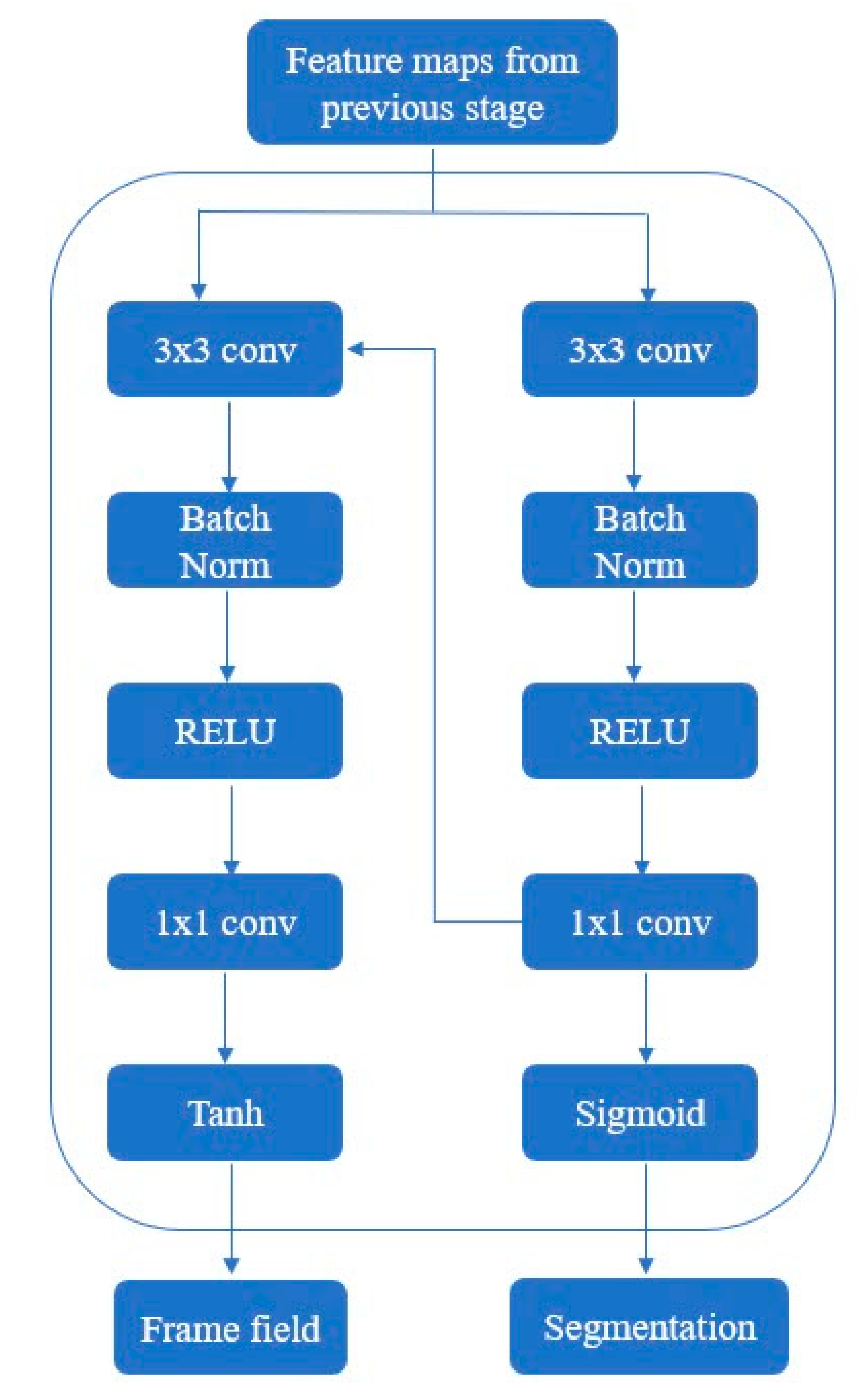
A multitask learning model is designed to learn the frame fields and segmentation masks of buildings. These related tasks help the model to focus on the important and representative features of the input data. The backbone of the model is a U-Net with 16 starting hidden features called U-Net16 [9]. The input layer of the backbone is extended to support taking input images with four or five channels. Then, the output features of the backbone are fed into two branches with a shallow structure. The specific structure is shown in Figure 3. The edge mask and interior mask are produced by one branch as two channels of a synthetic image. The frame field is produced by another branch that takes the concatenation of the segmentation output and the output features of the backbone as input and outputs an image of four channels.

The model is trained in a supervised way. In the pre-processing part of the algorithm, the reference polygons are rasterized to generate reference edge masks and interior masks. For a frame field, the reference is an angle of the tangent vector calculated from an edge of a reference polygon. Then, the angle is normalized to a range of (0,255) and stored as the value of the pixel where the edge of the reference polygon locates. For other pixels where there is no edge, the value is zero. The reference data for the frame field consist of an image with the same extent as the original input image.

2.2. Polygonization

The polygonization algorithm is composed of several steps. It takes the interior map and frame field of the neural network as inputs and outputs polygons corresponding to the buildings. First, an initial contour is extracted from the interior map by the marching squares algorithm [19]. Second, the initial contour is optimized by an active contour model (ACM) [20] to make the edges better aligned to the frame field. Third, a simplification procedure is applied to the polygons to produce a more regular shape. Finally, polygons are generated from the collection of polylines from the simplification, and the polygons with low probabilities are removed.

ACM is a framework used for delineating an object outline from an image [20]. The initial contour is produced by the marching square method from the interior map. The frame field and the interior map reflect different aspects of the building. The energy function is designed to constrain the snakes to stay close to the initial contour and aligned with the direction information stored in the frame field. Iteratively minimizing the energy function forces the initial contour to adjust its shape until it reaches the lowest energy.

The simplification is composed of two steps. First, the corners are found with the direction information of the frame field. Each vertex of the contour corresponds to a frame field comprised of two 2-RoSy fields and two connected edges. If two edges are aligned with different 2-RoSy fields, the vertex is considered a corner. Then, the contour is split at corners into polylines. The Douglas–Peucker algorithm further simplifies the polylines to produce a more regular shape. All vertices of the new polylines are within the tolerance distance of the original polylines. Hence, the hyperparameter tolerance could be used to control the complexity of the polygons.

2.3. Loss Function

The total loss function combines multiple loss functions for the different learning tasks: (1) segmentation, (2) frame field, and (3) coupling losses. Different loss functions are applied to the segmentation. Besides combining binary cross-entropy loss (BCE) and Dice loss (Dice), Tversky loss was also tested for edge mask and interior mask. Tversky loss was proposed to mitigate the issue of data imbalance and achieve a better trade-off between precision and recall [21]. The BCE is given by Equation (2).

$$L_{BCE}\left(\widehat{y},y\right)=\frac{1}{HW}{\displaystyle \sum }_{x\in I}\widehat{y}\left(x\right)·\log \left(y\left(x\right)\right)+\left(1-\widehat{y}\left(x\right)\right)·\log \left(1-y\left(x\right)\right)$$

(2)

where $L_{BCE}$ is the cross-entropy loss applied to the interior and the edge outputs of the model. H and W are the height and width of the input image, respectively. $\widehat{y}$ is the ground truth that is either 0 or 1. $y$ is the predicted probability for the class.

The Dice loss is given by Equation (3).

$$L_{Dice}\left(\widehat{y},y\right)=1-2·\frac{\left|\widehat{y}·y\right|+1}{\left|\widehat{y}+y\right|+1}$$

(3)

$$L_{int}=a·L_{BCE}\left({\widehat{y}}_{int},y_{int}\right)+\left(1-a\right)·L_{Dice}\left({\widehat{y}}_{int},y_{int}\right)$$

(4)

$$L_{edge}=a·L_{BCE}\left({\widehat{y}}_{edge},y_{edge}\right)+\left(1-a\right)·L_{Dice}\left({\widehat{y}}_{edge},y_{edge}\right)$$

(5)

where $L_{Dice}$ is the Dice loss, combined with the cross-entropy loss applied to the interior and the edge output of the model ($L_{int}$ and $L_{edge}$), respectively shown in Equations (4) and (5). $a$ is the hyperparameter, which was set to 0.25. $\widehat{y}$ is the ground truth label that is either 0 or 1. y is the predicted probability for the class.

The Tversky loss is given by the Equations (6) and (7).

$$T\left(\alpha ,\beta \right)=\frac{{{\displaystyle \sum }}_{i=1}^N{p}_{0i}{g}_{0i}}{{{\displaystyle \sum }}_{i=1}^N{p}_{0i}{g}_{0i}+\alpha {{\displaystyle \sum }}_{i=1}^N{p}_{0i}{g}_{1i}+\beta {{\displaystyle \sum }}_{i=1}^N{p}_{1i}{g}_{0i}}$$

(6)

$$L_{Tversky}=1-T\left(\alpha ,\beta \right)$$

(7)

where $p_{0i}$ is the probability of pixel $i$ being a building (edge or interior). $p_{1i}$ is the probability of pixel $i$ being a non-building. $g_{0i}$ is the ground truth training label that is 1 for a building pixel and 0 for a non-building pixel, and vice versa for the $g_{1i}$. The hyperparameter $\alpha$ was set to 0.15, and $\beta$ to 0.85.

A vector in a two-dimensional tangent space can be represented using Cartesian coordinates or equivalently as complex numbers. It is related to the angle-based representation via trigonometric functions or the complex exponential in Equation (8) [11].

$$\nu =\left(\begin{array}{c}\cos \left(\varphi \right)\\ \sin \left(\varphi \right)\end{array}\right)=e^{i\varphi }$$

(8)

The output frame field contains four channels, two each for the two complex coefficients $C_0,C_2\in C$ They define an equivalence class corresponding to a frame field. The reference is an angle ${\theta }_{\tau }\in \left[0,\pi \right)$ of the tangent vector of the building contour. The following losses are used to train the frame field.

$$L_{align}=\frac{1}{HW}{\displaystyle \sum }_{x\in I}{\widehat{y}}_{edge}\left(x\right)f{\left(e^{i{\theta }_{\tau }};C_0\left(x\right),C_2\left(x\right)\right)}^2$$

(9)

$$L_{align90}=\frac{1}{HW}{\displaystyle \sum }_{x\in I}{\widehat{y}}_{edge}\left(x\right)f{\left(e^{i{\theta }_{\tau }\perp };C_0\left(x\right),C_2\left(x\right)\right)}^2$$

(10)

$$L_{smooth}=\frac{1}{HW}{\displaystyle \sum }_{x\in I}(\Vert \nabla C_0\left(x\right){\Vert }^2+\Vert \nabla C_2\left(x\right){\Vert }^2)$$

(11)

From Equation (8), we know that $e^{i\varphi }$ is a vector tangent. In Equations (9) and (10), $e^{i{\theta }_{\tau }}$ represents a vector tangent to the building contour. ${\theta }_{\tau }$ is the direction of vector $\tau$, and ${\tau }^{\perp }=\tau -\frac{\pi }{2}$. $L_{align}$ makes the frame field more aligned with the tangent of the line segment of a polygon. $L_{align}$ is small when the polynomial $f\left(·;C_0,C_2\right)$ has a root near $e^{i{\theta }_{\tau }}$, meaning that one field direction is aligned with the direction of tangent $\tau$. $L_{align90}$ prevents the frame field from collapsing into a line field. $L_{smooth}$ produces a smooth frame field. Because these outputs are closely related and represent different information of the building footprints, the following functions, depicted in Equations (12)–(14), make them compatible with each other.

$$L_{int align}=\frac{1}{HW}{\displaystyle \sum }_{x\in I}f{\left(\nabla y_{int}\left(x\right);C_0\left(x\right),C_2\left(x\right)\right)}^2$$

(12)

$$L_{edge align}=\frac{1}{HW}{\displaystyle \sum }_{x\in I}f{\left(\nabla y_{edge}\left(x\right);C_0\left(x\right),C_2\left(x\right)\right)}^2$$

(13)

$$L_{int edge}=\frac{1}{HW}{\displaystyle \sum }_{x\in I}max\left(1-y_{int}\left(x\right),||\nabla y_{int}\left(x\right){||}_2\right)·|||\nabla y_{int}\left(x\right){||}_2-y_{edge}\left(x\right)|$$

(14)

where $L_{int align}$ and $L_{edge align}$ are used to force the interior mask $y_{int}$ and the edge mask $y_{edge}$ to be aligned with the frame field. $L_{int edge}$ makes the interior and edge masks compatible with each other.

3. Dataset

3.1. Dataset

The experiments were performed in Enschede, the Netherlands. The dataset contains three parts: (1) A VHR true ortho aerial image with 0.25 m spatial resolution provided by Kadaster [22]. It was acquired in the nationwide summer flight, and the acquired time was the year 2019. The Web Map Service (WMS) of the dataset is publicly available on PDOK [23]. The VHR image is composed of the bands red, green, blue, and near-infrared (NIR); (2) an nDSM that was obtained by subtracting the digital terrain model (DTM) from the DSM and then resampled to the same aerial image resolution. The DTM and DSM are publicly available on PDOK. The built-up area in DTM is “no-data”, which is filled by QGIS’ fill “nodata” tool with a maximum distance of 1000 pixels. AHN [24] is the digital elevation map for the Netherlands. The AHN3 dataset was acquired in the 3rd acquisition period (2014–2019) with a mean point density of 8-10 points/m². The dataset of the study area was acquired in 2019. The DTM and DSM were derived from point cloud data based on the squared IDW method with 0.5 m resolution. The LiDAR point clouds and DSM are shown in Figure 4. (3) Building footprints polygons were obtained from the publicly available geodata BAG [25] and used as training and reference data in our experimental analysis. The BAG is part of the government system of key registers captured by a municipality and subcontractors. There are some footprints that are not aligned with the ground truth, most of which are caused by human activities, such as buildings that are planned to be constructed but not yet started or buildings that are planned to be demolished and have been demolished. We edited them manually. Buildings with shared walls are difficult to distinguish for the network. The “dissolve” operation in QGIS was applied to BAG’s original polygons to merge them into one. The dissolve results are shown in Figure 5. Composite image 1 (RGB + nDSM) was produced by stacking the nDSM with the original aerial image as the 4th band. Composite image 2 (RGB + NIR + nDSM) was produced by stacking the NIR as the 4th band and nDSM as the 5th band with the original aerial image.

Our study area is composed of the urban area of Enschede. The extent and distribution of tiles are shown in Figure 6. Tiles are extracted from the aerial image (RGB), composite image 1 (RGB + nDSM), and composite image 2 (RGB + NIR + nDSM) with the same location and size. The dataset details are shown in

Table 1. The training set, validation set, and test set for the urban area using BAG reference polygons. The size of each tile is 1024 × 1024 pixels.

Dataset	Number of Tiles	Number of Buildings	Ratio
Training	579	29,194	0.7
Validation	82	4253	0.1
Test	165	8531	0.2

(the data will be released upon acceptance of the paper).

3.2. Evaluation Metrics

Pixel-level metrics. For evaluating the results, we used the IoU. IoU is computed by dividing the intersection area by the union area of a predicted segmentation (p) and a ground truth (g) at the pixel level.

$$IoU=\frac{area\left(p {\displaystyle \cap } g\right)}{area\left(p {\displaystyle \cup } g\right)}$$

(15)

Object-level metrics. Average precision (AP) and average recall (AR), defined in MS COCO measures, are introduced to evaluate our results. AP and AR are calculated based on multiple IoU values. IoU is the intersection of the predicted polygon with the ground truth polygon divided by the union of the two polygons. There are 10 IoU thresholds ranging from 0.50 to 0.95 with 0.05 steps. For each threshold, only the predicted results with IoU above the threshold will be count as true positives (tp). The rest will be denoted as false positives (fp). The ground truth with an IoU smaller than the threshold is a false negative (fn) [9]. Then, we use Equations (16) and (17) to calculate the corresponding precision and recall. AP and AR are the average values of all precisions and recalls, respectively, calculated over 10 IoU categories and can be denoted as mAP and mAR. AP and AR are also calculated based on the size of the objects: small (area < 32²), medium (32² < area < 96²), and large (area > 96²). The area is measured as the number of pixels in the segmentation mask. They can be denoted as AP_S, AP_M, and AP_L for the precision and AR_S, AR_M, and AR_L for the recall. We followed the same metric standards but applied them to building polygons directly. To be specific, the IoU calculation was performed based on polygons. For the alternative method, PolyMapper, as the data are in COCO format, the evaluation is based on segmentation in raster format.

$$P=\frac{tp}{tp+fp}$$

(16)

$$R=\frac{tp}{tp+fn}$$

(17)

with the average precision and average recall calculated based on COCO metrics standards. The F1 score—that is, the weighted average of precision and recall—can also be calculated by Equation (18).

$$F1=\frac{2·R·P}{R+P}$$

(18)

Polygon-level metrics. Besides the COCO metrics, polygons and line segments measurements (PoLiS) were introduced to evaluate the similarity of the predicted polygons to corresponding reference polygons. It accounts for positional and shape differences by considering polygons as a sequence of connected edges instead of only point sets [26]. We used this metric to evaluate the quality of the predicted polygon. We first filtered the polygons with IoU ≥ 0.5 to find the prediction polygons and the corresponding reference polygons. The metric is expressed as follows:

$$p\left(A,B\right)=\frac{1}{2q}{\displaystyle \sum }_{a_j\in A}\underset{b\in \partial B}{\min }||a_j-b||+\frac{1}{2r}{\displaystyle \sum }_{b_k\in B}\underset{a\in \partial A}{\min }||b_k-a||$$

(19)

where $p\left(A,B\right)$ is defined as the average of the distances between each vertex $a_j\in A$, j = 1, …, q, of A and its closest point $b\in \partial B$ on polygon B, plus the average of the distances between each vertex $b_k\in B$, k = 1, …, r, of B and its closest point $a\in \partial A$ on polygon A. The closest point is not necessarily a vertex; it can be a point on an edge. The variables (1/2q) and (1/2r) are normalization factors to quantify the overall average dissimilarity per point.

Figure 7 shows the PoLiS distance between A and B. A black line indicates the distance from the vertices of a polygon to another polygon, and its arrow shows the direction. The distance between a vertex and polygon could be a distance from a vertex to another vertex or a point on the edge of another polygon. The dotted light brown lines demonstrate one alternative way to connect point set B into a polygon. Even though it has the same vertices as the polygon connected by solid brown lines, the distance from the upper right corner of polygon A to polygon B is different. The shortest distance now points to another edge of polygon B, demonstrating that polygon shape changes influence the distance calculation.

To analyze the correlation between the number of vertices in the predicted polygon and its reference, we introduce the average ratio of the number of vertices and the average difference of the number of vertices. We first filter the polygons with IoU ≥ 0.5 to find the prediction polygons and the corresponding reference polygons. The average ratio of the number of vertices is computed by dividing the number of vertices of the predicted ones by that of their reference and then calculating the average value for all polygons, as shown in Equation (20). The average difference of the number of vertices is calculated by subtracting the number of vertices of the predicted ones from their references’ and then calculating the average value for all polygons shown in Equation (21). Root mean square error (RMSE) is also calculated by using the number of vertices of predicted polygons and their reference ones for all polygons, as shown in Equation (22).

$$Average ratio=\frac{1}{n}{\displaystyle \sum }_{i=1}^n\frac{{\widehat{v}}_i}{v_i}$$

(20)

$$Average difference=\frac{1}{n}{\displaystyle \sum }_{i=1}^n\left({\widehat{v}}_i-v_i\right)$$

(21)

$$RMSE=\sqrt{\frac{1}{n}{\displaystyle \sum }_{i=1}^n{\left({\widehat{v}}_i-v_i\right)}^2}$$

(22)

where ${\widehat{v}}_i$ is the number of the vertices for the predicted polygon and $v_i$ is the number of the vertices for the corresponding reference polygon.

3.3. Implementation Details

The model was trained with the following settings: the Adam optimizer with a batch size b = 4 and an initial learning rate of 0.001. It applies exponential decay to the learning rate with a decay rate of 0.99. The max epoch was set to 200. The network was implemented using PyTorch 1.4. We set several values (0.125,1,3,5,7,9) for the tolerance parameter in the polygonization method.

4. Results

We compared results obtained on the test set of aerial images (RGB) and composite images 1 (RGB + nDSM) and 2 (RGB + NIR + nDSM). To ensure a fair comparison of the two models, the configuration remains unchanged except for the input data.

4.1. Quantitative Analysis

Table 2. Results for the urban area dataset. The mean IoU is calculated on the pixel level. Other metrics are calculated on the polygons with 1-pixel tolerance for polygonization.

Bands	Loss Function	Mean IoU	mAP	mAR	F1	APS	ARS	APM	ARM	APL	ARL
RGB, NIR, nDSM	BCE + Dice	0.805	0.425	0.499	0.447	0.262	0.200	0.591	0.609	0.543	0.478
	Tversky	0.814	0.430	0.413	0.412	0.218	0.244	0.457	0.507	0.502	0.376
RGB, nDSM	BCE + Dice	0.800	0.410	0.488	0.433	0.255	0.198	0.576	0.593	0.534	0.465
	Tversky	0.776	0.371	0.399	0.373	0.204	0.197	0.441	0.482	0.464	0.650
RGB	BCE + Dice	0.568	0.067	0.253	0.102	0.139	0.024	0.285	0.261	0.248	0.232
nDSM	BCE + Dice	0.767	0.313	0.436	0.347	0.197	0.129	0.532	0.553	0.525	0.420

shows the quantitative results obtained using composite image 1 (RGB + nDSM), the single aerial images (RGB), and nDSM. The mean IoU achieved on composite image 1 is higher than others, demonstrating that the method benefited from the data fusion and performed better on the fused data than the individual data sources. The mean IoU achieved in the composite image 1 (RGB + nDSM) test set was 80% against 57% achieved for the test set of the RGB image. The addition of the nDSM led to an improvement of 23% in the mean IoU. Compared with the results obtained only using nDSM, the mean IoU achieved on composite image 1 (RGB + nDSM) is 3% higher, which shows that the addition of spectral information only led to a slight improvement of the mean IoU. Hence, we deduced that nDSM contributes more than aerial images in the building extraction. Moreover, the results obtained with only nDSM achieved a comparable accuracy which is close to besting the results obtained using composite image 2 (RGB + NIR + nDSM).

The same trend could also be found from the mAP and mAR of composite image 1 and the two baselines. The mAP and mAR achieved on composite image 1 are considerably higher than those achieved in aerial images (RGB) only and slightly higher than those achieved in the nDSM. Hence, we conclude that height information contributes more than spectral information in the building extraction. The higher average precision shows that height information helps to reduce the number of false positives, and higher average recall shows it helps prevent missing the real buildings on the ground. Composite image 1 achieved higher precision and recall for all building sizes, demonstrating that it outperformed the individual source in all sizes of the buildings. In terms of size, buildings of medium size have the highest precision and recall. Small buildings have the lowest precision and recall, which means the model performs better for medium buildings and worse for small buildings. Fewer small buildings are correctly extracted, and more false positives are polygons of small size.

Comparing the results obtained from the two composite images, the mean IoUs obtained with the BCE and Dice loss were almost the same, but the average precision and recall achieved on composite image 2 (RGB + NIR + nDSM) were slightly higher. This means that the NIR information helps to reduce the number of false positives and prevent missing the real buildings on the ground. Tversky loss achieved the highest mean IoU (81.4%) and the highest average precision (43%) on composite image 2 (RGB + NIR + nDSM) among all the experiments. High precision means that among the prediction polygons, most of them correspond to real buildings on the ground. A high recall means that among the reference buildings, most of them are found and delineated correctly. The F1 score achieved in the same dataset with BCE and Dice loss is the highest. F1 conveys the balance between precision and recall. The higher F1 value means the BCE and Dice loss can predict buildings more correctly and avoid missing the real buildings. It achieved a better balance between precision and recall.

In terms of the similarity among the polygons,

Table 3. PoLiS results for the urban area dataset. The PoLiS are calculated on the polygons with 1-pixel tolerance for polygonization.

Bands	Loss	PoLiS
RGB, NIR, nDSM	BCE + Dice	0.52
	Tversky	0.62
RGB, nDSM	BCE + Dice	0.54
	Tversky	0.62
RGB	BCE + Dice	0.87
nDSM	BCE + Dice	0.62

shows that the PoLiS distance achieved on composite image 1 (RGB + nDSM) with the BCE and Dice loss is 0.54, considerably smaller than 0.87 for the RGB image and slightly smaller than 0.62 for the nDSM. The smaller PoLiS distance means less dissimilarity, showing that the data fusion achieved better similarity than individual data sources. The PoLiS distance obtained in the nDSM is smaller than that obtained in aerial images, which means the nDSM contributes more than aerial images in improving the similarity for results obtained from the composite images. The PoLiS distance achieved on composite image 2 (RGB + NIR + nDSM) with the BCE and Dice loss is 0.52, which is smaller than 0.54 achieved on composite image 1 (RGB + nDSM), demonstrating that the additional NIR information further improves the similarity. Furthermore, for the same composite images, the PoLiS distance of the model with the BCE and Dice loss is smaller than that with Tversky loss, which means the polygons produced by the combination of BCE and Dice loss are more similar to their reference.

4.2. Qualitative Analysis

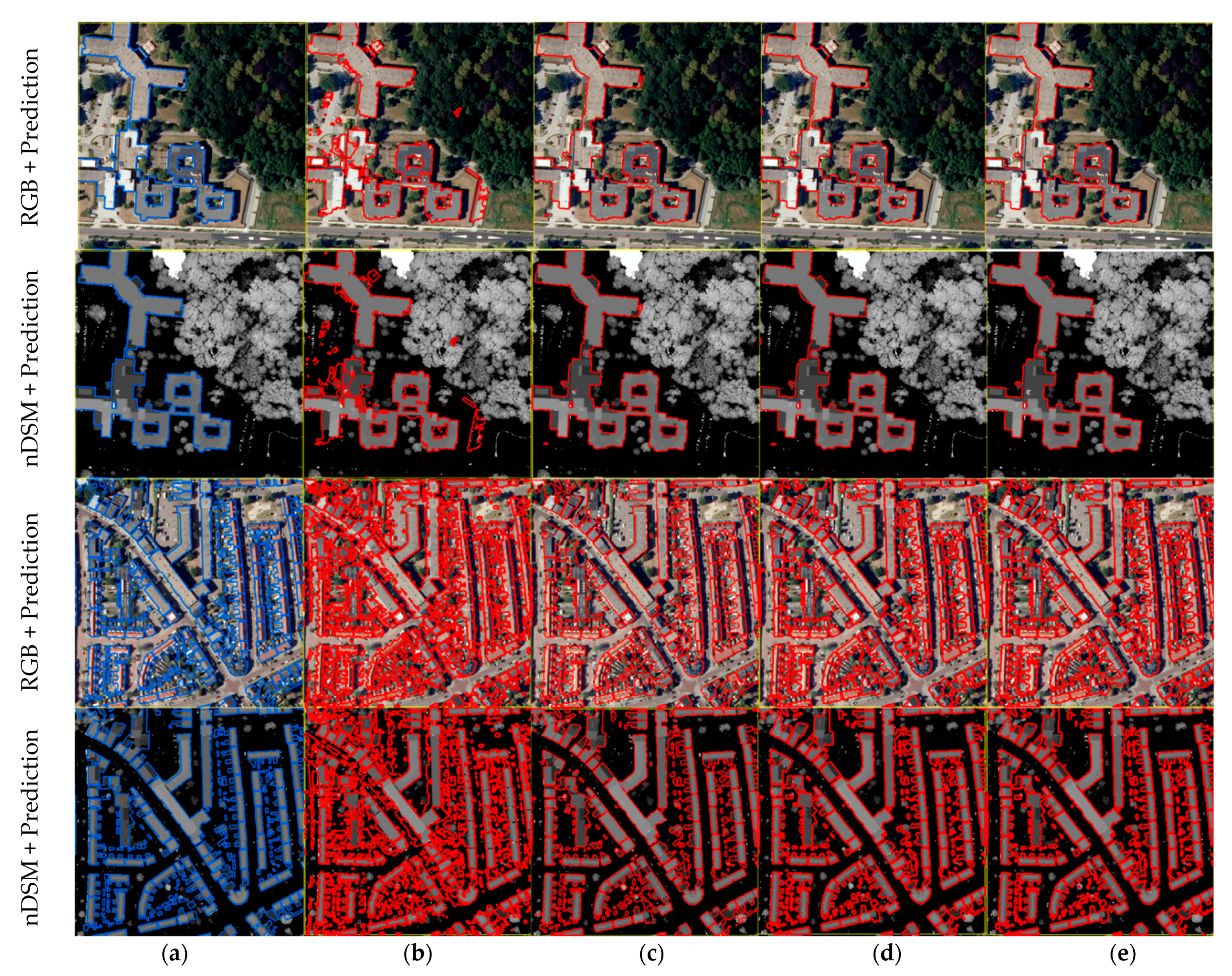
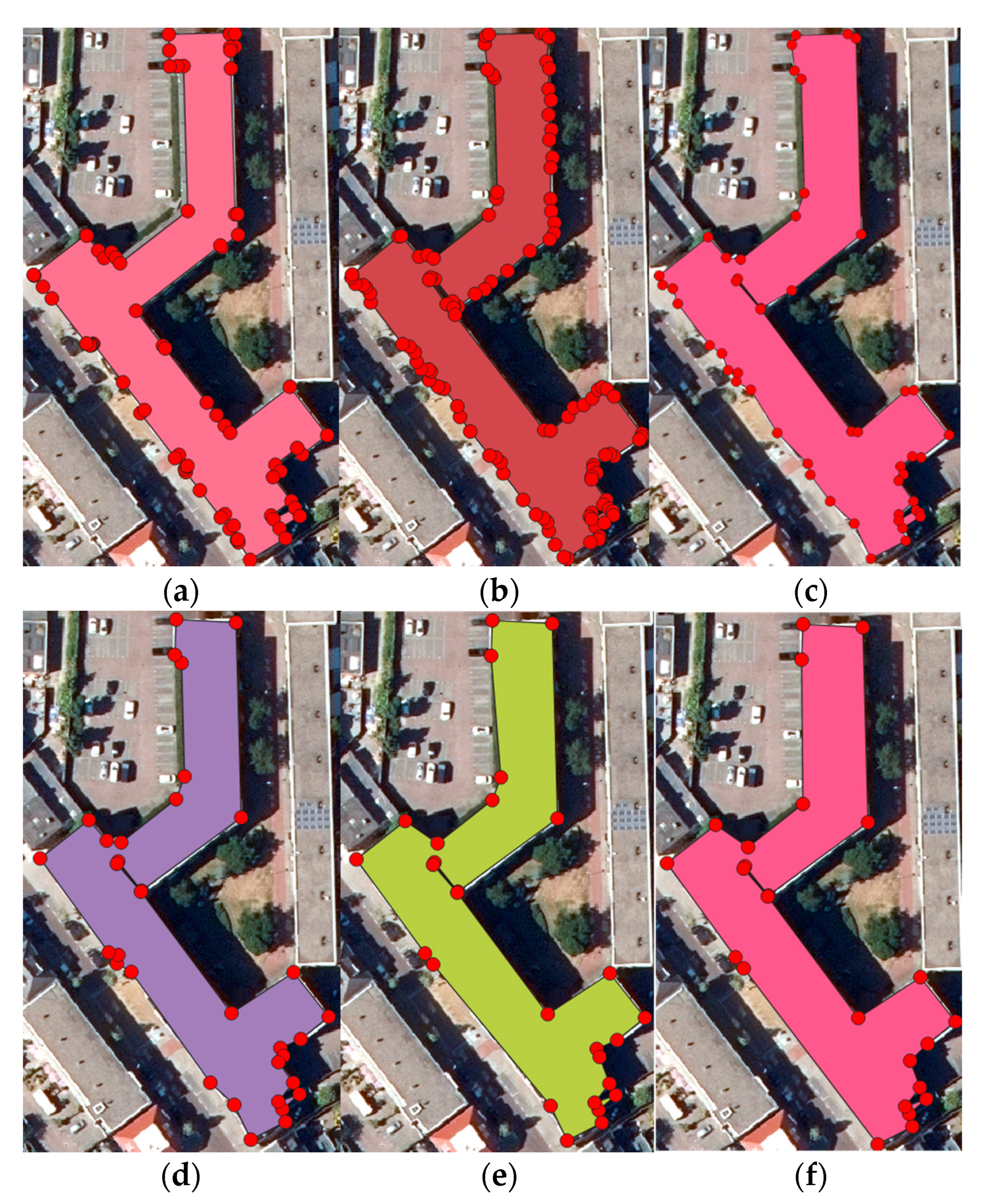
Figure 8 compares the predicted polygons obtained on tiles in the test set with different bands and the corresponding reference. The polygons obtained using the composite images are more aligned with the reference data and with fewer false positives than those obtained from RGB images or the nDSM only. The performance gain is particularly visible for big buildings with complex structures and buildings with holes. Fewer false positives are observed for small buildings in the results obtained using composite images. Compared with the polygons obtained from RGB images, the polygons obtained from the nDSM have fewer false positives and are more aligned with ground truth. In addition, the polygons of large buildings are more regular than the small ones in dense urban areas. There are more false positives for small buildings in dense urban areas than in sparse areas. By visual observation, we may conclude that some of them are storage sheds or garden houses, which are not included in the reference footprints. Their similar spectral character and height make it difficult to differentiate them from residential buildings. In summary, the nDSM improved building outlines’ accuracy, resulting in better-aligned building polygons and preventing false positives. The polygons obtained from different composite images are very similar to each other.

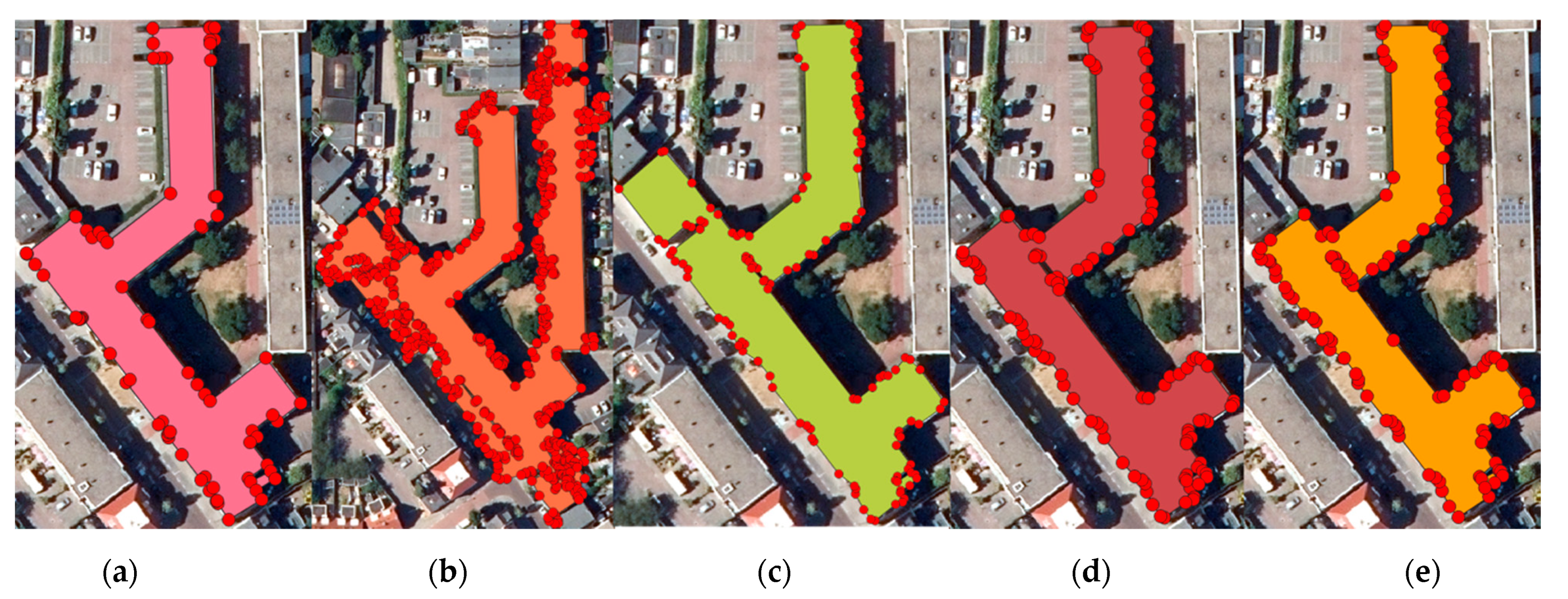
Figure 9 shows the predicted polygon on different datasets. Comparing the polygon obtained in the aerial image (RGB) with that on composite image 1 (RGB + nDSM) shows that the model cannot differentiate nearby buildings with only spectral information. This results in the predicted polygon in the aerial image (RGB) corresponding to several individual buildings. In addition, part of the road on the left side of the building is considered to be a building. Comparing the polygon obtained with the nDSM with that on composite image 1 (RGB + nDSM) shows that the model cannot differentiate closed buildings with only height information. This results in the upper right building being considered as part of the predicted building. Comparing the predicted polygons on composite image 1 (RGB + nDSM) with those on composite image 2 (RGB + NIR + nDSM) shows that the general shapes are very similar to each other, the numbers of the vertices are almost the same, but the distributions are different. During the simplification phase of the polygonization process, the corners are kept while the other vertices are further simplified. Hence, the corners are different as well. The additional NIR also affects the corner detection.

Table 4. Results for the urban area dataset. The mean IoU is calculated on the pixel level. Other metrics are calculated on the polygons with 1-pixel tolerance for polygonization. The polygons a, b, c, d, and e correspond to the polygons (a), (b), (c), (d), and (e) in Figure 9.

Polygon	Dataset	PoLiS	Vertices
a	reference		74
b	RGB	5.32	612
c	nDSM	0.81	44
d	RGB + nDSM	0.47	112
e	RGB + NIR + nDSM	0.39	111

shows the PoLiS distance of the example polygon. The polygon obtained on composite image 2 (RGB + NIR + nDSM) has the smallest distance, which is 0.39 against 0.47 for that of composite image 1 (RGB + nDSM). Hence, the additional NIR information helps to improve the similarity between the predicted polygon and the reference polygon. The PoLiS distance achieved with the nDSM is 0.81, which is considerably smaller than the 5.32 obtained from aerial images only, demonstrating that the nDSM increased the similarity significantly.

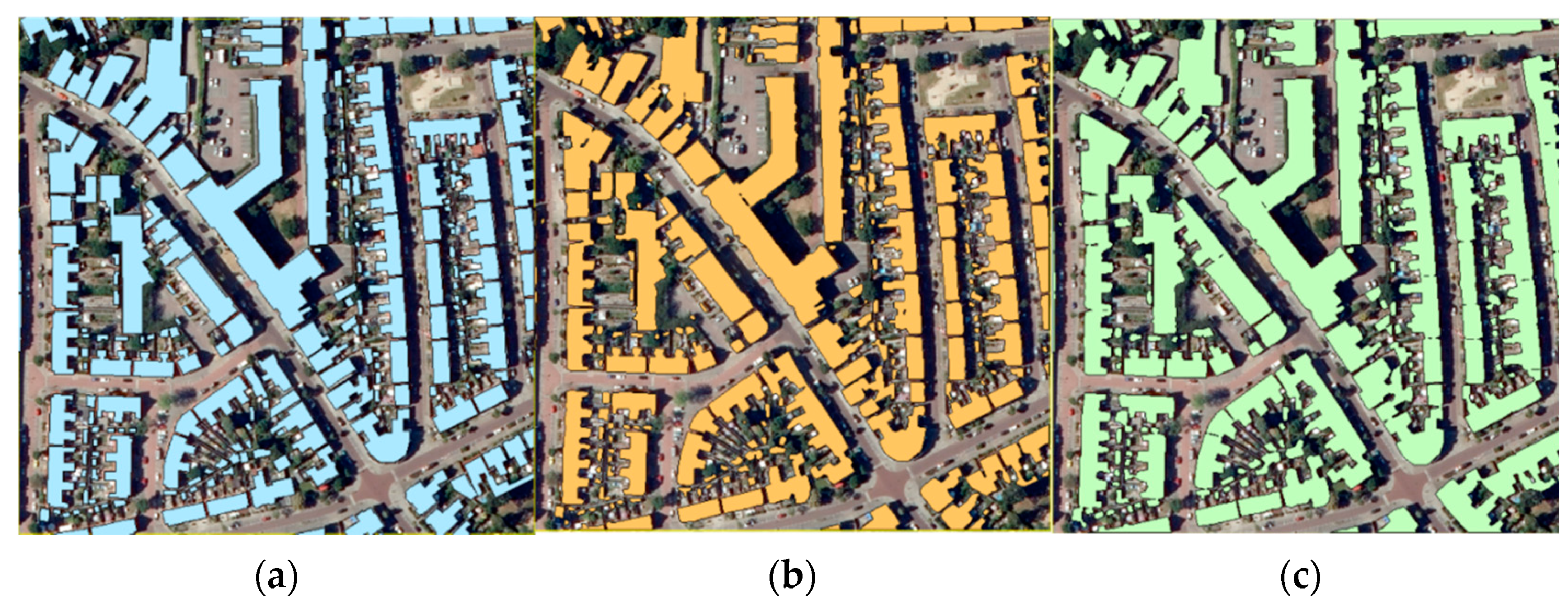
Figure 10 shows the predicted polygons obtained on composite image 2 (RGB + NIR + nDSM) with different losses. Compared with the reference polygons, the polygons obtained with the Tversky loss function are much bigger, which means that the non-building area close to the building is also being recognized as a building. Compared with polygons obtained with BCE and Dice loss, some buildings are connected to each other, which means that it is hard to separate buildings close to each other with Tversky loss. The same problems also appear in the results with different losses obtained on composite image 1 (RGB + nDSM). It could be deduced that the combination of BCE and Dice loss helps in producing polygons that are more aligned with ground truth.

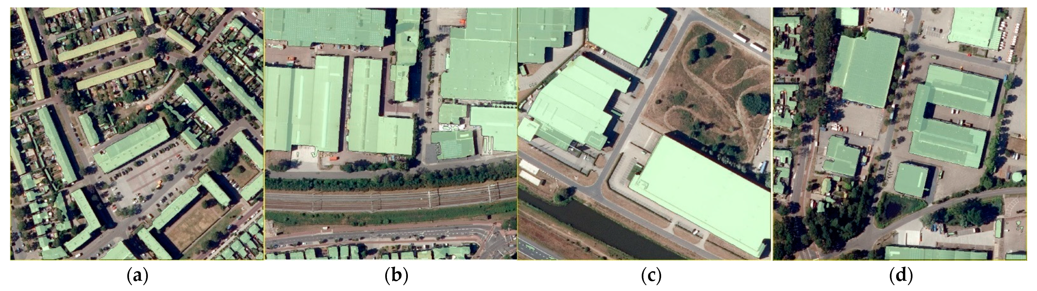
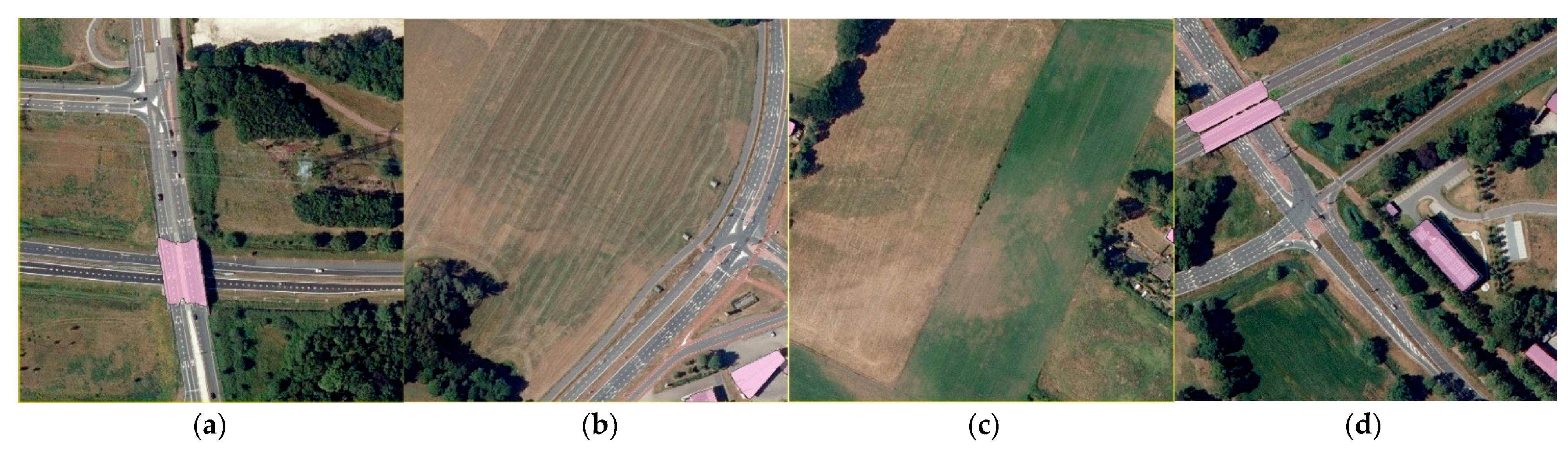
Figure 11 shows the predicted polygons obtained on composite image 1 (RGB + nDSM) with a high mean IoU. Besides the first one, buildings in other tiles are big and regular buildings, showing that our method performed well for big and regular buildings. Figure 12 shows the predicted polygons obtained on composite image 1 (RGB + nDSM) with a low mean IoU. These results show that our method performed worse for the sparse urban area with large green fields. There are two false positives on the overpass. 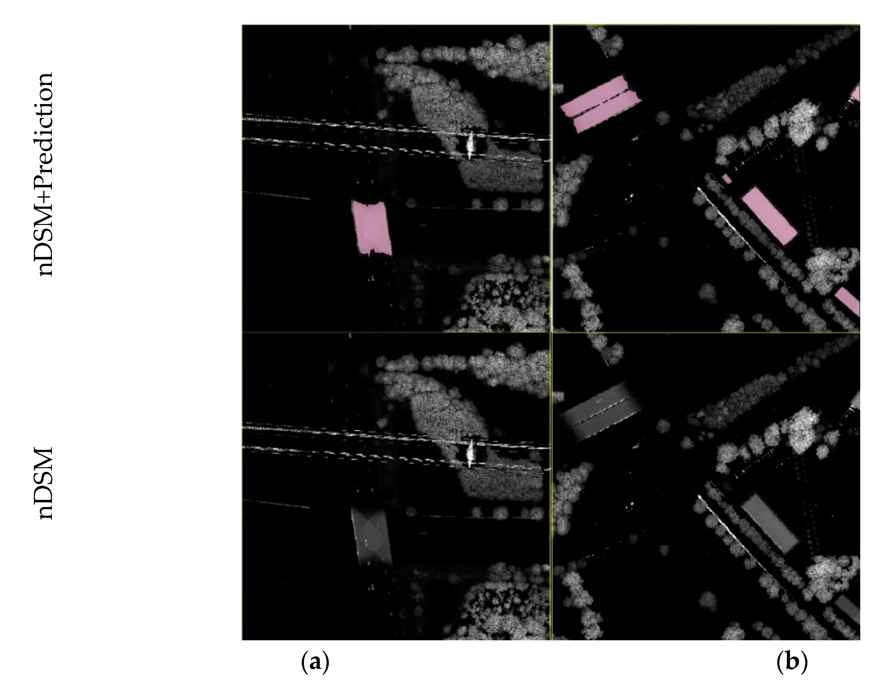Figure 13 shows the comparison of the two false positives with the nDSM; the height of the false positives on the overpass is higher than its surroundings. We may deduce that the nDSM results in the false positives for the overpass.

4.3. Analysis of the Number of Vertices

The last phase of the polygonization method is a simplification that produces more generalized polygons. The tolerance of the simplification is an important parameter to balance the complexity and fidelity of polygons. We perform an analysis of the number of vertices per polygon by changing the tolerance value. We first filter the polygons with IoU ≥ 0.5 to find the predicted polygons and the corresponding reference polygons. Besides the RMSE, we introduced the average ratio of vertices number and the average difference of vertices number to analyze the similarity of the vertices numbers. For the ratio, the best value is 1, which means the average vertices number is the same as its reference. The closer the ratio is to 1, the higher the similarity of the number of vertices. The best value for the difference is zero, which means the average vertices number of the predicted polygons is the same as its reference. The closer the difference value is to zero, the higher the similarity of the vertices numbers. The negative difference value means the average vertices number of predicted polygons is smaller than that of its reference.

Table 5. Polygon obtained with different tolerances using the composite image 1 (RGB + nDSM) for urban area dataset.

Tolerance	PoLiS	RMSE	Average Ratio of Vertices Number	Average Difference of Vertices Number
1	0.536	80.40	1.621	5.327
3	0.567	81.44	1.026	−3.588
5	0.588	83.07	0.935	−5.236
7	0.611	71.50	0.899	−5.426
9	0.636	72.96	0.872	−6.138

shows an analysis of the number of vertices of the results obtained on composite image 1 (RGB + nDSM) with BCE and Dice as the loss. Even though tolerance 1 has the smallest PoLiS, the ratio is the biggest among all the results. The PoLiS distance represents polygon dissimilarity, and a smaller distance means a higher similarity. The polygons obtained with tolerance 1 have the most similar shape to their reference but contain more vertices than the reference. The ratios of tolerance 3, 5, 7, and 9 are close to each other, but tolerance 3 results in the difference closest to zero and the ratio closest to one, demonstrating the number of predicted vertices most comparable to the reference. The distance increases as the tolerance increases, and tolerance 3 results in the second-smallest PoLiS value. Therefore, we may deduce that tolerance 3 results in generalized polygons that contain a similar number of vertices as the reference without losing too much positional and shape accuracy. Similar trends also exist in the results obtained on composite image 2 (RGB + NIR + nDSM). Therefore, we deduce that 3 is an appropriate tolerance to obtain the best-generalized polygons without losing too much similarity for our dataset.

Figure 14 compares the predicted polygon with different tolerance levels. For the sample building, the increase in tolerance results in the decrease in the number of vertices.

Table 6. Example polygon with different tolerances and numbers of vertices. The polygons a, b, c, d, e, and f correspond to the polygons (a), (b), (c), (d), (e), and (f) in Figure 14.

Polygon	Tolerance	PoLiS	Vertices	Ratio
a			74
b	1	0.472	112	1.514
c	3	0.537	52	0.703
d	5	0.628	35	0.473
e	7	0.697	29	0.392
f	9	0.763	26	0.351

shows that the PoLiS value increases as the tolerance increases, which means the dissimilarity of the predicted polygon and reference polygon is increasing. Compared to the polygon predicted with tolerance 1, changes happen to the shape of the polygons with bigger tolerance, such as the edge in the upper part of the polygons deviating from the ground truth.

For the predicted polygons with 1-pixel tolerance, even though it has a high positional accuracy, it contains the largest number of vertices. Furthermore, most vertices are so close to each other that some of them are superfluous. If manually simplifying the polygon, compared to the reference, a lot of vertices need to be removed, which increases the processing time and waste of human labor. For polygons predicted with the best tolerance found by the analysis of the number of vertices, the outlines have a similar shape but fewer vertices. Thus, fewer editing operations need to be performed to move or delete vertices, which may simplify the post-processing procedure.

4.4. Comparison with Alternative Methods

We compared the frame field learning-based method to the end-to-end polygon delineation method PolyMapper [10]. The experiments are performed on the original aerial images (RGB). The default setting of the PolyMapper method is adopted with the max iteration of 1,600,000, and the backbone is ResNet-101.

Table 7. Results obtained using aerial images (RGB) for the urban area dataset. The metrics are calculated on the polygons with 1-pixel tolerance for polygonization for the frame field learning-based method.

Method	mAP	mAR	APS	ARS	APM	ARM	APL	ARL
PolyMapper	0.009	0.017	0.001	0.001	0.004	0.028	0.014	0.065
Frame field	0.067	0.253	0.139	0.024	0.285	0.261	0.248	0.232

shows a quantitative comparison of two methods reported in COCO metrics. The frame field learning-based method achieves 6.7% mAP and 25.3% mAR, outperforming PolyMapper significantly. The results demonstrate that the frame field approach correctly extracts a higher proportion of buildings. In addition, the method works significantly better in delineating medium and large buildings and achieves higher precision at all scale levels.

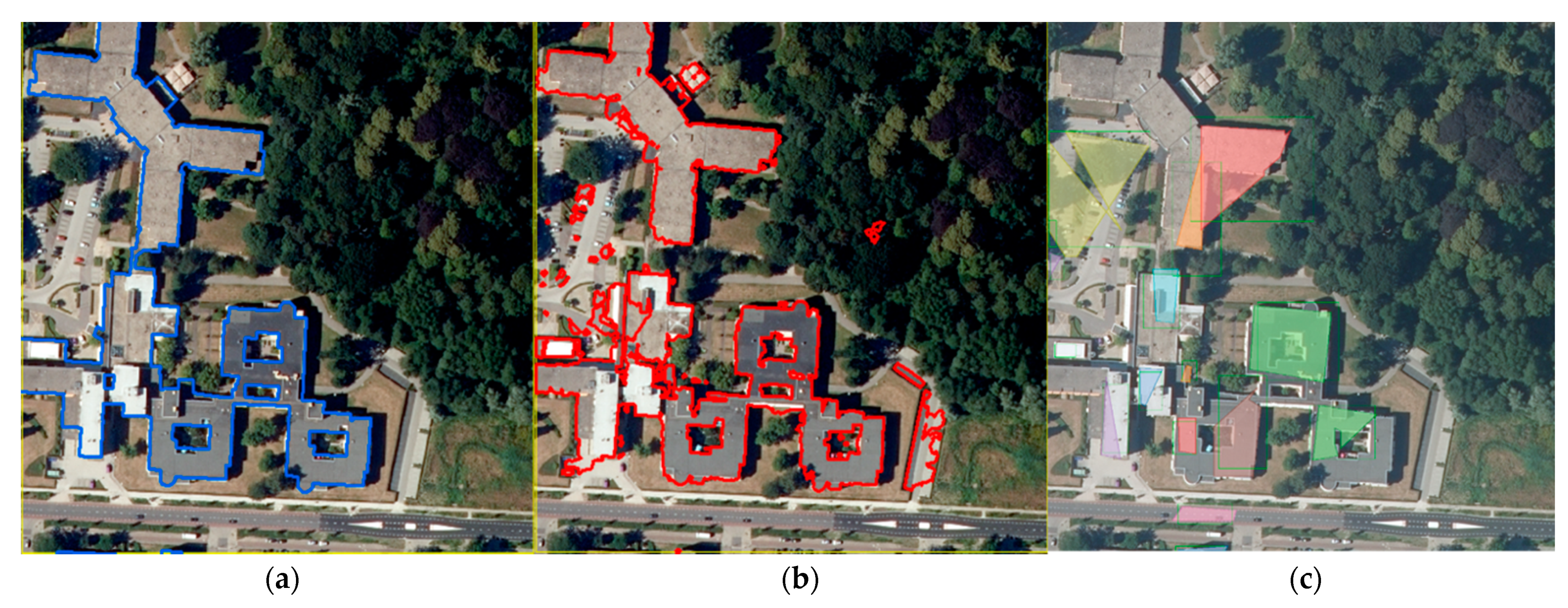
Figure 15 shows the results obtained on two tiles by different methods. PolyMapper only extracts part of the large buildings, and it cannot delineate the hole inside the building. It cannot differentiate individual buildings from the surrounding road and trees, and it misses large parts of real buildings on the ground. The frame field learning method extracted more buildings with more regular and aligned predicted polygons. However, many false positives exist in the results obtained by the frame field method compared with the reference data. Some individual buildings in the densely urban areas are also connected, demonstrating that it cannot differentiate buildings that are close to each other with only the spectral information.

4.5. Limitations and Insights

There are some limitations to the proposed method. This study shows that the nDSM has improved accuracy by a large margin due to the additional height information provided. Besides, high-resolution nDSMs and 3D information contribute more than spectral information. In the Netherlands, nDSM data are openly available. However, high-resolution elevation data are unfortunately not openly available in most countries. This may limit the applicability of the proposed method to areas where elevation data are available. LiDAR data are usually associated with expensive acquisition campaigns. A cheaper solution could be extracting a DSM and point clouds via dense matching techniques from stereo aerial images. Where this option is also not possible, solutions based on monocular depth estimation using generative adversarial networks could be explored [27,28].

An additional problem is that the DSM and the aerial image must be collected at nearby times, making this method hard to implement. The results largely rely on the quality of each individual data source and the degree to which they are consistent with each other. The buildings in each individual dataset should be aligned with each other. To avoid the changes that happen in the time gap that cause discrepancy, the acquisition times of the data should be as close as possible. The BAG dataset is produced by municipalities and subcontractors, and data qualities may vary from one city to another. The conclusions obtained for Enschede are therefore not necessarily applicable to BAG data from another region.

5. Conclusions

In this study, we explored a building delineation method based on frame field learning. The overall framework of our method is based on an FCN architecture, which serves as an extractor of image segmentation and direction information of the building contour, followed by a polygonization method, which takes the outputs of the model as inputs to generate the polygons in a vector format.

Our method combines the deep learning framework with data fusion by taking two different composite images (RGB and nDSM; RGB, NIR, and nDSM) as input. Compared with the results obtained in the two baselines (RGB only and nDSM only), the polygons obtained on composite images were largely improved, considering both quantitative and qualitative criteria. The method benefited from the additional nDSM, and the height information contributed more than spectral information in building extraction.

We introduced new evaluation criteria which assessed the results at the pixel, object, and polygon levels. We also performed an analysis of the number of vertices and introduced the average ratio of the number of vertices and the average difference of the number of vertices to evaluate the agreement between the predicted polygon and its reference. This evaluation criterion provides relevant information about the quality of the extracted polygons for practical application. For example, by analyzing these two statistical metrics in combination with PoLiS distance for the polygons produced with different tolerances, we found the best parameters for our model to produce simpler polygons while keeping high accuracy. For applications that require high accuracy (e.g., cadastral mapping), the predicted polygons need additional post-processing steps to validate the quality of the data and correct errors. The predicted polygons with fewer vertices and comparable accuracy will facilitate this process and reduce the manual work.

Our approach can help cartographic institutions such as the cadaster to generate and update building footprints more effectively. Furthermore, the building polygons can also be used in other products, such as topographic maps and building models. Our further study will focus mainly on the following research lines: (1) explore different fusion strategies, (2) refine the training strategy, (3) explore and compare the proposed method against other polygonization methods, and (4) test the generalization and transferability of the model to other regions.