
A Machine Learning Based Downscaling Approach to Produce High Spatio-Temporal Resolution Land Surface Temperature of the Antarctic Dry Valleys from MODIS Data


Abstract
:1. Introduction
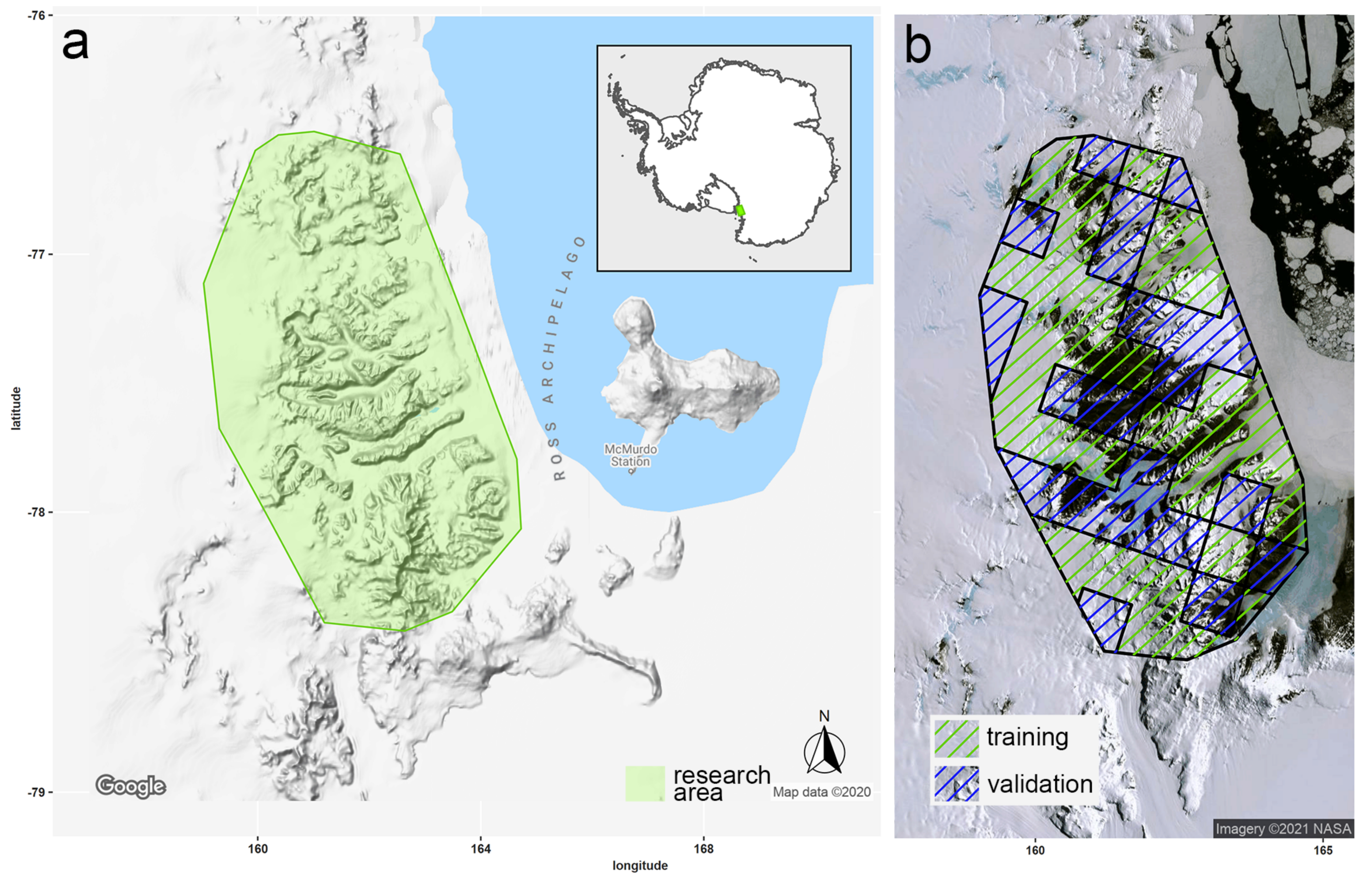
2. Research Area
3. Material and Methods
3.1. Data and Pre-Processing
3.1.1. Landsat LST
3.1.2. MODIS LST
3.1.3. High Resolution Predictors for LST
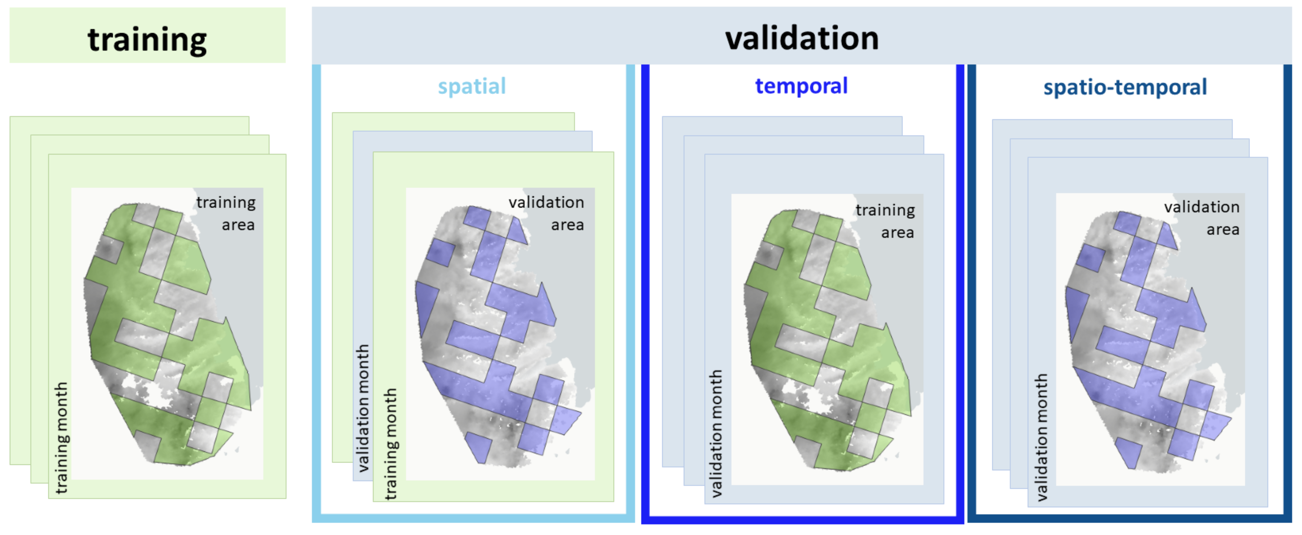
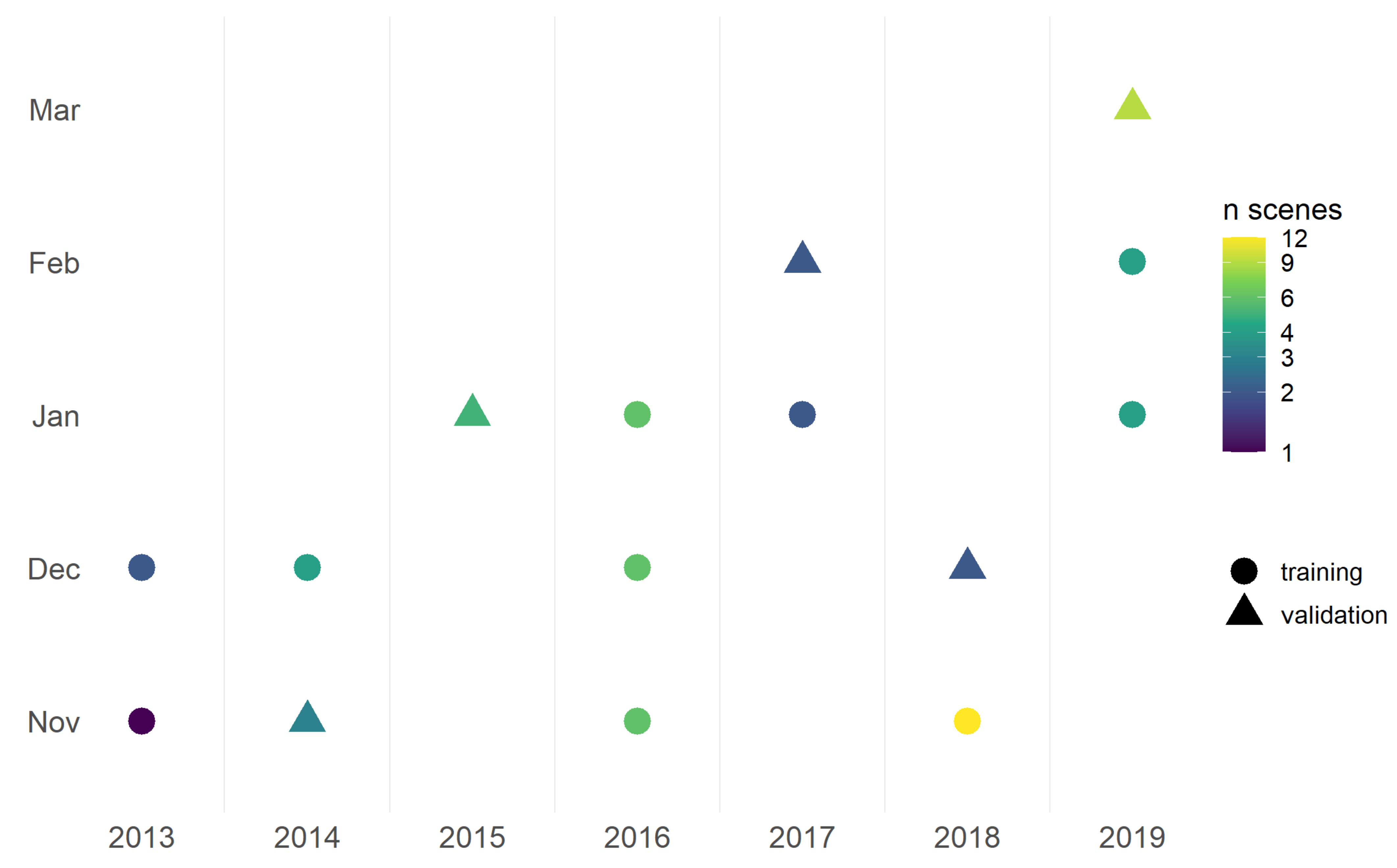
3.2. Compilation of the Training and Validation Data Sets
3.3. Training and Validation
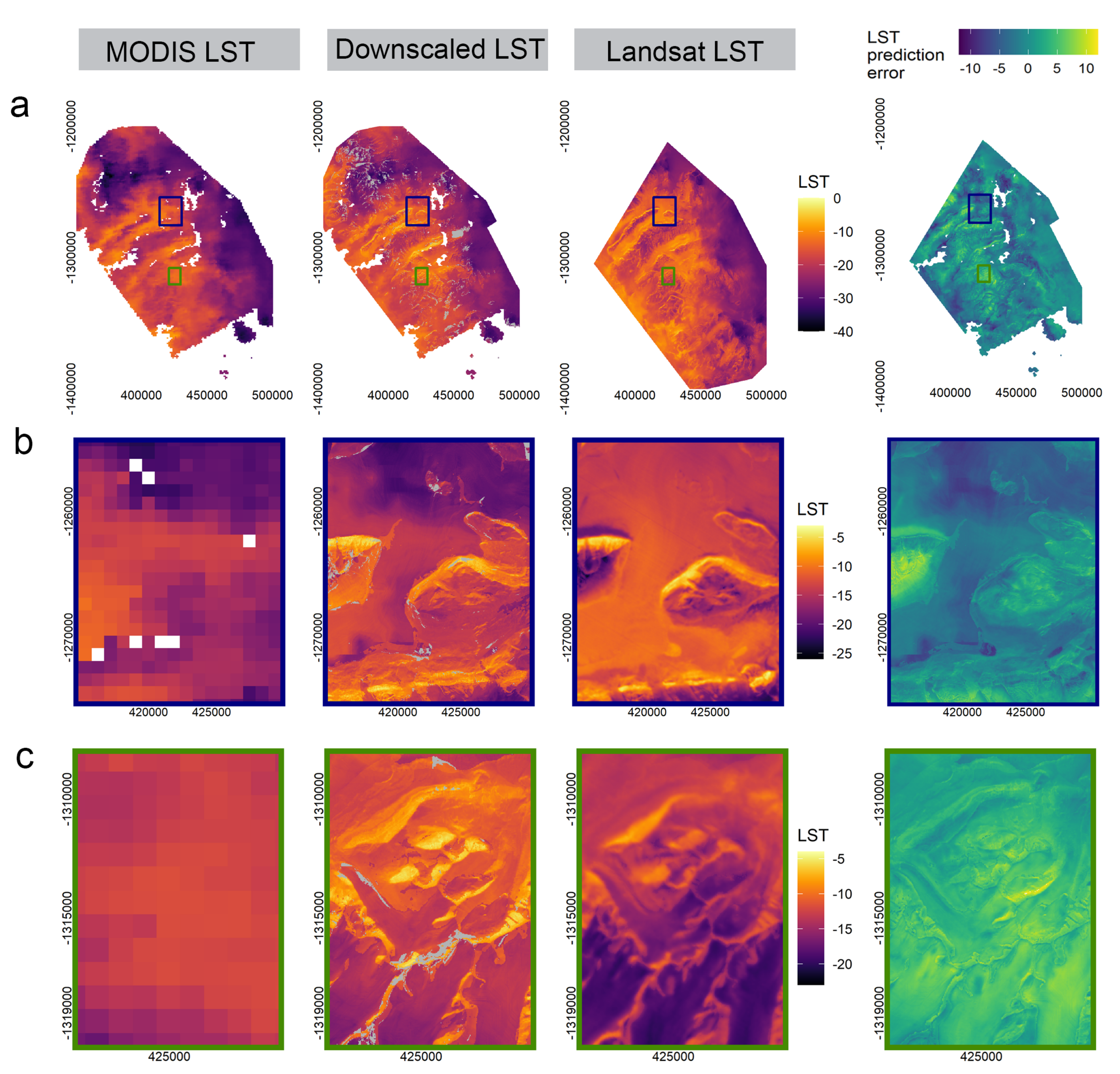
4. Results
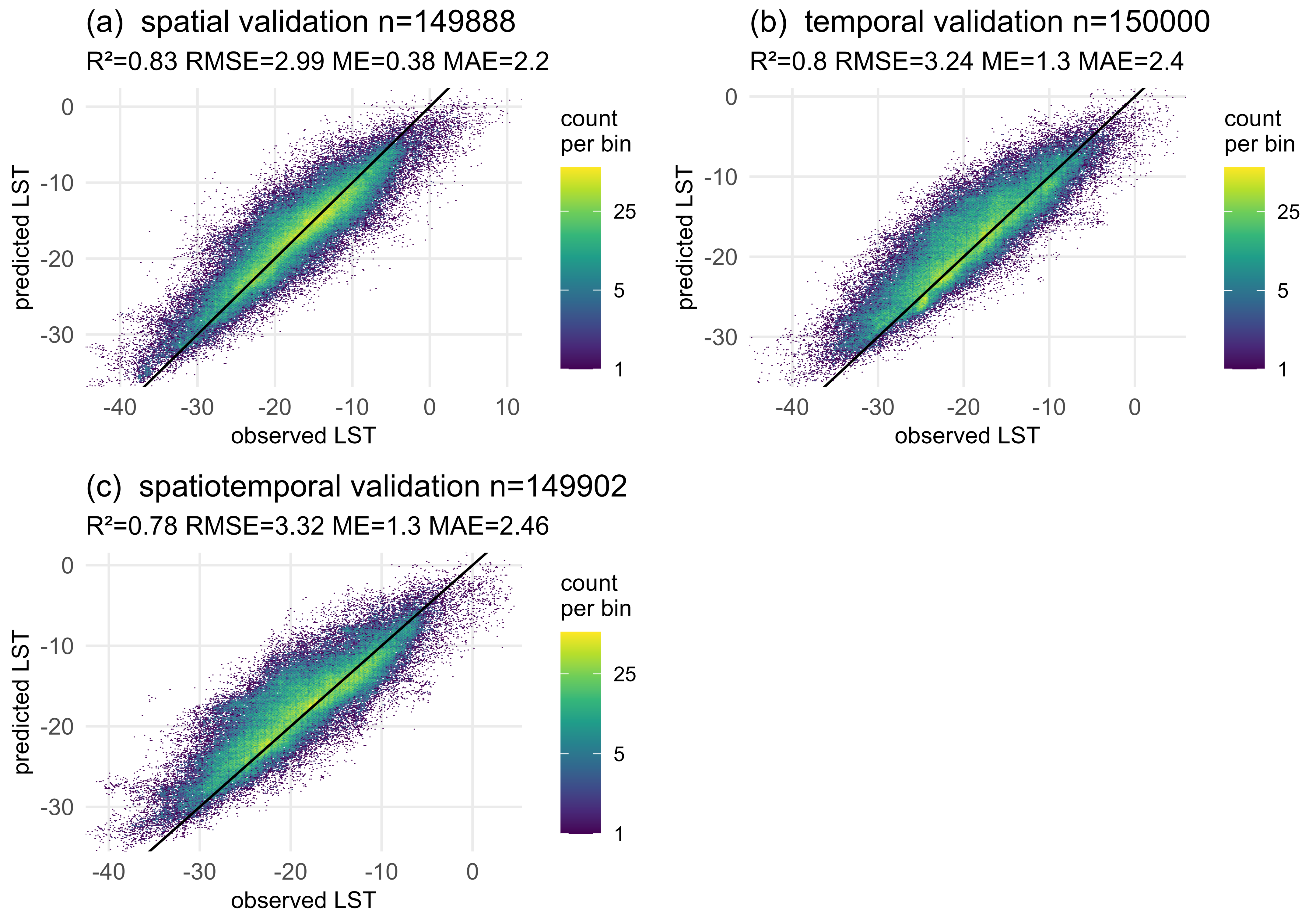
4.1. Model Selection and Evaluation
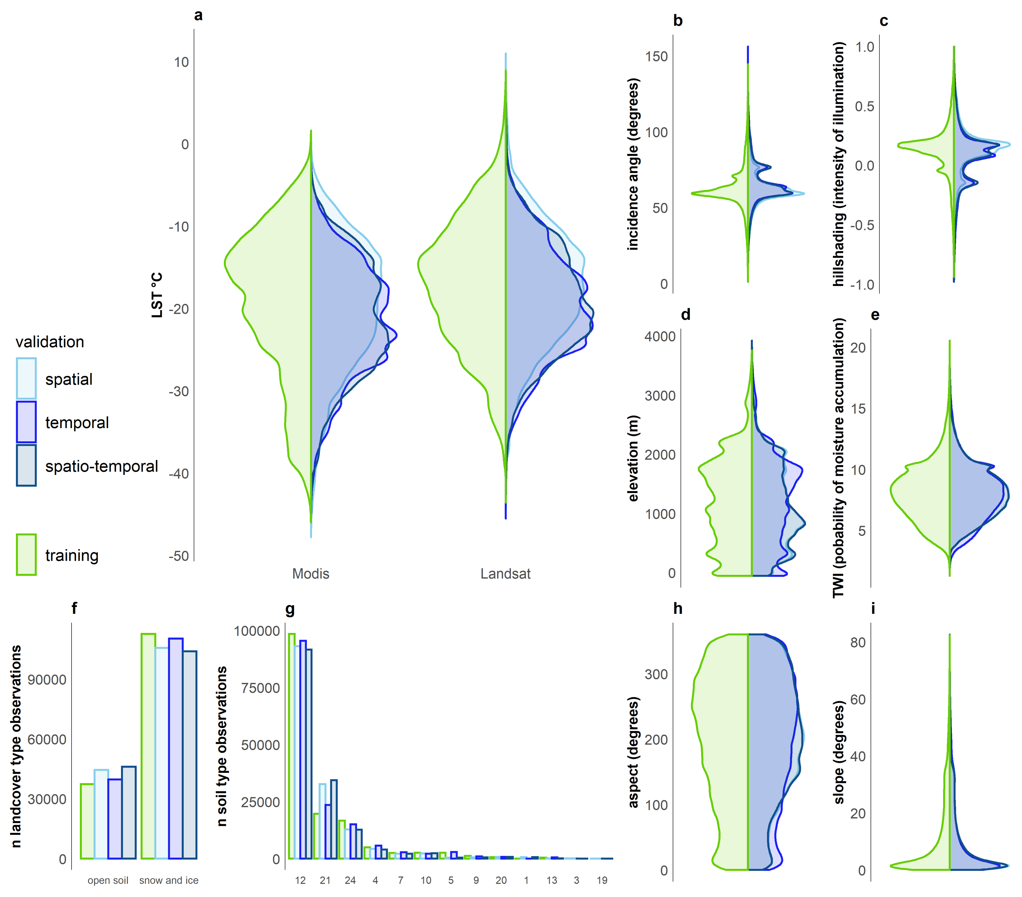
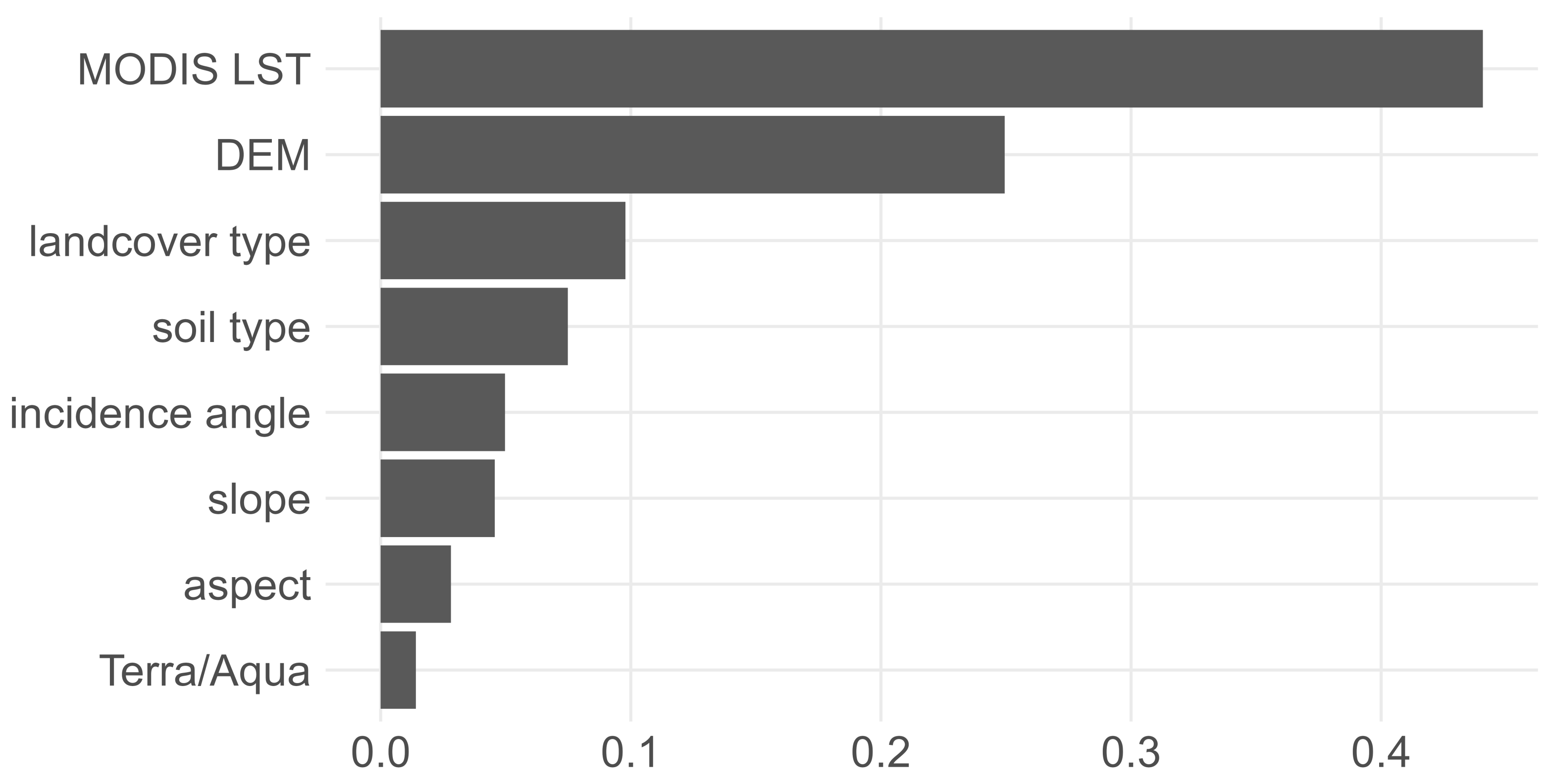
4.2. Selected Features
4.3. Area of Applicability
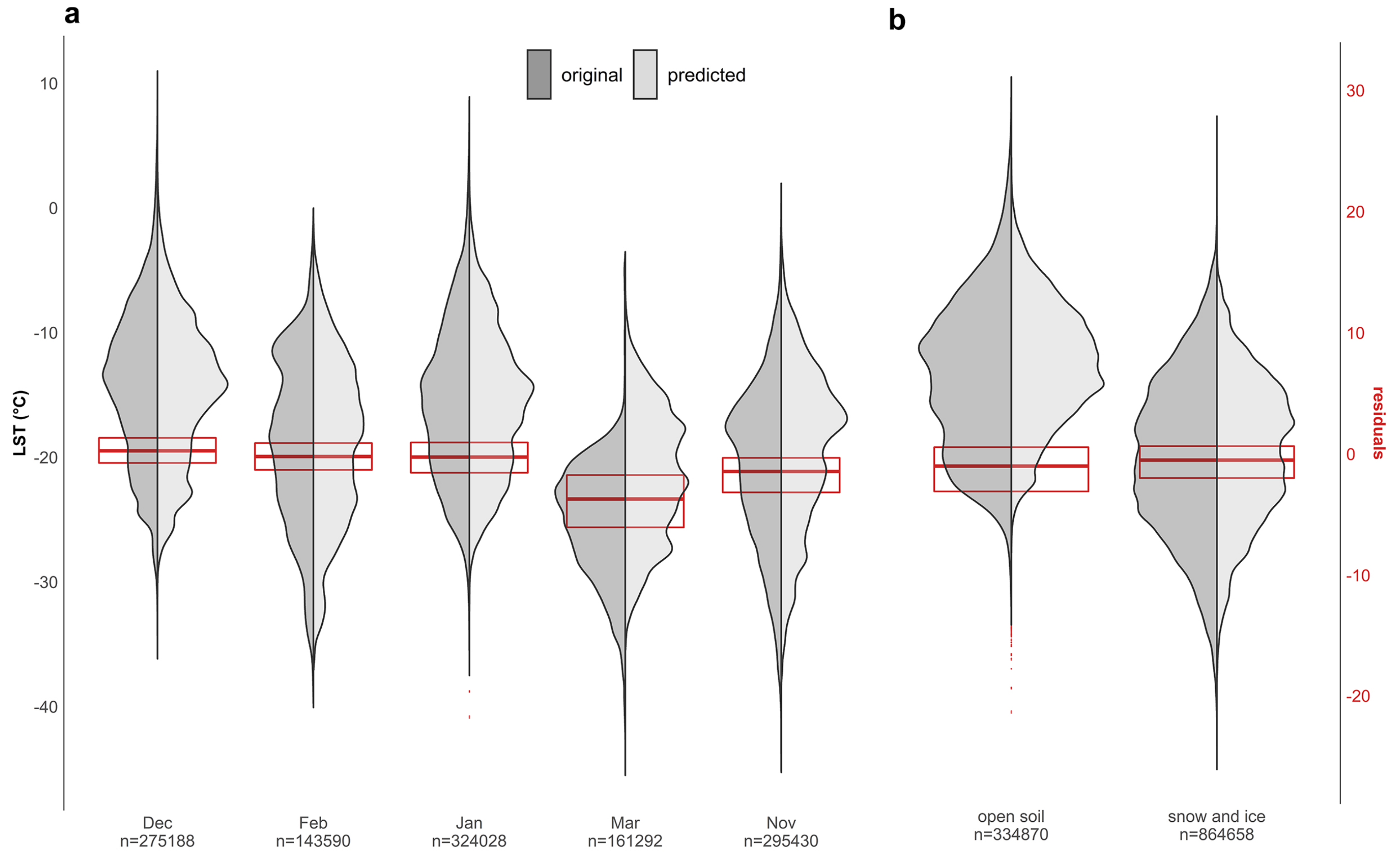
4.4. Performance over Time and Land Cover Types
5. Discussion
5.1. Variable Selection
5.2. Model Evaluation
5.3. Scope of Applicability
5.4. Comparison to Other Studies
5.5. Current Limitations and Future Perspectives of the Downscaled Data Set
6. Conclusions
Author Contributions
Funding
Data Availability Statement
Acknowledgments
Conflicts of Interest
Abbreviations
| LST | Land Surface Temperature |
| RF | Random Forest |
| GBM | Gradient Boosting Machine |
| NN | Neural Net |
| CV | Cross Validation |
| MDV | McMurdo Dry Valleys |
| TWI | Topographic Wetness Index |
| REMA | Reference Elevation Model of Antarctica |
| RAMP | Radarsat Antarctic Mapping Project Digital Elevation Model |
| RMSE | Root Mean Square Error |
| AOA | Area of Applicability |
| FFS | Forward Feature Selection |
References
- Zhao, W.; Duan, S.B.; Li, A.; Yin, G. A practical method for reducing terrain effect on land surface temperature using random forest regression. Remote Sens. Environ. 2019, 221, 635–649. [Google Scholar] [CrossRef]
- Yu, Y.; Liu, Y.; Yu, P. Land Surface Temperature Product Development for JPSS and GOES-R Missions. In Comprehensive Remote Sensing; Liang, S., Ed.; Elsevier: Amsterdam, The Netherlands, 2018; pp. 284–303. [Google Scholar] [CrossRef]
- Avdan, U.; Jovanovska, G. Algorithm for Automated Mapping of Land Surface Temperature Using LANDSAT 8 Satellite Data. J. Sens. 2016, 2016, 1480307. [Google Scholar] [CrossRef] [Green Version]
- Li, Z.L.; Tang, B.H.; Wu, H.; Ren, H.; Yan, G.; Wan, Z.; Trigo, I.F.; Sobrino, J.A. Satellite-derived land surface temperature: Current status and perspectives. Remote Sens. Environ. 2013, 131, 14–37. [Google Scholar] [CrossRef] [Green Version]
- Dash, P. Land Surface Temperature and Emissivity Retrieval from Satellite Measurements. Ph.D. Thesis, Universität Karlsruhe, Karlsruhe, Germany, 2004. [Google Scholar]
- Cammalleri, C.; Vogt, J. On the Role of Land Surface Temperature as Proxy of Soil Moisture Status for Drought Monitoring in Europe. Remote Sens. 2015, 7, 16849–16864. [Google Scholar] [CrossRef] [Green Version]
- Lee, J.R.; Raymond, B.; Bracegirdle, T.J.; Chadès, I.; Fuller, R.A.; Shaw, J.D.; Terauds, A. Climate change drives expansion of Antarctic ice-free habitat. Nature 2017, 547, 49. [Google Scholar] [CrossRef] [PubMed]
- Chown, S.L.; Clarke, A.; Fraser, C.I.; Cary, S.C.; Moon, K.L.; McGeoch, M.A. The changing form of Antarctic biodiversity. Nature 2015, 522, 431. [Google Scholar] [CrossRef] [PubMed]
- Fraser, C.I.; Morrison, A.K.; Hogg, A.M.; Macaya, E.C.; van Sebille, E.; Ryan, P.G.; Padovan, A.; Jack, C.; Valdivia, N.; Waters, J.M. Antarctica’s ecological isolation will be broken by storm-driven dispersal and warming. Nat. Clim. Chang. 2018, 8, 704. [Google Scholar] [CrossRef] [Green Version]
- Pattyn, F.; Ritz, C.; Hanna, E.; Asay-Davis, X.; DeConto, R.; Durand, G.; Favier, L.; Fettweis, X.; Goelzer, H.; Golledge, N.R.; et al. The Greenland and Antarctic ice sheets under 1.5 ∘C global warming. Nat. Clim. Chang. 2018, 8, 1053–1061. [Google Scholar] [CrossRef] [Green Version]
- Andriuzzi, W.S.; Adams, B.J.; Barrett, J.E.; Virginia, R.A.; Wall, D.H. Observed trends of soil fauna in the Antarctic Dry Valleys: Early signs of shifts predicted under climate change. Ecology 2018, 99, 312–321. [Google Scholar] [CrossRef]
- Lee, J.E.; Le Roux, P.C.; Meiklejohn, K.I.; Chown, S.L. Species distribution modelling in low-interaction environments: Insights from a terrestrial Antarctic system. Austral Ecol. 2013, 38, 279–288. [Google Scholar] [CrossRef]
- Gooseff, M.N.; Barrett, J.E.; Adams, B.J.; Doran, P.T.; Fountain, A.G.; Lyons, W.B.; McKnight, D.M.; Priscu, J.C.; Sokol, E.R.; Takacs-Vesbach, C.; et al. Decadal ecosystem response to an anomalous melt season in a polar desert in Antarctica. Nat. Ecol. Evol. 2017, 1, 1334–1338. [Google Scholar] [CrossRef]
- Kraaijenbrink, P.D.A.; Shea, J.M.; Litt, M.; Steiner, J.F.; Treichler, D.; Koch, I.; Immerzeel, W.W. Mapping Surface Temperatures on a Debris-Covered Glacier With an Unmanned Aerial Vehicle. Front. Earth Sci. 2018, 6, 64. [Google Scholar] [CrossRef] [Green Version]
- EROS. Collection-1 Landsat 8 OLI (Operational Land Imager) and TIRS (Thermal Infrared Sensor) Data Products. Available online: https://www.usgs.gov/centers/eros/science/usgs-eros-archive-landsat-archives-landsat-8-oli-operational-land-imager-and?qt-science_center_objects=0#qt-science_center_objects (accessed on 17 November 2021). [CrossRef]
- Tang, B.H.; Wang, J. A Physics-Based Method to Retrieve Land Surface Temperature From MODIS Daytime Midinfrared Data. IEEE Trans. Geosci. Remote Sens. 2016, 54, 4672–4679. [Google Scholar] [CrossRef]
- Zhan, W.; Chen, Y.; Zhou, J.; Wang, J.; Liu, W.; Voogt, J.; Zhu, X.; Quan, J.; Li, J. Disaggregation of remotely sensed land surface temperature: Literature survey, taxonomy, issues, and caveats. Remote Sens. Environ. 2013, 131, 119–139. [Google Scholar] [CrossRef]
- Agam, N.; Kustas, W.P.; Anderson, M.C.; Li, F.; Colaizzi, P.D. Utility of thermal sharpening over Texas high plains irrigated agricultural fields. J. Geophys. Res. 2007, 112, 1–10. [Google Scholar] [CrossRef] [Green Version]
- Khandelwal, S.; Goyal, R.; Kaul, N.; Mathew, A. Assessment of land surface temperature variation due to change in elevation of area surrounding Jaipur, India. Egypt. J. Remote Sens. Space Sci. 2018, 21, 87–94. [Google Scholar] [CrossRef]
- Stephen, H.; Ahmad, S.; Piechota, T.C. Land Surface Brightness Temperature Modeling Using Solar Insolation. IEEE Trans. Geosci. Remote Sens. 2010, 48, 491–498. [Google Scholar] [CrossRef]
- Zakšek, K.; Oštir, K.; Kokalj, Ž. Sky-View Factor as a Relief Visualization Technique. Remote Sens. 2011, 3, 398–415. [Google Scholar] [CrossRef] [Green Version]
- Pratt, D.A.; Ellyett, C.D. The thermal inertia approach to mapping of soil moisture and geology. Remote Sens. Environ. 1979, 8, 151–168. [Google Scholar] [CrossRef]
- Katurji, M.; Zawar-Reza, P.; Zhong, S. Surface layer response to topographic solar shading in Antarctica’s dry valleys. J. Geophys. Res. Atmos. 2013, 118, 12332–12344. [Google Scholar] [CrossRef]
- Stichbury, G.; Brabyn, L.; Allan Green, T.G.; Cary, C. Spatial modelling of wetness for the Antarctic Dry Valleys. Polar Res. 2011, 30, 6330. [Google Scholar] [CrossRef]
- Deardorff, J.W. Efficient prediction of ground surface temperature and moisture, with inclusion of a layer of vegetation. J. Geophys. Res. 1978, 83, 1889. [Google Scholar] [CrossRef] [Green Version]
- Keramitsoglou, I.; Kiranoudis, C.T.; Weng, Q. Downscaling Geostationary Land Surface Temperature Imagery for Urban Analysis. IEEE Geosci. Remote Sens. Lett. 2013, 10, 1253–1257. [Google Scholar] [CrossRef]
- Ebrahimy, H.; Azadbakht, M. Downscaling MODIS land surface temperature over a heterogeneous area: An investigation of machine learning techniques, feature selection, and impacts of mixed pixels. Comput. Geosci. 2019, 124, 93–102. [Google Scholar] [CrossRef]
- Hutengs, C.; Vohland, M. Downscaling land surface temperatures at regional scales with random forest regression. Remote Sens. Environ. 2016, 178, 127–141. [Google Scholar] [CrossRef]
- Zakšek, K.; Oštir, K. Downscaling land surface temperature for urban heat island diurnal cycle analysis. Remote Sens. Environ. 2012, 117, 114–124. [Google Scholar] [CrossRef]
- Stathopoulou, M.; Cartalis, C. Downscaling AVHRR land surface temperatures for improved surface urban heat island intensity estimation. Remote Sens. Environ. 2009, 113, 2592–2605. [Google Scholar] [CrossRef]
- Bechtel, B.; Zakšek, K.; Hoshyaripour, G. Downscaling Land Surface Temperature in an Urban Area: A Case Study for Hamburg, Germany. Remote Sens. 2012, 4, 3184–3200. [Google Scholar] [CrossRef] [Green Version]
- Doran, P.T.; Priscu, J.C.; Lyons, W.B.; Walsh, J.E.; Fountain, A.G.; McKnight, D.M.; Moorhead, D.L.; Virginia, R.A.; Wall, D.H.; Clow, G.D.; et al. Antarctic climate cooling and terrestrial ecosystem response. Nature 2002, 415, 517. [Google Scholar] [CrossRef]
- Cary, C.; Cowan, D.A.; Mcdonald, I. On the rocks: The microbiology of Antarctic dry valley soils. Nat. Rev. Microbiol. 2010, 8, 129–138. [Google Scholar] [CrossRef]
- Burkins, M.B.; Virginia, R.A.; Chamberlain, C.P.; Wall, D.H. Origin and distribution of soil organic matter in taylor valley, antarctica. Ecology 2000, 81, 2377–2391. [Google Scholar] [CrossRef]
- Virginia, R.A.; Wall, D.H. How Soils Structure Communities in the Antarctic Dry Valleys. BioScience 1999, 49, 973–983. [Google Scholar] [CrossRef]
- Yung, C.C.M.; Chan, Y.; Lacap, D.C.; Pérez-Ortega, S.; de Los Rios-Murillo, A.; Lee, C.K.; Cary, S.C.; Pointing, S.B. Characterization of chasmoendolithic community in Miers Valley, McMurdo Dry Valleys, Antarctica. Microb. Ecol. 2014, 68, 351–359. [Google Scholar] [CrossRef] [PubMed]
- Levy, J. How big are the McMurdo Dry Valleys? Estimating ice-free area using Landsat image data. Antarct. Sci. 2013, 25, 119–120. [Google Scholar] [CrossRef]
- Doran, P.T. Valley floor climate observations from the McMurdo dry valleys, Antarctica, 1986–2000. J. Geophys. Res. 2002, 107, 177. [Google Scholar] [CrossRef] [Green Version]
- Bertler, N.A.N. El Niño suppresses Antarctic warming. Geophys. Res. Lett. 2004, 31, 1–4. [Google Scholar] [CrossRef] [Green Version]
- R Core Team. R: A Language and Environment for Statistical Computing; R Core Team: Vienna, Austria, 2020. [Google Scholar]
- Schwalb-Willmann, J.; Fisser, H. getSpatialData: Get Different Kinds of Freely Available Spatial Datasets. R Package Version 0.1.1. 2020. Available online: http://www.github.com/16eagle/getSpatialData/ (accessed on 21 October 2021).
- Greenberg, J.A.; USGS ESPA. Espa.Tools: Wrappers for the USGS ESPA APIs and Earth Explorer; R Package Version 0.65/r35. 2018. Available online: https://R-Forge.R-project.org/projects/espa-tools/ (accessed on 21 October 2021).
- USGS. Landsat 8 OLI and TIRS Calibration Notices. 2017. Available online: https://www.usgs.gov/core-science-systems/nli/landsat/landsat-8-oli-and-tirs-calibration-notices (accessed on 17 November 2021).
- Wan, Z. MODIS Land-Surface Temperature Algorithm Theoretical Basis Document: Version 3.3. Ph.D. Thesis, Institute for Computational Earth System Science, University of California, Santa Barbara, USA, 1999. [Google Scholar]
- Burton-Johnson, A.; Black, M.; Fretwell, P.T.; Kaluza-Gilbert, J. An automated methodology for differentiating rock from snow, clouds and sea in Antarctica from Landsat 8 imagery: A new rock outcrop map and area estimation for the entire Antarctic continent. Cryosphere 2016, 10, 1665–1677. [Google Scholar] [CrossRef] [Green Version]
- Kondo, J.; Yamazawa, H. Measurement of snow surface emissivity. Bound.-Layer Meteorol. 1986, 34, 415–416. [Google Scholar] [CrossRef]
- Mira, M.; Valor, E.; Boluda, R.; Caselles, V.; Coll, C. Influence of soil water content on the thermal infrared emissivity of bare soils: Implication for land surface temperature determination. J. Geophys. Res. 2007, 112. [Google Scholar] [CrossRef] [Green Version]
- Wan, Z. MODIS Land Surface Temperature Products User’s Guide. Available online: https://lpdaac.usgs.gov/documents/118/MOD11_User_Guide_V6.pdf (accessed on 17 November 2021).
- Greenberg, J.; Mattiuzzi, M. gdalUtils: Wrappers for the Geospatial Data Abstraction Library (GDAL) Utilities. R Package Version 2.0.3.2. 2020. Available online: https://CRAN.R-project.org/package=gdalUtils (accessed on 21 October 2021).
- Wan, Z.; Hook, S.; Hulley, G. MOD11_L2 MODIS/Terra Land Surface Temperature/Emissivity 5-Min L2 Swath 1 km V006. Available online: https://lpdaac.usgs.gov/products/mod11_l2v006/ (accessed on 17 November 2021). [CrossRef]
- Wan, Z.; Hoo, S.; Hulley, G. MYD11_L2 MODIS/Aqua Land Surface Temperature/Emissivity 5-Min L2 Swath 1 km V006. Available online: https://lpdaac.usgs.gov/products/myd11_l2v006/ (accessed on 17 November 2021). [CrossRef]
- Howat, I.M.; Porter, C.; Smith, B.E.; Noh, M.J.; Morin, P. The Reference Elevation Model of Antarctica. Cryosphere 2019, 13, 665–674. [Google Scholar] [CrossRef] [Green Version]
- Liu, H.; Jezek, K.C.; Li, B.; Zhao, Z.; Liu, H. Radarsat Antarctic Mapping Project Digital Elevation Model; Version 2. 2015. Available online: https://nsidc.org/data/NSIDC-0082/versions/2 (accessed on 17 November 2021). [CrossRef]
- Bockheim, J.G.; McLeod, M. Soil distribution in the McMurdo Dry Valleys, Antarctica. Geoderma 2008, 144, 43–49. [Google Scholar] [CrossRef]
- Kelley, D.; Richards, C. Oce: Analysis of Oceanographic Data. R Package Version 1.2-0. 2020. Available online: https://CRAN.R-project.org/package=oce (accessed on 21 October 2021).
- Seyednasrollah, B. Solrad: To Calculate Solar Radiation and Related Variables Based on Location, Time and Topographical Conditions. R Package Version 1.0.0. 2018. Available online: http://doi.org/10.5281/zenodo.1006383 (accessed on 21 October 2021). [CrossRef]
- Hijmans, R.J. Raster: Geographic Data Analysis and Modeling. R Package Version 3.4-13. 2020. Available online: https://CRAN.R-project.org/package=raster (accessed on 21 October 2021).
- Böhner, J.; Selige, T. Spatial Prediction of Soil Attributes Using Terrain Analysis and Climate Regionalisation. In SAGA—Analysis and Modelling Applications; Böhner, J., McCloy, K.R., Strobl, J., Eds.; Verlag Erich Goltze GmbH: Göttingen, Germany, 2006; Volume 115, pp. 13–27. [Google Scholar]
- Meyer, H.; Pebesma, E. Predicting into unknown space? Estimating the area of applicability of spatial prediction models. Methods Ecol. Evol. 2021, 12, 1620–1633. [Google Scholar] [CrossRef]
- Meyer, H. CAST: ‘caret’ Applications for Spatial-Temporal Models. R Package Version 0.5.1. 2020. Available online: https://CRAN.R-project.org/package=CAST (accessed on 21 October 2021).
- Minasny, B.; McBratney, A.B. A conditioned Latin hypercube method for sampling in the presence of ancillary information. Comput. Geosci. 2006, 32, 1378–1388. [Google Scholar] [CrossRef]
- Roudier, P. Clhs: A R Package for Conditioned Latin Hypercube Sampling. R Package. 2011. Available online: https://github.com/pierreroudier/clhs/ (accessed on 21 October 2021).
- Meyer, H.; Katurji, M.; Appelhans, T.; Müller, M.; Nauss, T.; Roudier, P.; Zawar-Reza, P. Mapping Daily Air Temperature for Antarctica Based on MODIS LST. Remote Sens. 2016, 8, 732. [Google Scholar] [CrossRef] [Green Version]
- Liaw, A.; Wiener, M. Classification and Regression by randomForest. 2002. Available online: https://cran.r-project.org/doc/Rnews/Rnews_2002-3.pdf (accessed on 17 November 2021).
- Greenwell, B.; Boehmke, B.; Cunningham, J.; GBM Developers. Gbm: Generalized Boosted Regression Models. R Package Version 2.1.8. 2020. Available online: https://CRAN.R-project.org/package=gbm (accessed on 21 October 2021).
- Venables, W.N.; Ripley, B.D. Modern Applied Statistics with S, 4th ed.; Springer: New York, NY, USA, 2002. [Google Scholar]
- Kuhn, M. Caret: Classification and Regression Training. R Package Version 6.0-86. 2020. Available online: https://CRAN.R-project.org/package=caret (accessed on 21 October 2021).
- Ploton, P.; Mortier, F.; Réjou-Méchain, M.; Barbier, N.; Picard, N.; Rossi, V.; Dormann, C.; Cornu, G.; Viennois, G.; Bayol, N.; et al. Spatial validation reveals poor predictive performance of large-scale ecological mapping models. Nat. Commun. 2020, 11, 4540. [Google Scholar] [CrossRef] [PubMed]
- Meyer, H.; Reudenbach, C.; Hengl, T.; Katurji, M.; Nauss, T. Improving performance of spatio-temporal machine learning models using forward feature selection and target-oriented validation. Environ. Model. Softw. 2018, 101, 1–9. [Google Scholar] [CrossRef]
- Sismanidis, P.; Keramitsoglou, I.; Bechtel, B.; Kiranoudis, C. Improving the Downscaling of Diurnal Land Surface Temperatures Using the Annual Cycle Parameters as Disaggregation Kernels. Remote Sens. 2017, 9, 23. [Google Scholar] [CrossRef] [Green Version]
- Speirs, J.C.; Steinhoff, D.F.; McGowan, H.A.; Bromwich, D.H.; Monaghan, A.J. Foehn Winds in the McMurdo Dry Valleys, Antarctica: The Origin of Extreme Warming Events. J. Clim. 2010, 23, 3577–3598. [Google Scholar] [CrossRef] [Green Version]
- Zawar-Reza, P.; Katurji, M.; Soltanzadeh, I.; Dallafior, T.; Zhong, S.; Steinhoff, D.; Storey, B.; Cary, S.C. Pseudovertical Temperature Profiles Give Insight into Winter Evolution of the Atmospheric Boundary Layer over the McMurdo Dry Valleys of Antarctica. J. Appl. Meteorol. Climatol. 2013, 52, 1664–1669. [Google Scholar] [CrossRef] [Green Version]
- Cassano, J.J.; Nigro, M.A.; Seefeldt, M.W.; Katurji, M.; Guinn, K.; Williams, G.; DuVivier, A. Antarctic atmospheric boundary layer observations with the Small Unmanned Meteorological Observer (SUMO): Preprint. Earth Syst. Sci. Data 2020, 13, 969–982. [Google Scholar] [CrossRef]
- Katurji, M.; Khan, B.; Sprenger, M.; Datta, R.; Joy, K.; Zawar-Reza, P.; Hawes, I. Meteorological Connectivity from Regions of High Biodiversity within the McMurdo Dry Valleys of Antarctica. J. Appl. Meteorol. Climatol. 2019, 58, 2437–2452. [Google Scholar] [CrossRef]


| Predictor Variable | Connection to High Resolution LST | Original Spatial Resolution (m) | Temporal Resolution | Source |
|---|---|---|---|---|
| MODIS LST | variable to be downscaled | 1000 | subdaily | [50,51] |
| DEM | meteorological lapse | 8 (200 for filling NA) | static | REMA [52] & RAMP [53] |
| incidence angle | solar insolation | 8 | subdaily | DEM + MODIS capturing time |
| hillshading | direct or diffuse solar insolation | 8 | subdaily | DEM + MODIS capturing time |
| slope | possibility for water accumulation | 8 | static | DEM |
| aspect | direct or diffuse insolation for different periods of time per day | 8 | static | DEM |
| land surface type | albedo | 30 | static | Landsat classification [45] |
| soil map | water retention capacity of soil types and albedo | from vector | static | Landcare Research [54] |
| TWI | water content affects LST, TWI proxi for hydrologic routing | 8 | static | DEM via SAGA TWI algorithm |
| Terra/Aqua | Acquisitions from Terra are temporally further apart from the response variable | whole scene | spatial constant per scene | MODIS filename |
| Algorithm (Caret Method) | Hyperparameter | Tested Value Final Model | Optimal Value Final Model |
|---|---|---|---|
| Random Forest (rf) | mtry | 2 to 4 with increment 1 | 2 |
| Gradient Boosting (gbm) | number of trees max depth of interactions shrinkage min observations in terminal nodes | 100 to 500 with increment 100 3 to 14 with increment 2 0.01, 0.05, 0.1 10 | 500 3 0.01 10 |
| Artificial Neural Net (nnet) | size decay | 1, 2, 3, 5, 10, 20 0.5, 0.1, 1 × 10 bis 1 × 10 | 20 0.0001 |
| Spatial | Temporal | Spatio-Temporal | ||||
|---|---|---|---|---|---|---|
| R | RMSE | R | RMSE | R | RMSE | |
| RF | 0.83 | 2.99 | 0.80 | 3.24 | 0.78 | 3.32 |
| NN | 0.8 | 3.26 | 0.75 | 3.69 | 0.73 | 3.74 |
| GBM | 0.73 | 3.68 | 0.72 | 3.70 | 0.7 | 3.58 |
Publisher’s Note: MDPI stays neutral with regard to jurisdictional claims in published maps and institutional affiliations. |
© 2021 by the authors. Licensee MDPI, Basel, Switzerland. This article is an open access article distributed under the terms and conditions of the Creative Commons Attribution (CC BY) license (https://creativecommons.org/licenses/by/4.0/).
Share and Cite
Lezama Valdes, L.-M.; Katurji, M.; Meyer, H. A Machine Learning Based Downscaling Approach to Produce High Spatio-Temporal Resolution Land Surface Temperature of the Antarctic Dry Valleys from MODIS Data. Remote Sens. 2021, 13, 4673. https://doi.org/10.3390/rs13224673
Lezama Valdes L-M, Katurji M, Meyer H. A Machine Learning Based Downscaling Approach to Produce High Spatio-Temporal Resolution Land Surface Temperature of the Antarctic Dry Valleys from MODIS Data. Remote Sensing. 2021; 13(22):4673. https://doi.org/10.3390/rs13224673
Chicago/Turabian StyleLezama Valdes, Lilian-Maite, Marwan Katurji, and Hanna Meyer. 2021. "A Machine Learning Based Downscaling Approach to Produce High Spatio-Temporal Resolution Land Surface Temperature of the Antarctic Dry Valleys from MODIS Data" Remote Sensing 13, no. 22: 4673. https://doi.org/10.3390/rs13224673
APA StyleLezama Valdes, L.-M., Katurji, M., & Meyer, H. (2021). A Machine Learning Based Downscaling Approach to Produce High Spatio-Temporal Resolution Land Surface Temperature of the Antarctic Dry Valleys from MODIS Data. Remote Sensing, 13(22), 4673. https://doi.org/10.3390/rs13224673