Abstract
For monitoring protected forest landscapes over time it is essential to follow changes in tree species composition and forest dynamics. Data driven remote sensing methods provide valuable options if terrestrial approaches for forest inventories and monitoring activities cannot be applied efficiently due to restrictions or the size of the study area. We demonstrate how species can be detected at a single tree level utilizing a Random Forest (RF) model using the Black Forest National Park as an example of a Central European forest landscape with complex relief. The classes were European silver fir (Abies alba, AA), Norway spruce (Picea abies, PA), Scots pine (Pinus sylvestris, PS), European larch (Larix decidua including Larix kampferii, LD), Douglas fir (Pseudotsuga menziesii, PM), deciduous broadleaved species (DB) and standing dead trees (snags, WD). Based on a multi-temporal (leaf-on and leaf-off phenophase) and multi-spectral mosaic (R-G-B-NIR) with 10 cm spatial resolution, digital elevation models (DTM, DSM, CHM) with 40 cm spatial resolution and a LiDAR dataset with 25 pulses per m2, 126 variables were derived and used to train the RF algorithm with 1130 individual trees. The main objective was to determine a subset of meaningful variables for the RF model classification on four heterogeneous test sites. Using feature selection techniques, mainly passive optical variables from the leaf-off phenophase were considered due to their ability to differentiate between conifers and the two broader classes. An examination of the two phenological phases (using the difference of the respective NDVIs) is important to clearly distinguish deciduous trees from other classes including snags (WD). We also found that the variables of the first derivation of NIR and the tree metrics play a crucial role in discriminating PA und PS. With this unique set of variables some classes can be differentiated more reliably, especially LD and DB but also AA, PA and WD, whereas difficulties exist in identifying PM and PS. Overall, the non-parametric object-based approach has proved to be highly suitable for accurately detecting (OA: 89.5%) of the analyzed classes. Finally, the successful classification of complex 265 km2 study area substantiates our findings.
1. Introduction
Tree species composition, to a degree, shapes the habitat for forest dwelling species within a forest landscape and is therefore an essential indicator for the assessment of forest biodiversity conservation. Approaches to assess tree species composition using remote sensing techniques in forest management are common due to their cost effectiveness and efficiency [1,2,3].
There are three more reasons why using remote sensing is especially relevant for protected areas. The first and main reason is that protected areas of the IUCN Category I and II prioritize the protection of and learning from natural dynamics and processes [4]. Therefore, any disturbance by humans in these strictly protected areas, even by field crews collecting data, should be strictly limited. For this reason, classical terrestrial forest inventories, providing information about structure and tree species composition are restricted. This is also the case in our study area, the Black Forest National Park (BFNP) in southwest Germany.
Major natural processes that happen on larger scales over time, will often result in tree species composition changes [5] and this is the second reason for applying landscape level monitoring using remote sensing. For example, in Central Europe this change in forest tree species is most likely driven by blowdown [6] followed by bark beetle outbreaks but is also due to the effects of climate change, i.e., longer and more frequent droughts [7]. Therefore, the efficient and accurate detection of individual tree species on a landscape scale is essential for monitoring the changes. In the Black Forest, as in other Central European mountain landscapes, the human impact, especially forestry activities often resulted in forest composition becoming increasingly conifer dominated [8]. Monitoring changes in tree species composition in these previously managed forests will allows us to quantify the effect of the strict protection measures initiated within the BFNP over time.
To be able to quantify the impact of these landscape level changes on biodiversity in the BFNP, because of the protection of natural processes, is the third reason why remote sensing techniques are important. To capture individual tree information enables us to link patterns and processes at a landscape level combined with plot-based collected ecological data. Consequently, this allows for the identification of landscape level changes on organism groups and their interactions on a much finer scale.
Although remote sensing techniques have long been used in forest inventories, there are constantly new methods emerging due to the increasing availability of high-resolution data [9]. This development is also reflected in the more elaborate and accurate processing techniques available to detect specific objects of interest, such as identifying the species of individual trees. According to the comprehensive review on tree species classification studies from remotely sensed data of Fassnacht et al. [3], there are already a large and growing number of competing approaches. They reveal that research is still required to produce tree species inventories on a large geographic scale. In addition, the studies emphasized the need for evidence-based results from real and non-idealized test sites and for studies examining the causes of varying attributes.
Many relevant tree attributes vary seasonally in forests and, due to the important role of foliage cover [10,11], studies that primarily focus on such seasonally changing variables, can be considered particularly valuable to classify individual tree species. For example, Gara et al. [12] showed that different leaf traits influence the results of tree species classification when using satellite images.
Studies which address such seasonal tree characteristics often combine different approaches [13] and apply them to as high-resolution data as possible or at multi-scales [1]. Especially the complementary use of multiple high-resolution data, in addition to satellite images, seems promising for the classification of trees species, since the combined use of multiple data resolution can prevent the negative effects of spectral overlaps [14]. In summary, the literature reveals that in particular, a combination of various data sources, the study of seasonal effects and an accentuation of canopy characteristics are important, when the other characteristics hardly differ.
Recently, studies have systematically investigated the potential that combining various data sources has on the detection of tree species. Besides airborne hyperspectral imagery [15,16,17,18,19,20], derivatives from LiDAR airborn laser scan were often recommended for this purpose [10,21]. LiDAR return metrics are usually not analyzed individually to assess tree species composition. Instead, they are often combined with data from common passive remote sensing sources, generally R-G-B and IR bands of orthoimages. The benefit of such complementary approaches is a significant increase in accuracy [22,23]. Given the challenges posed by dense mixed temperate forests, it was shown that a multi-data approach is promising for achieving single tree delineation if an algorithm is implemented which uses only the most relevant variables of high dimensional features [24].
Considering variable reduction based on multi-data approaches, supervised deep learning methods offer effective solutions. Many studies [17,25,26,27] showed that non-parametric algorithms learn how to recognize promising variables based on trained patterns. This approach was supported in a review on deep leaning applications using remote sensing by Ma et al. [28]. Using an unmanned aerial vehicle (UAV) for data collection is another trend towards species classification of individual trees. Also, for the evaluation of the data generated, deep learning techniques are now often used to identify meaningful patterns [29]. Besides Support Vector Machines (SVM) [17,25,26,27], especially the Random Forest algorithm (RF) [30,31] is receiving increasing attention because of its highly effective decision trees for class prediction, with many possible applications in remote sensing [32,33,34,35]; for example to classify tree species [20,21,36]. This technique is largely independent of the datasets used.
Although tree species classification methods have been extensively studied, there is still a need to identify the best data sources, variables and techniques to accurately identify the species of an individual tree. Beyond the contribution made to the scientific discourse, such findings are particularly useful for practical applications. For example, to monitor changes in tree species composition due to natural forest dynamics in protected forest landscapes. Additionally, further empirical evidence contributes to the body of experience regarding cost-effectiveness and the most promising data sets.
The objective of this study was to evaluate the efficiency of the non-parametric Random Forest algorithm to detect the species of individual trees in a Central European forest landscape based on multi-source data sets and their derivatives. Specifically, 10 cm resolution multispectral 16-bit-mosaics (R-G-B-NIR) and LiDAR datasets attributed by 25 pulses per m2 were used. This approach, that we used, was meant to detect Norway spruce (Picea abies, PA), European silver fir (Abies alba, AA), Scots pine (Pinus sylvestris, PS), the introduced species European larch (Larix decidua including Larix kampferii, LD), and Douglas fir (Pseudotsuga menziesii, PM), deciduous broadleaved species (DB is not further differentiated), as well as standing dead trees from here on referred to as snags (WD).
Using the BFNP as an example, the following research questions were addressed:
- 1.
- Which variables are particularly meaningful for the differentiation and detection of the conifer species and the two broader structural classes?
- 2.
- Which species can be differentiated from each other with high rates of accuracy?
With this study, we provide a rare example of a practical application to an existing landscape with all of the methodological challenges that come with it.
2. Materials and Methods
2.1. Study Area: The Black Forest National Park and Surroundings
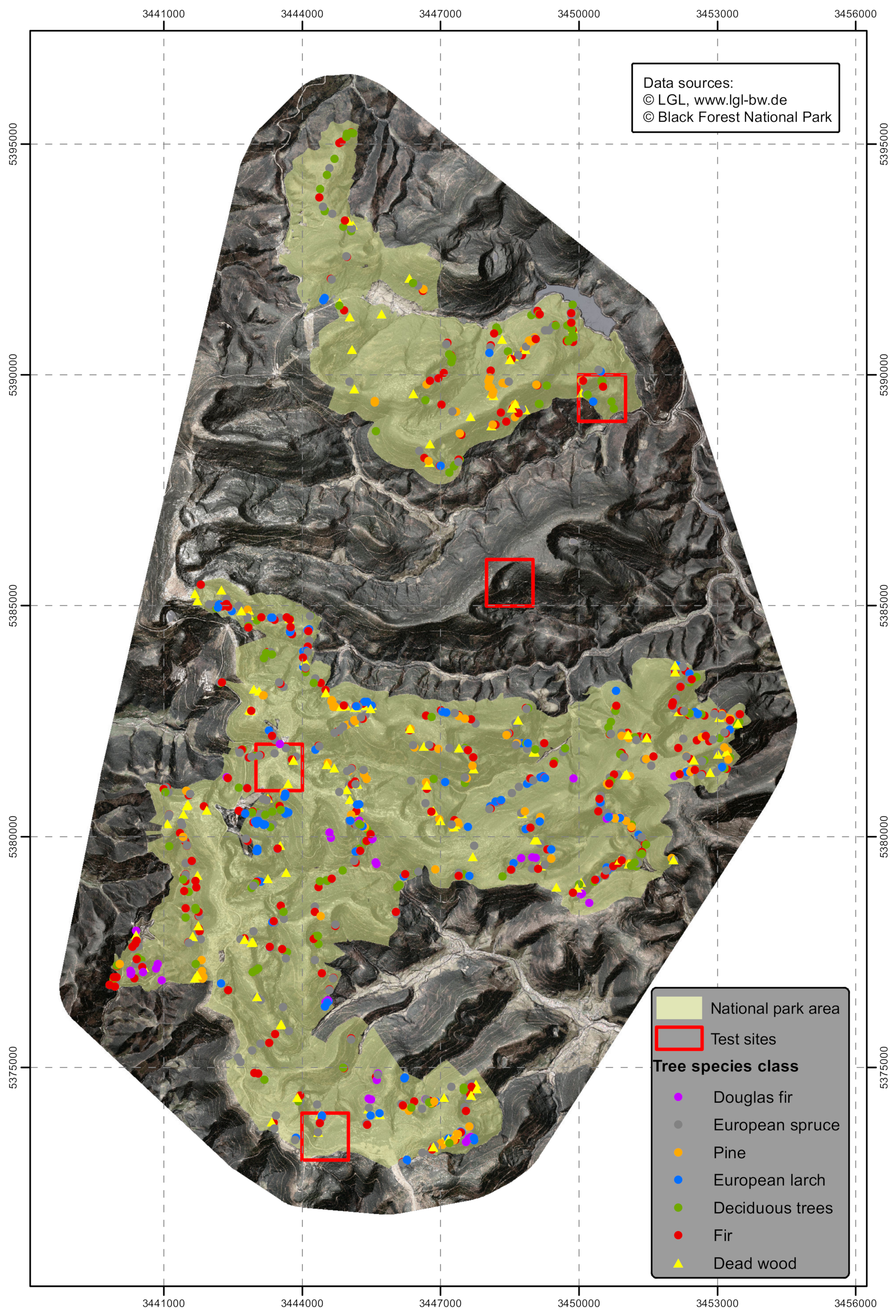
The study area with a size of 265 km2 is located in Baden-Württemberg, a federal state in the southwest of Germany includes the BFNP and adjacent areas (Figure 1). The temperate mixed mountain forests occur over a wide elevation range (from 400 to 1150 m, but mainly grow in a montane belt from 600 to 1000 m) and that is characterized by acidic and nutrient poor soils developed on sandstone and metamorphic bedrock [37,38].
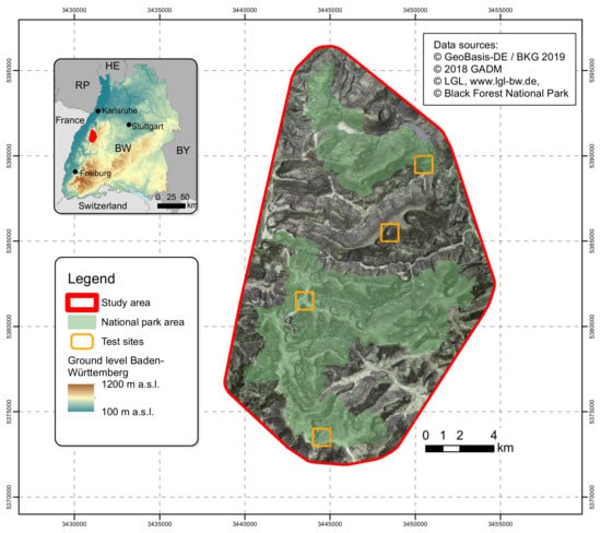
Figure 1.
Map of the study area and location of test sites.
The area is located in the humid mid-latitudes, influenced by a changeable oceanic climate with mild summers and cool winters [39]. Due to the west wind, at the eastern shoulder of the Upper Rhine Rift Valley, prevalent in the study area, there are higher precipitation rates (above 2000 mm/a) and lower mean temperature fluctuations (5 °C and 8 °C) during the year than in other areas of the Black Forest [40]. Nevertheless, there are distinct seasons and deciduous trees are seasonally in leaf-on or leaf-off condition. The current forest tree species are dominantly conifer species, the result of centuries of forestry practices. Approximately half of the study area is covered by the BFNP (Figure 1) where the protection of natural forest dynamics has recently been instituted. It is therefore expected that the tree species composition will change depending on natural disturbances like blowdown and the impacts of climate change like extended droughts.
2.2. Raw Data Sets
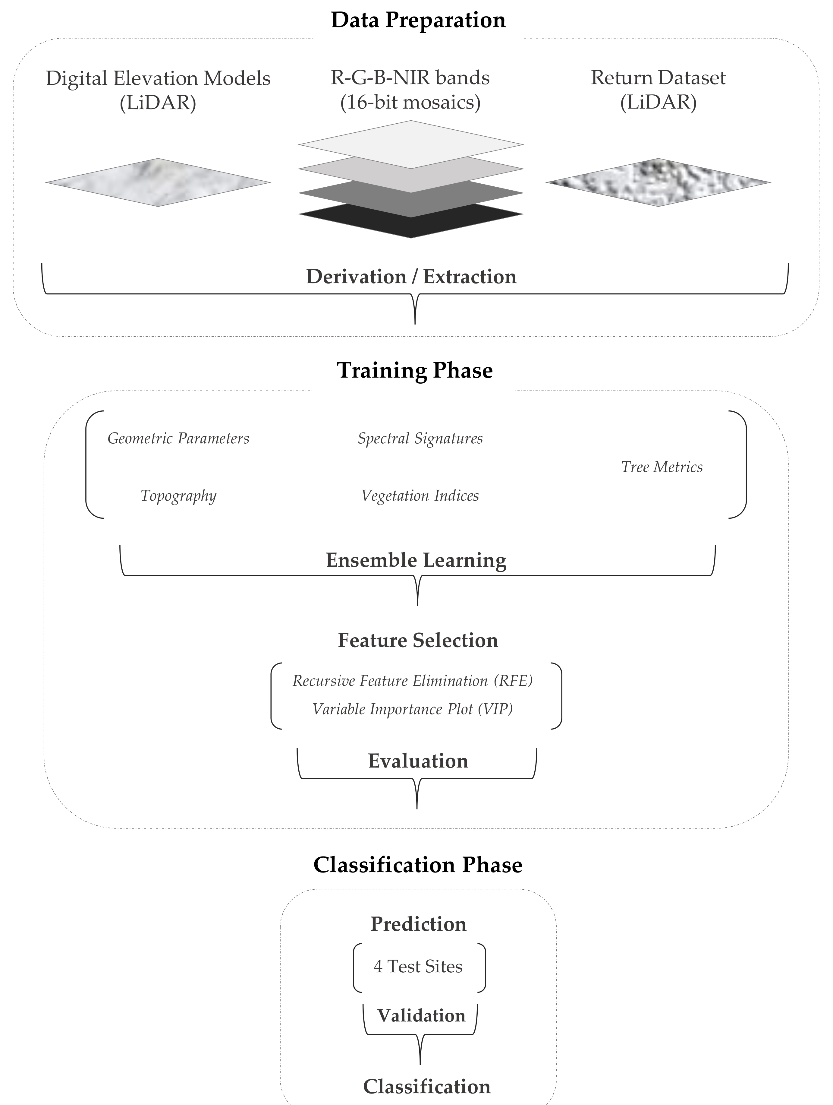
The original data sets include passive-optically obtained multispectral 16-bit-mosaics (R-G-B-NIR bands), actively obtained laser scan return data sets (LiDAR) and their derivatives (Figure 2). The multispectral mosaics are available for the entire study area and for two phenological phases (leaf-on in summer 2014 and leaf-off in spring 2015), in order to identify deciduous broadleaved species and larch. The four wavelength ranges (full width at half maximum) represent both phenophases: blue (450–520 nm), green (510–570 nm), red (580–680 nm) and near infrared (710–830 nm). They were taken by two airborne cameras, an UltraCam Xp (leaf-on) on on 17 July 2014 and an UltraCam Eagle (leaf-off) on 16 April 2015 flying at an average altitude of 4300 feet. LiDAR was acquired on on 29 April 2015 onboard aircraft at an average altitude of 2800 feet using a Riegl VQ-780i scanner at a density of 25 pulses per m2 in the near infrared wavelength.
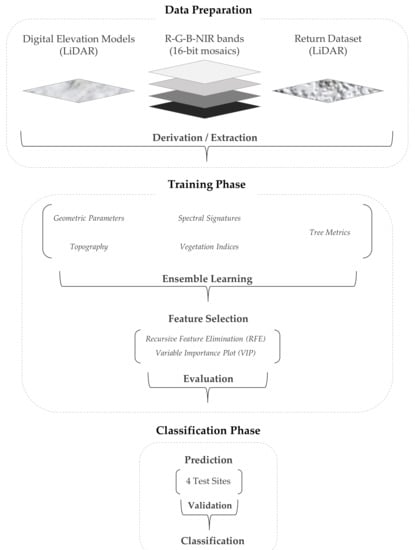
Figure 2.
Overview of data processing: First, the raw data were prepared in order to derive a number of categories consisting of attributes and potential variables. Second, during the training phase, the model parameters were tuned and the most significant variables were identified through feature selection methods. Last, the best-fitting model was applied to detect individual conifer species, the broad-leaved classes and snags in the test sites and after a comprehensive validation to the entire study area.
True Digital Orthophotos (TDOP) with absolute height and position data could be derived due to a high overlap (80% forward overlap. i.e., between photos along the same flight line, 60% lateral overlap, i.e., between photos on adjacent flight lines) based on the overlapping parameters. In addition, the use of TDOP enabled the co-registration of a tree’s highest point.
The multispectral sensors were calibrated before the flight, however as the processing of stereo images into TDOP included radiometric adjustment, a conversion into reflectance was not considered useful. LiDAR data acquired during the leaf-off phase in spring 2015 had been pre-processed into datasets of (1) 3D point clouds of returns, (2) surfaces of 40 cm spatial resolution including Digital Terrain Model (DTM) and Digital Surface Model (DSM) as well as (3) individual tree crown delineation polygons using the software TreesVIS [41]. The raw data set contains only trees with a minimum height of 15 m and a canopy area of 10 m2. Forest structure classification was adapted from O’Hara et al. [42] and Falkowski et al. [43]. In total more than 3 million trees within the BFNP were included.
2.3. Data Preparation
First, individual trees that represent the species and the species composition of the entire area had to be identified. The individual trees are used as a basis to train the RF algorithm and to determine relevant variables necessary to classify the trees in the study area. To make sure that the sampled trees (height ≥15 m and canopy area ≥10 m2) represent the full range of variation, the area was divided up into strips and visually interpreted using stereoscopic aerial photos.
As result, a training set of 1130 trees regularly distributed over the whole area were selected and identified to represent the previously defined classes. The frequency within the selected classes was similar to the species distribution in the forest inventory done prior to the national park designation. In order to have sufficient training data available for rare tree classes (e.g., Douglas fir), they had to be overrepresented in the training data set compared to frequently occurring tree classes (e.g., Norway spruce, silver fir). The training data set consisted of 273 Norway spruce (PA), 249 European silver fir (AA), 132 Scots pine (PS), 128 European larch (LD), 41 Douglas fir (PM), 163 deciduous broadleaved trees (DB), 146 individual standing snags (WD, (Figure 3)).
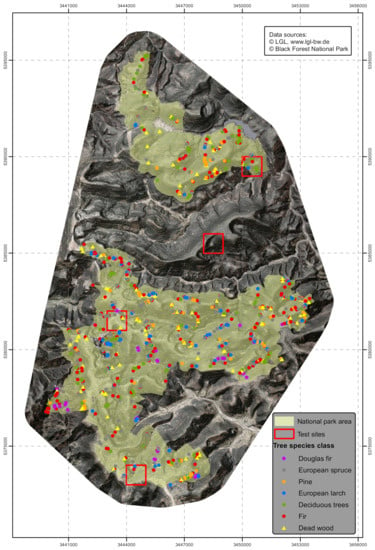
Figure 3.
The location of the trees used as training dataset within the study area.
The descriptive attribute values of the canopies were aggregated within a 1.7 m radial buffer from each treetop. Limiting the radius to 1.7 m, avoided both overlapping the buffer zones of neighboring trees and the inclusion of shaded areas between trees as far as possible. The spectral signatures and the vegetation indices derived from the multispectral mosaic, at a pixel size of 0.2 m, corresponds to about 225 pixels per buffer zone. The canopy height model (CHM) and the geometric parameters at a pixel size of 0.4 m corresponds to about 52 pixels per buffer zone.
For the attributes of the multispectral TDOP mosaic and the DSM, the statistical parameters mean value (mean), standard deviation (sd), minimum (min.) and maximum (max.) were determined. For the return data set statistics and metrics were obtained and calculated from the tree-specific cylindrical point clouds that also resulted from a radial buffer of 1.7 m radius around the highest point of each tree. This buffer size was obtained by testing the minimum overlap between neighboring tree crowns. All statistical parameters, in sum 126 decision variables, were the input variables used to train a reference model and to perform the classification later.
The multispectral TDOP mosaics were used to collect spectral signatures and to calculate the different vegetation indices. To minimize the effects of illumination differences, in addition to the attributes of reflectance values (R-G-B-NIR) and band ratios were calculated. Using R, a principal component analysis (PCA) was computed in order to extract the first three principal components and to eliminate redundant or correlated information. The 1st derivation of the NIR band was an attribute used as equivalent to the mean slope between neighboring pixels to derive a corresponding reflectance gradient according to Fassnacht et al. [3]. Regarding live green vegetation and the differences between deciduous and coniferous trees, two different attributes were derived from multispectral TDOP mosaics: the normalized different vegetation indices (NDVI) and the enhanced vegetation index (EVI). Additionally, based on the NDVI another attribute was generated to improve the differentiation between deciduous and evergreen trees by acknowledging the phenological phases: the calculated difference of the NDVI in leaf-on and the NDVI in leaf-off condition. The benefits of the other vegetation indices were tested by mean values of the simple and the and normalized NDVI difference and the mean values of the EVI (Table 1).

Table 1.
Within the two optical categories of spectral signatures and vegetation indices, for each of the attributes, the four statistical measures mean, SD, min and max were calculated. Exceptions are the NDVI differences and EVI, where only the mean values were considered.
Within the category geometric parameters, the attributes of height, slope, curvature and roughness were calculated. They were all derived from both the Digital Surface Model (DSM) and the Canopy Height Model (CHM) using the respective algorithms of the Geospatial Data Abstraction Library (GDAL) [44]. For each attribute and surface model, four associated variables were incorporated (standard deviation, mean, minimum and maximum). This resulted in 8 variables for each of the morphometric attributes. Furthermore, to explore the most meaningful slope derivate, additional DSM slope values were integrated from QGIS’ Raster Terrain Analysis Plugin, which provided the 12 variables (Table 2). Additionally, the elevation was integrated in the set of variables based on the DTM in the topography category.

Table 2.
For each attribute in the category geometric parameters, the four statistical measures mean, SD, min. and max. were calculated for the Digital Surface Models (DSM) and Canopy Height Model (CHM). An additional slope attribute for the DSM was considered. The topography category solely consists of the Digital Terrain Model (DTM) based elevation.
The return data set (LiDAR) describes tree metrics, incorporating precise information about the canopy shape and structure, the crown area and the tree height. In particular, the modelled mean statistics on intensity and signal counts, the detected returns and their proportions from specific tree heights (e.g., all returns from the upper 150 cm) to the total return number of a tree’s point cloud could be taken directly from the recorded LiDAR dataset. The crown area values were generated during the tree segmentation process using the software TreesVis (Table 3).

Table 3.
Within the category of tree metrics, various attributes of different complexity were created based on the LiDAR return dataset, namely Returns (simple signal counts for different height sections), Statistics (mean of intensity, signal count and signal number for different height sections), Return Proportion (proportions of returns from specific tree heights of a tree’s point cloud) as well as several metrics on crown area and shape.
During the subsequent training phase representing the five categories and all their variables (see Table 1, Table 2 and Table 3) were tested for possible further inclusion using the non-parametric RF algorithm. We provide the R source code for training phase and classification as supplementary html-markdown file (s. Supplementary Materials).
2.4. Training Phase
The Random Forest (RF) algorithm was applied to train the reference model. To tune the RF model, a randomly set number of decision trees (ntree) was kept at 500 because other specifications (ntree = 250, 750, 1000 or 1500) did not significantly improve the estimated out of the box (OOB) error. For the number of randomly selected features used in each decision tree (mtry) the value 31 led to the best prediction (0.94).
To avoid a time-consuming classification all 126 variables were used and to reduce the complexity of the model, two feature selection techniques were applied: Recursive Feature Elimination (RFE) using the R package caret [45] and Variable Importance Plot (VIP). While RFE propose appropriate features, VIP ranks features using the mean decrease in accuracy (MDA) and for mean decrease in Gini (MDG) indicating suitable cut-off thresholds to further visual validation.
2.5. Classification and Evaluation
During the classification phase, the previously trained model was applied a different dataset of to trees that had not been used to fit the model. Therefore, the time-consuming feature extraction and classification was performed in single stacks of about 15,000 trees (in use was a 10-core processor with 128 GB RAM).
Afterwards, the identified tree classes were evaluated in order to determine the extent to which the RF model was useful to predict unknown data for the whole area. Within each of the classified areas 80 to 100 randomly selected trees were visually checked. Regarding representation, the diverse topographical conditions were specifically considered, i.e., in particular the expositions. Finally, 505 trees in six scattered validation sites were controlled in the area of the test sites (Figure 3).
The validation sites selected were a mixture of slopes and ridges, because the predictions were most likely to differ in accuracy in topographically diverse areas. Thereby, validation site 1 represents the transition from a more open plateau to a northeastern descending slope. Site 2 represents a steep northern slope, whereas site 3 is a very flat plateau. Site 4 and 5 describe more gently southeastern descending slopes with some flat areas, while site 6 is mostly located at a lower elevation.
3. Results
3.1. Variables for Differentiation and Recognition of Trees’ Class
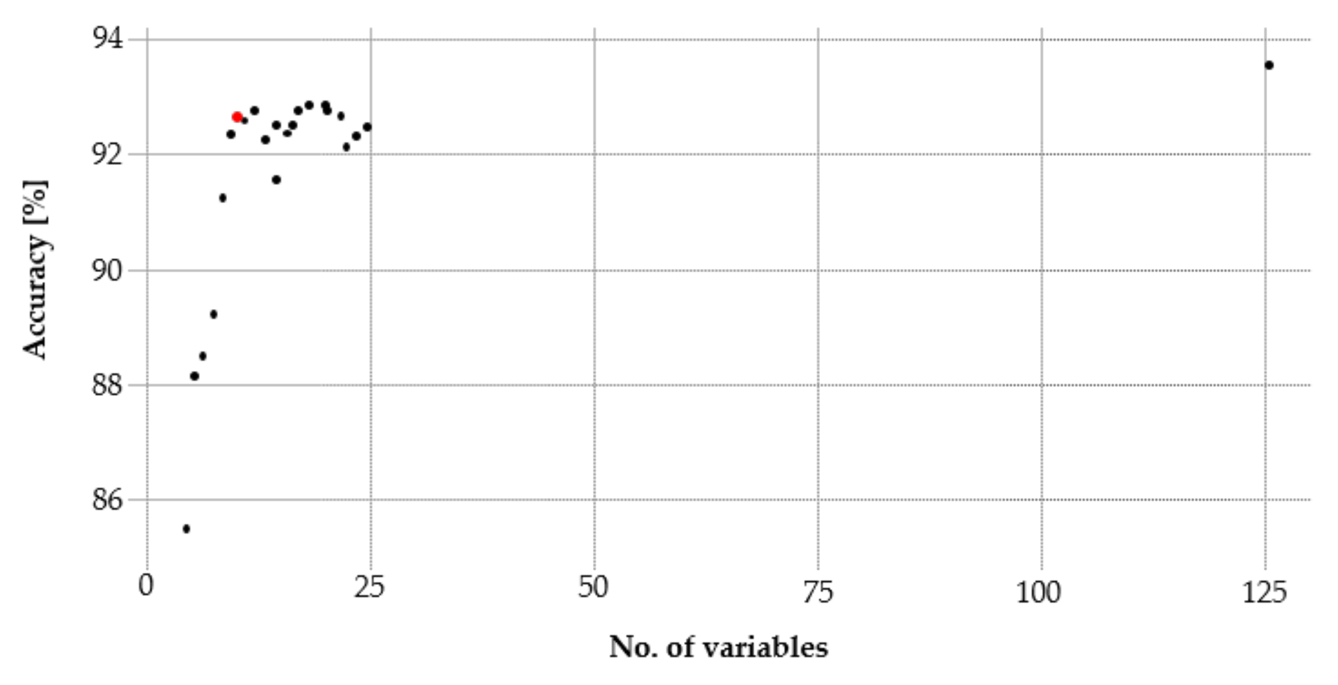
As a result of the training phase, 11 variables with an accuracy of 93% remained. Further variables did not provide a decisive benefit (Figure 4). In addition, the Kappa’s difference of the RF reference model to the RF model using the RFE was significantly smaller (1.7) as compared to the RF model using the VIP (3.6). Accordingly, the 11 variables were applied for the final classification.

Figure 4.
The Recursive Feature Elimination (RFE) identifies a set of 11 variables (red dot) that met the suitable accuracy of 93%.
Also, the user (UA) and producer (PA) accuracies computed with the R package caret [45] confirmed that the performance of these variables resulted in very few misclassifications. The confusion matrix, of all PA and UA proportions, illustrates that only Douglas fir (PM) has low accuracy values due some misidentifications with Norway spruce (PA). All other classes indicate high levels of accuracy (Table 4).

Table 4.
Confusion matrix for all tree classes of the classification key based on reference data; OA: 92.8%.
Concerning the first key question asking which variables were particularly meaningful for differentiation and recognition of a trees’ class, the list of variables selected for the final model provided information on the significance of the individual variables and thus their underlying data sources in accordance with the MDG values (Table 5). Most of the 11 variables were derived from the leaf-off aerial photos, only two came from the leaf-on aerial photos and here the only information derived came from the NDVI. The LiDAR data set contributed one variable to the selection.

Table 5.
List of variables implemented in the final model in descending order of Mean Decrease Gini (MDG) value, Mean Decrease Accuracy (MDA) values are indicated for comparison.
3.2. Recognition of Tree Classes
To answer the second question, which trees classes could be distinguished from each other with high rates of accuracy, the results of the six validation sites were used (Table 6). Based on these independent control sites, it can be stated that deciduous trees such as LD (Larix kaempferii) and DB (deciduous broadleaved species) were well predicted by the model. Picea abies (PA) and snags (WD) were also reliably classified. The classification of Abies alba (AA) was moderately well. Less well identified were Pseudotsuga menziesii (PM) and Pinus sylvestris (PS).

Table 6.
Recognition of tree classes according to Producer’s Accuracy (PA) and User’s Accuracy (UA).
Even though all classes of trees were analyzed, the final classification was deemed best suited for a forest landscape dominated by Norway spruce (Picea abies). This was followed by the next most common species European silver fir (Abies alba) and Scots pine (Pinus sylvestris), i.e., conifers strongly dominate the study area. The remaining classes, Douglas fir (Pseudotsuga menziesii), European larch (Larix decidua including Larix kampferii) and snags occurred in only very small proportions.
According to the accuracy assessment of the final classification, it can be assumed that 89.5% of all tree classes have been recognized correctly. This was estimated using the results of the six validation sites with a total of 505 trees validated by visual interpretation. (Figure 5). Of those 505 trees 53 trees were found misclassified (Table 8). The few misclassifications of Norway spruce could be attributed to their existence on very steep slopes with an eastern exposure and the density of the stands. In these instances, some Norway spruce were classified as European silver fir therefore slightly overrepresenting European silver fir in these locations. In other areas, a surprisingly large number of fir and pine have been classified, although they were not known to occur there in these densities, hence the results of this classification could be subject to a further examination.
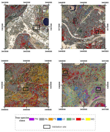
Figure 5.
Result maps of classified tree classes in the four test sites and location of the six validation sites.
Regarding the high overall accuracies (OA: 89.5%), over all studied validation sites with 79 to 90 trees each, confirm the model’s high prediction rate. Three out of the six sites have overall accuracy values >80%, the remaining three have an overall accuracy value >90% (Table 7).

Table 7.
Quality metrics of the accuracy assessment in the six validation sites taking into account the different relief and the occurrence of the tree classes.
At the same time, the balanced accuracy for all samples was more than 90%. In addition, the Cohen’s kappa coefficient () supports the high accuracy of the classification. Whereby, all samples, except sample 2, indicate a near perfect agreement between predicted and verified classes.
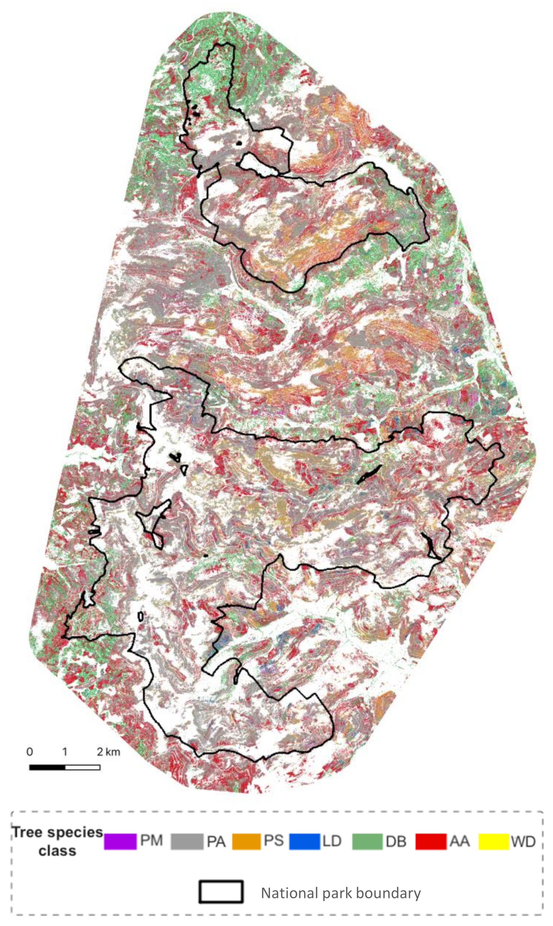
The practical suitability of the approach, which was proven by the test sites, was extended to the entire study area. The resulting tree classes were identified according to the following proportions: 2% Douglas fir (Pseudotsuga menziesii, PM), 59% Norway spruce (Picea abies, PA), 7% Scots pine (Pinus sylvestris, PS), 1% European larch (Larix decidua including Larix kampferii, LD), 8% deciduous broadleaved species (DB were not further differentiated), 22% European silver fir (Abies alba, AA) and 1% snags (WD). The results represent the early years of the BFNP (2014/15) and are a base for long-term monitoring of tree species composition in the area (Figure 6).
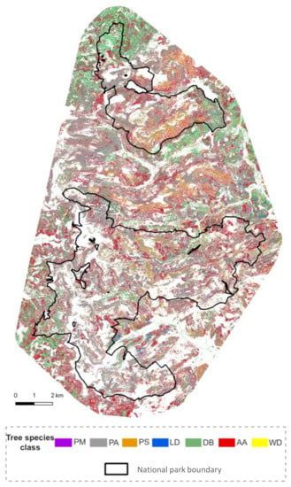
Figure 6.
The classified tree classes as result of the applied classification model for the entire study area.
3.3. Accuracy of Classification
The impact of relief was the most significant impediment to reliable classification. While a good recognition of tree species was produced on level high elevations, on steep and shady slopes the tree classes were often confused (Table 7: site 2). The misclassification of Picea abies (PA), as Abies alba (AA) was mainly due to the impact of relief (Table 8: PA versus AA). However, misclassifications between these species could not be detected on level terrain (Table 7: site 3).

Table 8.
Confusion matrix of the qualitatively validated 505 trees in the six validation sites; OA: 89.5% and Kappa coefficient (): 0.85.
3.4. Importance of Variables
When looking at the variables used to classify the trees a trend can be noted. Variables with spectral information mostly influenced the final classification using the RF algorithm. Apart from these decision variables, the proportion of the LiDAR signal reflected in the upper 150 cm of the cylindrical point cloud to all returns of the cylindrical point cloud played an important role as geometric information, because conical crowns (e.g., Picea abies) could be distinguished from cloud-shaped tree crowns (e.g., deciduous broadleaved species and Pinus sylvestris). Especially because of this variable, the Picea abies (PA) and snags (WD) could be easily separated, but also Pinus sylvestris (PS) and Abies alba (AA) could be well separated from the other classes. The class DB could also be separated although the tree crown shapes varied considerably because in this class several broadleaved species were combined (Figure 7).
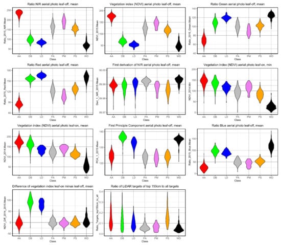
Figure 7.
Violin plots showing the distribution frequencies of classified trees for the 11 variables implemented in the final classification model using the RF algorithm. Metrics of the multispectral data have been calculated from digital numbers and were rescaled to 8-bit range, hence the difference to reflectance-derived NDVI values.
In the final classification model, except of the proportion of the LiDAR signal reflected in the upper 150 cm of the cylindrical point cloud, no other information was included due to low explanatory values. Furthermore, an imbalance was noticed between variables representing spectral properties and those determined from geometric raster data and used in the final model. To sum up, the spectral data derived from the multispectral mosaics were the most important variables in terms of their number and in combination with one important variable derived from the LiDAR data set led to very good classification results.
Additionally, Figure 7 highlights the overriding importance of spectral information when used as decision variables for the classification model. According to the spectral range, the blue wavelength indicates a high importance for the detection of conifers. Particularly the mean NIR ratio, the mean NDVI, the mean green ratio and the mean red ratio, all derived from aerial photos taken during the leaf-off phenophase, provided distinct decision variables. In all cases, the classes AA and WD could be separated from the others particularly well. In addition, species that shed their leaves could be easily distinguished from evergreen species. The leaf-on aerial photos, especially in the form of a vegetation index, are important to classify deciduous species including larch and broad-leaved species, as well as snags. Additionally, the NDVI difference leaf-on minus leaf-off separates deciduous species particularly well from the other classes.
Besides those variables, which resulted in particularly clear classes, the first derivation of the NIR aerial photos from the leaf-off phenophase also contributed remarkably as well as the first derivation of the NIR aerial photos from the leaf-off phenophase. Mathematically, this first derivation is the equivalent to the mean slope to the horizontal and represents the range of reflectance values of biomass. Thus, the lower variability of the PA canopy in general and also compared to other classes in the NIR band derivation resulted in a good differentiation of this species in the corresponding reflectance range. In contrast, the values of the tree classes DB, LD, PM, PS were comparatively far apart in this band. The tree class AA shows an ambiguous trend in the first derivation of the NIR aerial photos in the leaf-off phenophase; as there are both individuals with high and low variance (Figure 7).
4. Discussion
Compared to wall-to-wall mappings that are based on relevant and predefined variables, our study focused on tree species classification without an a priori specified variables. The goal was to find the most helpful variables that could be used for the classification of trees within a large study area, approximately 265 km2. However, a Random Forest approach is usually very data-intensive in the initial training phase and requires as many variables as possible to be tested for their redundancy and potential. Through optimized tuning parameters overfitting is prevented while testing all possible combinations of input data [30]. The ensemble learning approach as part of the applied Random Forest algorithm is the reason why we accepted that some content-relevant variables were rejected as a result of the conducted feature selection techniques. For example a canopy height model was one of many potential variables, but was not selected for the final classification model. Therefore, the applied classification model differs from remotely sensed based forest inventories, where the canopy height model typically plays a major role regardless of the underlying data sources [10,11].
During the training phase, it became clear that the geometric parameters (tree height, slope, curvature and roughness) and topography did not play a major role in the classification. The subordinate role of these variables compared to the spectral data sets was surprising. The imbalance between variables representing spectral properties and those modeling morphometric attributes might be the result of a difference in the pixel resolution, because the pixel resolution was much lower in the relief data. This was detected during ensemble learning. Accordingly, the question remains, what result would even higher resolution data have produced in the classification model? One further explanation for the non-relevance of some geometric variables, could also be that there is no clear, uniform pattern linking relief and tree species in the study area. This could be the subject of a subsequent study in which the tree species will be characterized according to their morphometric properties.
It is also noteworthy that only one of the metrics generated using the airborne laser scanner (LiDAR) was used in the final model (proportion of LiDAR targets of top 150 cm to all targets). No other tree metrics were used for the classification due to their low explanatory power. The selected tree metric importantly helps to describe the shape of the canopy, thus helping to distinguish the rather flat-topped crowns of the Scots pine from the cone-shaped crowns of the fir and spruce [46]. A future study should test whether a selected set of features describing individual tree crowns reach leads to a significantly better classification result as suggested by Torabzadeh et al. [23]. Another reason why no other metric from the LiDAR data was useful in the final classification model could be attributed to geometric structures. They varied as much within the investigated species (intraspecific) as between species (interspecific). Additionally, according to Shi et al. [47] there is a high degree of correlated or redundant information between the metrics of the LiDAR data.
As might be assumed, and as the work of Davison et al. [10] indicates, the leaf-off phase represents the most favorable time for species distinction and it is not likely that further LiDAR surveys during the leaf-on phase would lead to an improvement in data quality [48,49]. But, further improvement of the results would be expected if LiDAR data from the leaf-on and leaf-off phases had been considered in combination [10,47]. The fact that the generated MDG and MDA values of this variable are relatively low compared to the data from the multispectral mosaic (MDG = 18, MDA = 16) can possibly also be attributed to the underlying data preparation or crown segmentation, as is also the case in the studies of Marconi et al. [50].
Generally, the consideration of the phenology and especially the combination of both phenological phases played a major role in the R-G-B-NIR data. This finding also confirms previous evidence in the literature regarding the importance of variables representing phenological phases for airborne data [51] as well as satellite images [52]. Especially, the NDVI differences represent seasonal variations and illustrate the high benefit of multitemporal data in species discrimination. Among others, it is noticeable that the highly correlated variables, e.g., the mean NIR ratio and the mean NVDI based on aerial photos from the leaf-off phenophase were chosen during feature selection. Overall, the reason for the dominance of the leaf-off aerial photos is clearly the strong dynamic within the tree crowns and the better separability of characteristics. However, the available image quality has to be considered as well. As mentioned in the literature [53,54], for the interpretation of our results a more in-depth analysis of the relief is needed in order to clarify the influence of exposition, viewing angle, illumination etc.
We could confirm that Pinus sylvestris (PS) and Picea abies (PA) share similar value ranges regarding relevant variables. The reason for the misclassification of these two most frequently occurring species (PS, PA) is assumed to be the similarity of their range values. Only the ranges of the NIR derivative and the LiDAR proportions differ between them. Thus, the implementation of the NIR derivative can be beneficial for the delineation of PS and PA, because of their different reflectance gradient from the center to the edges of the trees. While PA represents a high gradient in terms of reflectance, PS represents a low gradient due to its mixed reflectance values throughout the canopy. However, further research is needed to confirm the full relevance of both variables. Although an overriding importance of the NIR derivative and the LiDAR proportion could be shown in our study, for a more in depth analysis of the different deciduous species additional texture features should be calculated as recommended by Kuzmin et al. [55].
Additionally, the results highlighted the outstanding importance of spectral information when used as decision variables for the classification model. Also, in the case of the spectral range of the blue wavelength we could confirm a high importance for the detection of conifers, but its role was not as important as was mentioned in the literature [36,56]. Another important variable derived from the spectral signatures marks the first derivation (i.e., the slope) of the NIR band. Following the respective discussion of Fassnacht et al. [3], our study confirms the potential and benefit of specific spectral derivatives.
Nevertheless, an overrepresentation of specific information, due to the inclusion of correlating variables, does not compromise our results since the random combination and arrangement of the training data and features prevented an overfitting of the RF algorithm, as mentioned above [3,30]. Complementary studies, which used more cost-intensive hyperspectral signatures as a data source [15,16,17,18,19,20,57], show that the results of our approach reveal that R-G-B-NIR signatures combined with meaningful LiDAR signals from trees (>15 m height) are promising data sources for achieving highly accurate classification of tree species in a temperate mixed mountain forest landscape.
5. Conclusions
As a training data set, only 11 out of 126 variables were identified as being the most meaningful combination of variables for the studied conifer dominated mountain landscape. These combinations resulted in an accuracy level of 93% whereas other variables did not lead to any significant improvement.
Most of the 11 variables were derived from the leaf-off aerial photos, only two came from the leaf-on aerial photos and here the attributes were linked to NDVI; the LiDAR data set contributed only one variable. We attributed the great importance of the R-G-B-NIR signatures and vegetation indices opposite the geometric parameters to the comparatively high spatial resolution of the spectral datasets. In particular, it has been shown that the blue wavelength is of overriding importance in delineating conifers. We can explain the dominance of the leaf-off aerial photos with the dynamic reflectance values within the tree crowns. As was to be expected, the NDVI difference of leaf-on and leaf-off separates deciduous species and the other species very well. The only LiDAR variable we implemented was important to describe the shape of the canopy, which distinguished the rather flat-topped Scots pine from the cone-shaped canopies of fir and spruce.
With respect to the classification quality, we elaborated that the implemented approach predicted deciduous trees (LD and DB) very well, also species of the class Picea abies (PA) and snags (WD) were reliably classified by the model, Abies alba (AA) was moderately well recognized, whereas Pseudotsuga menziesii (PM) and Pinus sylvestris were the least well identified. Finally, the high overall accuracies (OA: 89.5%), achieved on all validation sites studied, with 79 to 90 trees each, confirm the model’s high prediction rate.
Using this approach, the Random Forest algorithm applied with the small set of 11 variables was shown to be able to classify individual tree species in a temperate mixed mountain forest landscape with a high degree of accuracy. Consequently, this underlines the practical suitability of our approach for monitoring protected areas as proven by the classification of the complete study area of 256km2. Thus, the approach we presented can substantially increase the efficiency of traditional tree species monitoring methods in temperate mixed forests. Especially, in comparison to commonly used methods of forest inventory, our approach provides not only a static picture of the tree species composition distribution, but also provides an exact recognition of tree classes on an individual tree level, so that ecological process monitoring can be conducted. Also, in contrast to studies that concentrate on more cost-intensive hyperspectral aerial images, this work shows that the complementary application of multispectral aerial photos and LiDAR data can deliver high quality classifications. However, in order to generate even higher accuracies on very steep terrain, more research with higher spatial resolution of morphometric parameters is needed. It seems also to be meaningful to test the methodology presented on an unknown Central European forest landscape with equivalent tree classes in a wall-to-wall approach to better understand its transferability.
Supplementary Materials
The following are available at https://www.mdpi.com/article/10.3390/rs13224657/s1. We provide the R source code for training phase and classification as supplementary html-markdown file.
Author Contributions
(In alphabetical order) conceptualization: C.D., S.G., R.H. and K.S.; methodology: C.D., R.H. and K.S.; software: C.D. and K.S.; validation: K.S.; formal analysis: K.S.; investigation, K.S.; resources: C.D.; data curation: C.D. and K.S.; writing—original draft preparation: C.D., S.G., R.H. and K.S.; writing, review and editing: C.D., S.G., R.H. and K.S.; visualization: C.D. and K.S. All authors have read and agreed to the published version of the manuscript.
Funding
The article processing charge was funded by the Baden-Wuerttemberg State Ministry of Science, Research and Art and the University of Freiburg in the funding programme Open Access Publishing.
Acknowledgments
The authors are grateful for the support from the Black Forest National Park administration specifically from Sönke Birk and Marc Förschler. The authors would like to thank Bernhard Thiel for the improvement of the English. We would also like to show our gratitude to the editor and the anonymous reviewers for their insights and recommendations.
Conflicts of Interest
The authors declare no conflict of interest. The funders had no role in the design of the study; in the collection, analyses, or interpretation of data; in the writing of the manuscript, or in the decision to publish the results.
Abbreviations
The following abbreviations are used in this manuscript:
| AA | Abies alba (European silver fir) |
| ASCII | American Standard Code for Information Interchange |
| B | Blue |
| BFNP | Black Forest National Park |
| BW | Baden-Württemberg |
| C | Celsius |
| CHM | Canopy Height Model |
| DB | deciduous broadleaved species |
| DSM | Digital Surface Model |
| DTM | Digital Terrain Model |
| et al. | et alia (and others) |
| EVI | Enhanced Vegetation Index |
| G | Green |
| GDAL | Geospatial Data Abstraction Library |
| i.e. | id est (that is) |
| IR | Infrared |
| IUCN | International Union for Conservation of Nature |
| km | kilometer |
| LD | Larix kampferii (European Larch) |
| LiDAR | Light Detection and Ranging |
| m | meter |
| max | maximum |
| MDA | Mean decrease in accuracy |
| MDG | Mean decrease in Gini |
| min | minimum |
| Mio. | million |
| mm/a | millimeter per year |
| mtry | number of selected features used for each decision tree |
| NDVI | Normalized Difference Vegetation Index |
| NIR | Near Infrared |
| ntree | number of trees |
| OA | Overall Accuracy |
| OOB (error) | out of the box (error) |
| PA | Picea abies (Norway spruce) |
| PA | Producer’s accuracy |
| PCA | Principal Component Analysis |
| PM | Pseudotsuga menziesii (Douglas fir) |
| PS | Pinus sylvestris (Scots pine) |
| R | Red |
| RAM | Random Access Memory |
| RF | Random Forest |
| RFE | Recursive Feature Elimination |
| s. | see |
| sd | standard deviation |
| TDOP | True Digital Orthophoto |
| UA | User’s accuracy |
| UAV | Unmanned Aerial Vehicle |
| VIP | Variable Importance Plot |
| WD | standing coarse woody debris (used standing dead or snag) |
References
- Latifi, H.; Heurich, M. Multi-scale remote sensing-assisted forest inventory: A glimpse of the state-of-the-art and future prospects. Remote Sens. 2019, 11, 1260. [Google Scholar] [CrossRef] [Green Version]
- Waser, L.T.; Straub, C. Baumartenerkennung mit optischen Fernerkundungsdaten-Stand und Perspektiven. Forstl. Forschungsberichte MüNchen 2015, 214, 65–75. [Google Scholar]
- Fassnacht, F.E.; Latifi, H.; Stereńczak, K.; Modzelewska, A.; Lefsky, M.; Waser, L.T.; Straub, C.; Ghosh, A. Review of studies on tree species classification from remotely sensed data. Remote Sens. Environ. 2016, 186, 64–87. [Google Scholar] [CrossRef]
- Stolton, S.; Shadie, P.; Dudley, N. IUCN WCPA Best Practice Guidance on Recognising Protected Areas and Assigning Management Categories and Governance Types. In Guidelines for Applying Protected Area Management Categories; Dudley, N., Ed.; IUCN: Gland, Switzerland, 2008; p. 86. [Google Scholar]
- Pickett, S.T.; White, P.S. The Ecology of Natural Disturbance and Patch Dynamics, 1st ed.; Academic Press: San Diego, CA, USA, 1985. [Google Scholar]
- Fischer, A.; Marshall, P.; Camp, A. Disturbances in deciduous temperate forest ecosystems of the northern hemisphere: Their effects on both recent and future forest development. Biodivers. Conserv. 2013, 22, 1863–1893. [Google Scholar] [CrossRef]
- Schelhaas, M.J.; Nabuurs, G.J.; Schuck, A. Natural disturbances in the European forests in the 19th and 20th centuries. Glob. Chang. Biol. 2003, 9, 1620–1633. [Google Scholar] [CrossRef]
- Hasel, K. Forstgeschichte: Ein Grundriss für Studium und Praxis; Parey: Hamburg, Germany, 1985; Volume 48. [Google Scholar]
- White, J.C.; Coops, N.C.; Wulder, M.A.; Vastaranta, M.; Hilker, T.; Tompalski, P. Remote Sensing Technologies for Enhancing Forest Inventories: A Review. Can. J. Remote Sens. 2016, 42, 619–641. [Google Scholar] [CrossRef] [Green Version]
- Davison, S.; Donoghue, D.N.; Galiatsatos, N. The effect of leaf-on and leaf-off forest canopy conditions on LiDAR derived estimations of forest structural diversity. Int. J. Appl. Earth Obs. Geoinf. 2020, 92, 102160. [Google Scholar] [CrossRef]
- Michez, A.; Huylenbroeck, L.; Bolyn, C.; Latte, N.; Bauwens, S.; Lejeune, P. Can regional aerial images from orthophoto surveys produce high quality photogrammetric Canopy Height Model? A single tree approach in Western Europe. Int. J. Appl. Earth Obs. Geoinf. 2020, 92, 102190. [Google Scholar] [CrossRef]
- Gara, T.W.; Darvishzadeh, R.; Skidmore, A.K.; Wang, T.; Heurich, M. Accurate modelling of canopy traits from seasonal Sentinel-2 imagery based on the vertical distribution of leaf traits. ISPRS J. Photogramm. Remote Sens. 2019, 157, 108–123. [Google Scholar] [CrossRef]
- Engler, R.; Waser, L.T.; Zimmermann, N.E.; Schaub, M.; Berdos, S.; Ginzler, C.; Psomas, A. Combining ensemble modeling and remote sensing for mapping individual tree species at high spatial resolution. For. Ecol. Manag. 2013, 310, 64–73. [Google Scholar] [CrossRef]
- He, Y.; Yang, J.; Caspersen, J.; Jones, T. An operational workflow of deciduous-dominated forest species classification: Crown delineation, gap elimination, and object-based classification. Remote Sens. 2019, 11, 2078. [Google Scholar] [CrossRef] [Green Version]
- Modzelewska, A.; Fassnacht, F.E.; Stereńczak, K. Tree species identification within an extensive forest area with diverse management regimes using airborne hyperspectral data. Int. J. Appl. Earth Obs. Geoinf. 2020, 84, 101960. [Google Scholar] [CrossRef]
- Ballanti, L.; Blesius, L.; Hines, E.; Kruse, B. Tree species classification using hyperspectral imagery: A comparison of two classifiers. Remote Sens. 2016, 8, 445. [Google Scholar] [CrossRef] [Green Version]
- Fricker, G.A.; Ventura, J.D.; Wolf, J.A.; North, M.P.; Davis, F.W.; Franklin, J. A convolutional neural network classifier identifies tree species in mixed-conifer forest from hyperspectral imagery. Remote Sens. 2019, 11, 2326. [Google Scholar] [CrossRef] [Green Version]
- Trier, Ø.D.; Salberg, A.B.; Kermit, M.; Rudjord, Ø.; Gobakken, T.; Næsset, E.; Aarsten, D. Tree species classification in Norway from airborne hyperspectral and airborne laser scanning data. Eur. J. Remote Sens. 2018, 51, 336–351. [Google Scholar] [CrossRef]
- Dalponte, M.; Frizzera, L.; Gianelle, D. Individual tree crown delineation and tree species classification with hyperspectral and LiDAR data. PeerJ 2019, 6, e6227. [Google Scholar] [CrossRef] [PubMed]
- Maschler, J.; Atzberger, C.; Immitzer, M. Individual tree crown segmentation and classification of 13 tree species using Airborne hyperspectral data. Remote Sens. 2018, 10, 1218. [Google Scholar] [CrossRef] [Green Version]
- Hartling, S.; Sagan, V.; Sidike, P.; Maimaitijiang, M.; Carron, J. Urban tree species classification using a worldview-2/3 and liDAR data fusion approach and deep learning. Sensors 2019, 19, 1284. [Google Scholar] [CrossRef] [PubMed] [Green Version]
- Shi, Y.; Wang, T.; Skidmore, A.K.; Heurich, M. Improving LiDAR-based tree species mapping in Central European mixed forests using multi-temporal digital aerial colour-infrared photographs. Int. J. Appl. Earth Obs. Geoinf. 2020, 84, 101970. [Google Scholar] [CrossRef]
- Torabzadeh, H.; Leiterer, R.; Hueni, A.; Schaepman, M.E.; Morsdorf, F. Tree species classification in a temperate mixed forest using a combination of imaging spectroscopy and airborne laser scanning. Agric. For. Meteorol. 2019, 279, 107744. [Google Scholar] [CrossRef]
- Heinzel, J.; Koch, B. Exploring full-waveform LiDAR parameters for tree species classification. Int. J. Appl. Earth Obs. Geoinf. 2011, 13, 152–160. [Google Scholar] [CrossRef]
- Mountrakis, G.; Im, J.; Ogole, C. Support vector machines in remote sensing: A review. ISPRS J. Photogramm. Remote Sens. 2011, 66, 247–259. [Google Scholar] [CrossRef]
- Tuia, D.; Volpi, M.; Copa, L.; Kanevski, M.; Muñoz-Marí, J. A survey of active learning algorithms for supervised remote sensing image classification. IEEE J. Sel. Top. Signal Process. 2011, 5, 606–617. [Google Scholar] [CrossRef]
- Cutler, A.; Cutler, D.R.; Stevens, J.R. Ensemble Machine Learning. Ensemble Machine Learning; Springer Nature: Cham, Switzerland, 2012. [Google Scholar] [CrossRef]
- Ma, L.; Liu, Y.; Zhang, X.; Ye, Y.; Yin, G.; Johnson, B.A. Deep learning in remote sensing applications: A meta-analysis and review. ISPRS J. Photogramm. Remote Sens. 2019, 152, 166–177. [Google Scholar] [CrossRef]
- Natesan, S.; Armenakis, C.; Vepakomma, U. Resnet-based tree species classification using uav images. ISPRS Arch. 2019, 42, 475–481. [Google Scholar] [CrossRef] [Green Version]
- Breiman, L. Random forests. Mach. Learn. 2001, 45, 5–32. [Google Scholar] [CrossRef] [Green Version]
- Liaw, A.; Wiener, M. Classification and Regression by randomForest. R News 2002, 2, 18–22. [Google Scholar]
- Pal, M. Random forest classifier for remote sensing classification. Int. J. Remote Sens. 2005, 26, 217–222. [Google Scholar] [CrossRef]
- Lawrence, R.L.; Wood, S.D.; Sheley, R.L. Mapping invasive plants using hyperspectral imagery and Breiman Cutler classifications (randomForest). Remote Sens. Environ. 2006, 100, 356–362. [Google Scholar] [CrossRef]
- Belgiu, M.; Drăgu, L. Random forest in remote sensing: A review of applications and future directions. ISPRS J. Photogramm. Remote Sens. 2016, 114, 24–31. [Google Scholar] [CrossRef]
- Georganos, S.; Grippa, T.; Niang Gadiaga, A.; Linard, C.; Lennert, M.; Vanhuysse, S.; Mboga, N.; Wolff, E.; Kalogirou, S. Geographical random forests: A spatial extension of the random forest algorithm to address spatial heterogeneity in remote sensing and population modelling. Geocarto Int. 2019, 36, 121–136. [Google Scholar] [CrossRef] [Green Version]
- Immitzer, M.; Atzberger, C.; Koukal, T. Tree species classification with Random forest using very high spatial resolution 8-band worldView-2 satellite data. Remote Sens. 2012, 4, 2661–2693. [Google Scholar] [CrossRef] [Green Version]
- LGRB. Geologische Karte von Baden-Württemberg 1:50.000 (GeoLa); Landesamt für Geologie, Rohstoffe und Bergbau: Freiburg, Germany, 2021. [Google Scholar]
- LGRB. Bodenkarte von Baden-Württemberg 1:50,000 (GeoLa); Landesamt für Geologie, Rohstoffe und Bergbau: Freiburg, Germany, 2021. [Google Scholar]
- Schultz, J. Die Ökozonen der Erde; Ulmer: Stuttgart, Germany, 2016. [Google Scholar]
- WaBoA. Wasser-und Bodenatlas Baden-Württemberg; Landesanstalt für Umwelt, Messungen und Naturschutz Baden-Württemberg: Karlsruhe, Germany, 2007. [Google Scholar]
- Weinacker, H.; Koch, B.; Weinacker, R. TreesVis—A software system for simultaneous 3D-real-time visualisation of DTM, DSM, laser raw data, multispectral data, simple tree and building models. Int. Arch. Photogramm. Remote Sens. Spat. Inf. Sci. 2004, 36, 90–95. [Google Scholar]
- O’Hara, K.; Latham, P.A.; Hessburg, P.; Bradley, S.G. A Structural Classification for Inland Northwest Forest Vegetation. West. J. Appl. For. 1996, 11, 97–102. [Google Scholar] [CrossRef] [Green Version]
- Falkowski, M.J.; Evans, J.S.; Martinuzzi, S.; Gessler, P.E.; Hudak, A.T. Characterizing forest succession with lidar data: An evaluation for the Inland Northwest, USA. Remote Sens. Environ. 2009, 113, 946–956. [Google Scholar] [CrossRef] [Green Version]
- GDAL/OGR Contributors. GDAL/OGR Geospatial Data Abstraction Software Library; Open Source Geospatial Foundation: Beaverton, OR, USA, 2021. [Google Scholar]
- Kuhn, M. Building Predictive Models in R Using the caret Package. J. Stat. Softw. 2008, 28, 1–26. [Google Scholar] [CrossRef] [Green Version]
- Holmgren, J.; Persson, Å.; Söderman, U. Species identification of individual trees by combining high resolution LiDAR data with multi-spectral images. Int. J. Remote Sens. 2008, 29, 1537–1552. [Google Scholar] [CrossRef]
- Shi, Y.; Wang, T.; Skidmore, A.K.; Heurich, M. Important LiDAR metrics for discriminating forest tree species in Central Europe. ISPRS J. Photogramm. Remote Sens. 2018, 137, 163–174. [Google Scholar] [CrossRef]
- Kim, S.; McGaughey, R.J.; Andersen, H.E.; Schreuder, G. Tree species differentiation using intensity data derived from leaf-on and leaf-off airborne laser scanner data. Remote Sens. Environ. 2009, 113, 1575–1586. [Google Scholar] [CrossRef]
- Reitberger, J.; Krzystek, P.; Stilla, U. Analysis of full waveform LIDAR data for the classification of deciduous and coniferous trees. Int. J. Remote Sens. 2008, 29, 1407–1431. [Google Scholar] [CrossRef]
- Marconi, S.; Graves, S.J.; Gong, D.; Nia, M.S.; Le Bras, M.; Dorr, B.J.; Fontana, P.; Gearhart, J.; Greenberg, C.; Harris, D.J.; et al. A data science challenge for converting airborne remote sensing data into ecological information. PeerJ 2019, 6, e5843. [Google Scholar] [CrossRef] [Green Version]
- Hill, R.A.; Wilson, A.K.; George, M.; Hinsley, S.A. Mapping tree species in temperate deciduous woodland using time-series multi-spectral data. Appl. Veg. Sci. 2010, 13, 86–99. [Google Scholar] [CrossRef]
- Persson, M.; Lindberg, E.; Reese, H. Tree species classification with multi-temporal Sentinel-2 data. Remote Sens. 2018, 10, 1794. [Google Scholar] [CrossRef] [Green Version]
- Rautiainen, M.; Lukeš, P.; Homolová, L.; Hovi, A.; Pisek, J.; Mõttus, M. Spectral properties of coniferous forests: A review of in situ and laboratory measurements. Remote Sens. 2018, 10, 207. [Google Scholar] [CrossRef] [Green Version]
- Lukeš, P.; Stenberg, P.; Rautiainen, M.; Mõttus, M.; Vanhatalo, K.M. Optical properties of leaves and needles for boreal tree species in Europe. Remote Sens. Lett. 2013, 4, 667–676. [Google Scholar] [CrossRef]
- Kuzmin, A.; Korhonen, L.; Manninen, T.; Maltamo, M. Automatic segment-level tree species recognition using high resolution aerial winter imagery. Eur. J. Remote Sens. 2016, 49, 239–259. [Google Scholar] [CrossRef]
- Waser, L.T.; Ginzler, C.; Kuechler, M.; Baltsavias, E.; Hurni, L. Semi-automatic classification of tree species in different forest ecosystems by spectral and geometric variables derived from Airborne Digital Sensor (ADS40) and RC30 data. Remote Sens. Environ. 2011, 115, 76–85. [Google Scholar] [CrossRef]
- Marrs, J.; Ni-Meister, W. Machine learning techniques for tree species classification using co-registered LiDAR and hyperspectral data. Remote Sens. 2019, 11, 819. [Google Scholar] [CrossRef] [Green Version]
Publisher’s Note: MDPI stays neutral with regard to jurisdictional claims in published maps and institutional affiliations. |
© 2021 by the authors. Licensee MDPI, Basel, Switzerland. This article is an open access article distributed under the terms and conditions of the Creative Commons Attribution (CC BY) license (https://creativecommons.org/licenses/by/4.0/).


