Article

UAV-Assisted Thermal Infrared and Multispectral Imaging of Weed Canopies for Glyphosate Resistance Detection

1
Department of Agriculture and Biosystems Engineering, North Dakota State University, Fargo, ND 58108-6050, USA
2
NDSU Carrington Research Extension Center, Carrington, ND 58421-0219, USA
3
Department of Plant Sciences, North Dakota State University, Fargo, ND 58108-6050, USA
*
Author to whom correspondence should be addressed.
Remote Sens. 2021, 13(22), 4606; https://doi.org/10.3390/rs13224606
Submission received: 18 September 2021 / Revised: 6 November 2021 / Accepted: 13 November 2021 / Published: 16 November 2021
(This article belongs to the Special Issue UAV Imagery for Precision Agriculture)

Abstract

:
The foundation of contemporary weed management practices in many parts of the world is glyphosate. However, dependency on the effectiveness of herbicide practices has led to overuse through continuous growth of crops resistant to a single mode of action. In order to provide a cost-effective weed management strategy that does not promote glyphosate-resistant weed biotypes, differences between resistant and susceptible biotypes have to be identified accurately in the field conditions. Unmanned Aerial Vehicle (UAV)-assisted thermal and multispectral remote sensing has potential for detecting biophysical characteristics of weed biotypes during the growing season, which includes distinguishing glyphosate-susceptible and glyphosate-resistant weed populations based on canopy temperature and deep learning driven weed identification algorithms. The objective of this study was to identify herbicide resistance after glyphosate application in true field conditions by analyzing the UAV-acquired thermal and multispectral response of kochia, waterhemp, redroot pigweed, and common ragweed. The data were processed in ArcGIS for raster classification as well as spectral comparison of glyphosate-resistant and glyphosate-susceptible weeds. The classification accuracy between the sensors and classification methods of maximum likelihood, random trees, and Support Vector Machine (SVM) were compared. The random trees classifier performed the best at 4 days after application (DAA) for kochia with 62.9% accuracy. The maximum likelihood classifier provided the highest performing result out of all classification methods with an accuracy of 75.2%. A commendable classification was made at 8 DAA where the random trees classifier attained an accuracy of 87.2%. However, thermal reflectance measurements as a predictor for glyphosate resistance within weed populations in field condition was unreliable due to its susceptibility to environmental conditions. Normalized Difference Vegetation Index (NDVI) and a composite reflectance of 842 nm, 705 nm, and 740 nm wavelength managed to provide better classification results than thermal in most cases.

1. Introduction

Herbicide usage provides crop producers with multiple benefits, including increased crop yield, timely and affordable management, reduced weed pressure, and reduction in soil structure degradation caused by conventional tillage methods [1,2,3]. Scientific advancements in the 1990s supported the development of a transgenic herbicide-resistant soybean varieties that allowed crop producers to spray broad-spectrum herbicides to kill weeds with no concern of harming their crops [4]. However, dependency on the effectiveness of herbicide applications has led to overuse through continuous growth of herbicide-resistant crops and the application of the associated weed control agent [5]. In 2010, 93% of all soybeans grown in the USA were herbicide-resistant, as were 78% of all cotton and 70% of all maize varieties [6]. This overuse has caused genetic shifts in weed populations resulting in the success of resistant biotypes [7,8]. Studies estimate that herbicide-resistant management (HRM) has increased herbicide costs in states such as Iowa by $20–40 per acre from 2013–2017 [9].
Glyphosate (N-phosphonomethyl-glycine) is one of the most common herbicides in production agriculture [10]. Developed in 1974, glyphosate is a non-selective herbicide that inhibits the enzyme enolpyruvyl shikimate-3-phosphate synthase (EPSPS) from developing amino acids required for protein synthesis [11]. Additional symptoms of glyphosate application include photosynthetic rate reduction, inhibition of growth, and chlorosis of plant tissue [12]. The highly effective herbicide quickly established widespread use by crop producers, accelerating the evolution of resistance mechanisms within weeds [13]. Moderate resistance is achieved in some weeds by mutations that occur at the targeted enzyme. However, in some species the translocation of glyphosate through the non-targeted parts of the plants (i.e., plant leaves) reduces the herbicide’s ability to reach the root and apical meristems where the inhibition of EPSPS can occur [6].
Distinguishing susceptible and resistant populations of weeds is a challenging task. Prior to herbicide application, there is no significant difference in the visual appearance of resistant and susceptible weeds of the same species that can be noted during scouting [14]. Hyperspectral systems to detect differences between resistant and susceptible biotypes show potential in controlled environments, but their effectiveness is drastically reduced once introduced to field conditions [15]. Lab testing for an accumulation of shikimic acid within plant leaves is one method used to identify glyphosate resistance, but its lack of practicality does not justify its use in large scale applications [16]. The development of a method that can indicate herbicide resistance within an acceptable timeframe after application has great potential to help growers manage their fields more effectively [17].
Researchers at North Dakota State University (NDSU) pursued an alternative method of herbicide resistance detection that utilized thermal imaging technology [18]. Thermal imaging has shown potential in detecting plant canopies that are experiencing increased levels of stress and reduced rates of photosynthesis [19]. The application of glyphosate to susceptible plants causes a reduced photosynthetic rate due the inhibition of stomatal conductance [20]. The reduction in stomatal activity lowers the ability for transpiration of water to be performed within the plant leaf, therefore resulting in increased leaf temperature [21]. The study hypothesized glyphosate-susceptible plant canopies would emit a significantly higher temperature than resistant canopies and that the temperature differences could be recorded using a thermal imager. It was reported that glyphosate-susceptible populations of ragweed, waterhemp, and kochia had higher canopy temperatures in comparison to resistant populations after glyphosate [22]. The canopy temperature values were then used to train a support vector machine (SVM) classifier that could identify the weeds that exhibited glyphosate resistance with accuracies exceeding 90% for all three species [18].
Subsequent greenhouse studies were performed with the objective of validating the hypothesis that glyphosate-resistant weeds can be identified using thermal imagery [18]. In these studies, glyphosate was applied to populations of waterhemp, kochia, common ragweed, and redroot pigweed and monitored with hourly image captures from a thermal camera [22]. The weeds selected were determined to be most relevant to North Dakota agriculture and showed the most potential for glyphosate resistance [23,24,25]. The SVM classification strategy was once again utilized to validate the original findings as well as one tailed t-testing to investigate if glyphosate-susceptible weeds consistently maintained higher canopy temperatures than glyphosate-resistant weeds.
Analogous to thermal sensing, multispectral sensing is also used extensively within agriculture [26,27,28]. Multispectral sensing is the practice of using one sensor to image multiple areas of the light spectrum at the same time [29]. When paired with Unmanned Aerial Vehicle (UAV), multispectral sensing payloads have proven to be powerful detectors of biophysical characteristics of vegetation during the growing season [30]. Multispectral cameras capture image data within specified wavelengths of the electromagnetic spectrum, most commonly in the blue, green, red, red-edge, and near-infrared (NIR) wavelengths. However, some sensors such as the Micasense Red-Edge MX Dual Camera are capable of capturing up to ten different wavelengths including visible and non-visible, instantaneously [31].
The high spatial and spectral resolution provided by UAV-assisted multispectral cameras can be used for a variety of agricultural applications including high-throughput phenotyping, disease identification and severity analysis, nutrient management, and weed identification and mapping [32,33]. Rapid identification of plant height, canopy cover, vegetation index, and flowering stage was performed in cotton fields to enhance breeding using multispectral images over multiple stages of the growing season [34]. Potato late blight disease severity was measured using leaf and canopy measurements from the red and red-edge wavelengths with classification accuracies as high as 89.33% [35]. Optimal, site specific, nitrogen fertilizer rate was investigated by Thompson and Puntl. Their use of multispectral sensors reduced nitrogen application rates by approximately 31 kg N ha−1 without causing yield losses and improved nitrogen use efficiency by as much as 18% [36]. Finally, computational deep learning with multispectral images provided a practical solution to identifying weeds in a sugarbeet field by detecting subtle differences in shapes and reflectance patterns of their leaf canopies [37].
The introduction of newer, higher resolution thermal imaging systems that are compatible with UAVs have boosted the practical use of thermography in agriculture [38,39,40,41]. UAV thermal remote sensing applications include monitoring plant water stress, detection of diseases, and plant phenotyping [42,43,44]. It was reported that UAV thermal sensing could also offer remote sensing data for orchard management including water management by observing the fruit-tree canopy temperature variations [45,46,47]. Remote thermal sensing could enable real-time site-specific management techniques such as crop and weed identification, yield prediction, and crop stress assessment when combined with machine learning [46,48]. Thermal measurement as complementary to other sensor measurements such as hyperspectral, visible, and optical distance has also proved to be more effective on field scale crop phenotyping [49,50,51]. In example, complementary sugar beet canopy temperature measurements with UAV infrared and Red, Green, and Blue (RGB) measurements were proved to improve the accuracy of UAV thermal measurements at altitudes below 40 m [52]. Another direct use of UAV thermal remote sensing can be given as nitrogen fertilization management with spatial clustering models [53,54]. Most of these applications are used to monitor crops, and the investigation of other types of vegetation within agricultural systems is needed. Weed control is a critical component in large-scale farming and the unexplored potential of thermal imagery using UAVs could boost the capabilities of site-specific weed management technology [55]. Therefore, the UAV-assisted thermal imagery could be used as a practical solution to identify glyphosate-susceptible and glyphosate-resistant weed populations based on canopy temperature. Particularly, the study in this paper extends the work previously accomplished in greenhouse environment to a field evaluation [22].
The objective of this study was to identify herbicide resistance after glyphosate application in true field conditions by analyzing the thermal and multispectral response of weed species of waterhemp (Amaranthus rudis), kochia (Kochia scoparia), common ragweed (Ambrosia artemisiifolia), and redroot pigweed (Amaranthus retroflexus).

2. Materials and Methods

2.1. Experiment Site and Data Collection

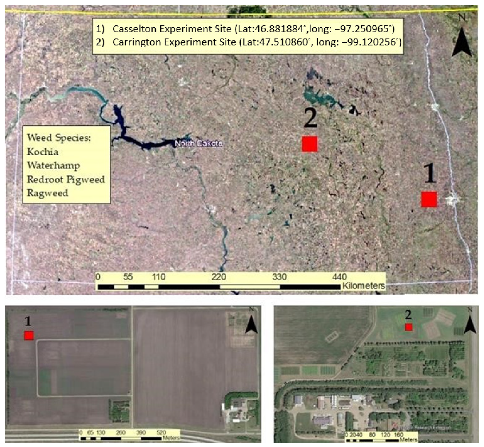
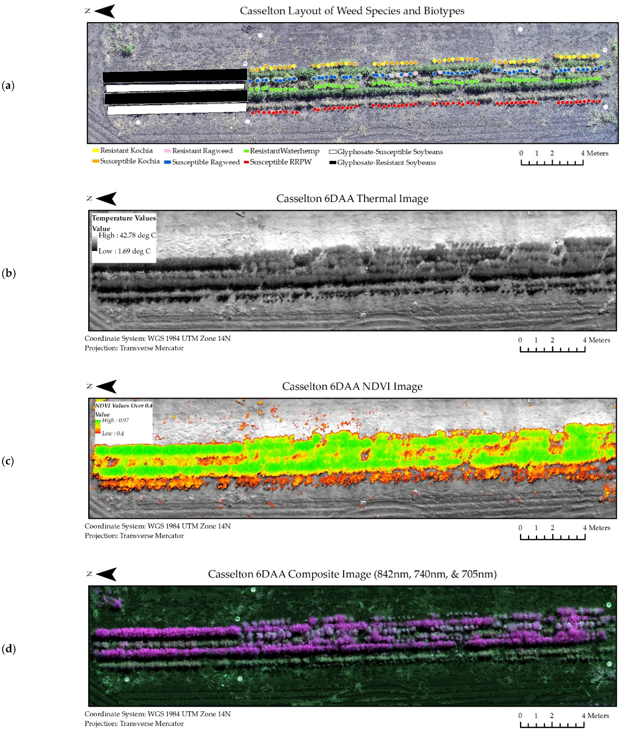
The experiment was conducted at two locations. One location was the NDSU Agronomy Seed Farm in Casselton, ND, USA while the other was conducted at the NDSU Research and Extension Center in Carrington, ND, USA (Figure 1). Each location contained a plot measuring approximately 33 m in length and 3.5 m in width (115 m2). Data collections were performed from the middle to end of August 2020 while all the plants were in vegetative growth stage. At the Casselton location, a combination of Roundup Ready 2 Xtend and ND Stutsman conventional soybean was planted in alternating fashion in 4 rows with 76 cm (30 inch) row spacing. A center-pivot irrigation system was not available at this site, so water was provided to the weed plants using a truck-mounted water tank.
At this location, the soil series was predominantly Kindred-Bearden silty clay loams that are somewhat poorly drained and nonsaline [56]. Buckets of soil were collected at the location and brought to the Agricultural Experiment Station Greenhouse at the NDSU campus in Fargo, ND to be autoclaved. Once the autoclave process was complete, the soil was used to germinate the weed populations in greenhouse conditions at another location on campus. The soil was distributed into 9 cm square pots with 13 cm height and weed seeds were placed at approximately 3 cm soil depth. A total of 60 kochia plants, 60 waterhemp plants, 60 redroot pigweed plants, and 30 ragweed plants were successfully grown and transplanted to the field (Figure 1). To increase plant population, a selection of naturally occurring ragweed plants was transplanted from site location and introduced to the plot, resulting in a total number of 59 ragweed plants. The weed populations were comprised equally of two different biotypes, one being selected for glyphosate resistance and the other for glyphosate susceptibility. Glyphosate-susceptible waterhemp was not available when the experiment was conducted, so redroot pigweed was used as a surrogate. Plants were organized in a randomized complete block design based on their believed resistance status and planted in between the soybean rows with one species occupying a single row at a time. When the weeds were approximately 12–15 cm tall, 2 L/ha of Roundup Powermax (48.7% glyphosate) with Class Act NG at 2% v/v was applied to induce symptomology on the susceptible biotypes.
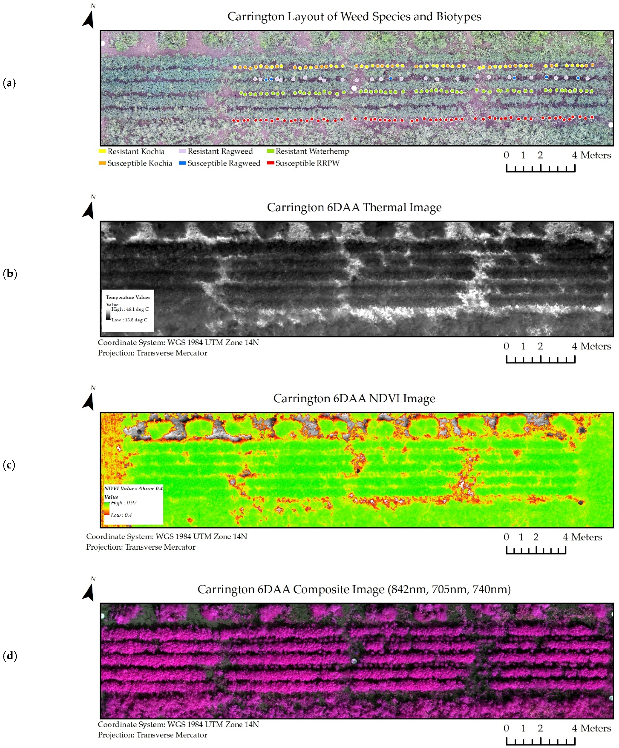
At the Carrington location, five rows of Roundup Ready 2 Xtend (Bayer, Whippany, NJ, USA) Soybeans (Glycine Max) were planted with 76 cm row spacing. A center pivot irrigation system at this location was utilized to provide a constant water source for the plot. The soil series present at this location is predominantly Heimdal-Emrick (G229B) loams which are well drained and slightly saline [57]. Buckets of soil were also collected at this location and brought to the Agricultural Experiment Station Greenhouse at NDSU in Fargo, ND to be autoclaved. The soil was then returned to a greenhouse located at the Carrington location where weed populations were grown in 8 cm diameter pots. A total of 60 kochia plants, 60 waterhemp plants, 60 redroot pigweed plants, and 30 ragweed plants were successfully grown and then transplanted to the field plot in randomized fashion. When the weeds were approximately 12–15 cm tall, 2 L/ha of Roundup Powermax (48.7% glyphosate) with Class Act NG at 2% v/v was applied to induce symptomology on the susceptible biotypes.

2.2. UAV Equipment and Flight Parameters

Image data collection from the experiment sites was performed using a Zenmuse XT2 RGB/Thermal camera (DJI Technology Co., Ltd., Shenzhen, China) and a Micasense Red-Edge MX Dual camera System (Micasense, Seattle, WA, USA). The Zenmuse XT2 provided both RGB and thermal image data, but only the thermal image data were used for testing. The Red-Edge MX Dual camera system provided ten bands of spectral data. Imagers on the dual camera provided a selection of imagery around the blue, green, red, red-edge, and NIR wavelengths. Both systems were mounted simultaneously on a DJI M600 Pro UAV (DJI Technology Co., Ltd., Shenzhen, China).
Due to restrictions with the flight planning software, simultaneous image capture for both systems could not be performed at an altitude less than 25 m. In addition, the Zenmuse XT2 had lower pixel resolution than the Red-Edge MX Dual camera requiring lower altitude flights for thermal image collection for proper image processing. Therefore, an 8 m manual flight was conducted solely using the Zenmuse XT2 while separate automated flights were performed at 10 m while capturing imagery with the Red-Edge MX Dual Camera system. Automated flights for the Red-Edge MX Dual Camera were planned and performed using Pix4D capture mobile app on iOS. This approach allowed for greater spatial resolution with the thermal camera, as the XT2 has a lower resolution than the Red-Edge MX Dual Camera system. Image data captured with the Red-Edge MX Dual Camera were calibrated using a provided reflectance panel from Micasense to transform raw pixel values to absolute reflectance. Imagery was captured at 4 and 6 DAA at both locations. An extra flight was performed 8 DAA at Casselton. Undesired weather conditions at the Carrington site during the 8 DAA time period prevented a flight from being performed. The weather conditions for each flight are listed in Table 1. The weather conditions during the remaining data collection times were mostly free of clouds, at most sparsely cloudy.
Georeferencing for the imagery was performed by the inclusion of ground control points (GCPs). The GCPs consisted of white 5-gallon bucket lids with colored stakes driven through the center of them to provide a distinct center point. A Trimble Geo-7x Handheld Data Collector and Zephyr 3 for Global Positioning System (GPS) antenna (Trimble Geospatial, Westminster, Sunnyvale, CA, USA) was then used to capture the GCP locations with 2 cm accuracy. Five GCPs were placed at each site with four points at the field corners and one point at the center. In cases where thermal imagery was being captured, cold water was placed over the bucket lids to be easily visible in the imagery. In addition to GCP collection, GPS data were collected from the approximate centroid of each plant location for later use in mapping software.
Imagery was stitched into reflectance ortho-mosaics using Pix4Dmapper (Pix4D, Prilly, Switzerland). NIR (668 nm) and red (840 nm) wavelength imagery from the Red-Edge MX Dual Camera system were used to generate an additional Normalized Difference Vegetation Index (NDVI) mosaic. Approximately 150–200 image captures were taken per flight and used for mosaic generation. Ground control point data from the Trimble GPS were incorporated in the processing procedure to grant spatial accuracy as high as 2 cm. A complete list of flight operations and equipment parameters is summarized in Table 2.

2.3. Extraction of Vegetation and Development of Classification Zones

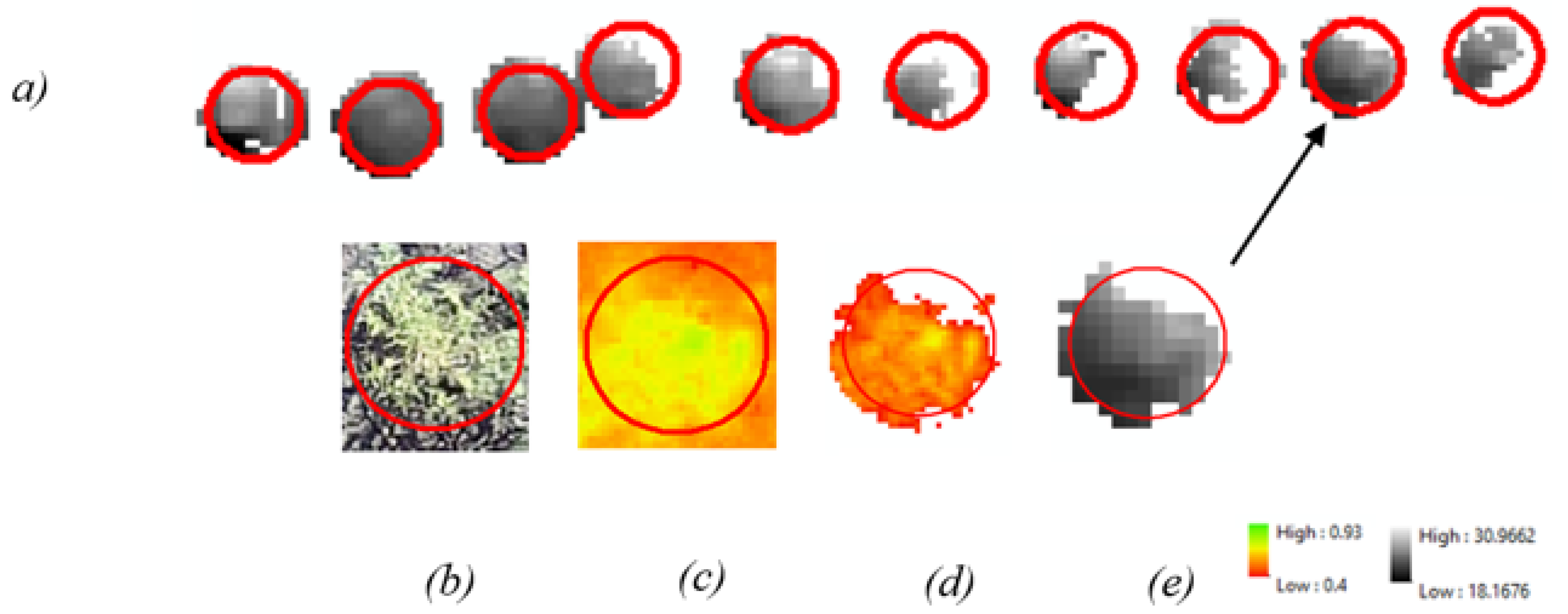
Once the images were gathered from the experiments, they were processed into mosaics before visualizing in ArcGIS Pro (ESRI, Redlands, CA, USA). The plant GPS data were then overlaid as point shapefiles. The Buffer tool in ArcGIS Pro was then used to create 12 cm buffer shapefiles around the centroid of the pots. The buffer size selection was empirical and it was decided by the specialists at NDSU. Buffers were inspected for accurate placement in the imagery and corrected if necessary. Buffers were then selected and separated into their own respective species using the Clip tool. The visual survival evaluation results were then added to the shapefile attribute table to further separate the buffers into resistant and susceptible biotypes within each species.
The buffers were then used to extract 12 cm diameter raster information from each image dataset, vastly reducing the amount of imagery so that only the plant locations would be subjected to further processes. This approach, however, still left a mixture of soil and vegetation within the buffers. To increase the extraction accuracy even further, the Extract by Attributes tool was used to extract pixels from the buffers that had an NDVI value greater than 0.4. This action removed the soil from the buffers so that only vegetation would be displayed. The NDVI output was then used to remove soil pixels from the thermal and multispectral raster using the Extract by Mask tool. The complete extraction process is illustrated in Figure 2.
Sets of buffers were created for each species and separated into six classes based on their resistance status. The classification was made as magnitude of glyphosate resistance where zero indicated dead plants while five indicated plants with no symptoms. The magnitude of resistance (MoR) indicated increasing resistance as the numbers go up from zero to five where one indicating more symptoms while four indicating lesser symptoms on plants.
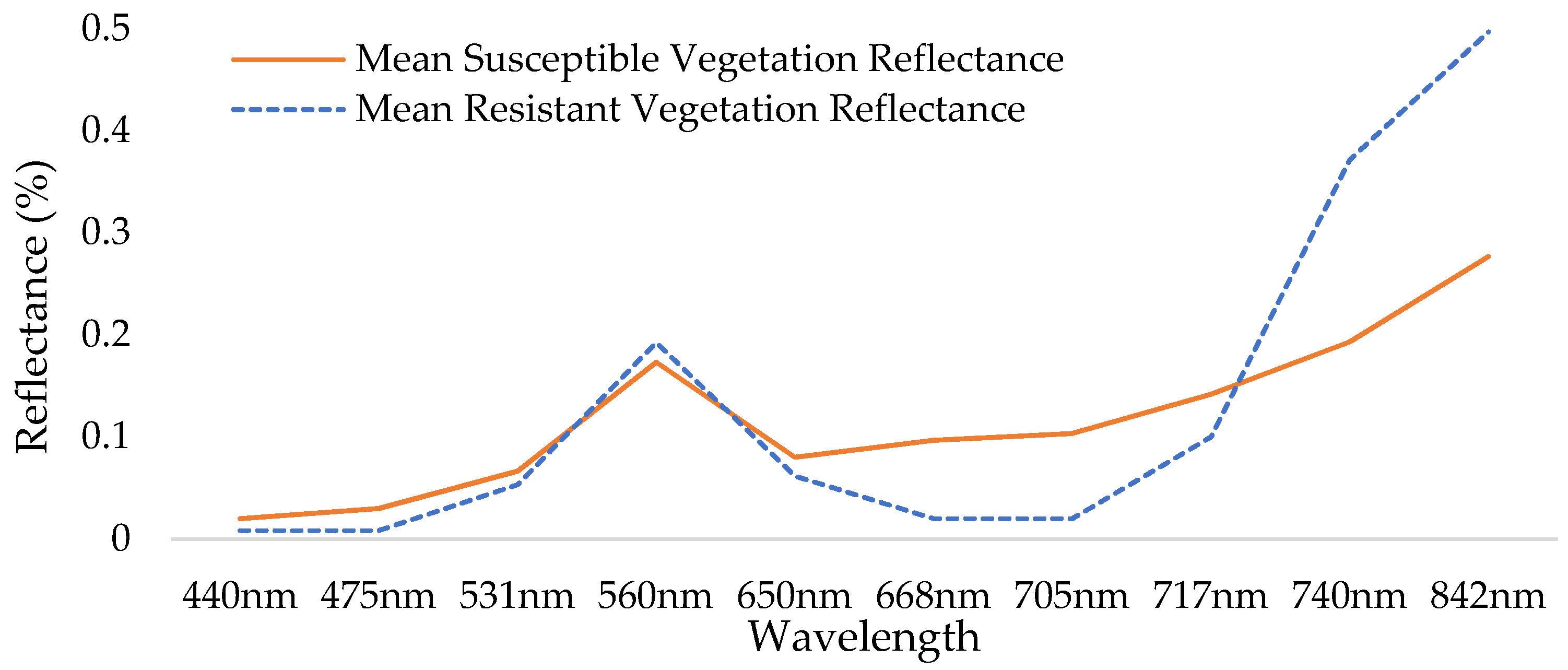
In addition to thermal extraction from the Zenmuse XT2, extractions of NDVI and a 3-band composite image from the Red-Edge MX Dual Camera system were also made to serve as comparisons. By using the Spectral Profile tool within ArcGIS, the reflectance of glyphosate-resistant vegetation and glyphosate-susceptible vegetation were compared at each of the ten bands provided by the Red-Edge MX Dual Camera system.

2.4. Raster Classification of Glyphosate-Resistant and Glyphosate Susceptible Weeds

Once the buffered and extracted datasets were created, they were then classified using the Image Classification Wizard in ArcGIS Pro. Training zones were created over the plant locations using the buffer shapefiles that were separated based upon resistance status and then conjoined to create a training template containing two classes: glyphosate-susceptible vegetation and the other being glyphosate-resistant vegetation. Each classification was performed on each species independent from one another except in the case of waterhemp and redroot pigweed. In addition to weed classifications, a classification was made between the Round-up Ready soybean and conventional Stutsman soybean at Casselton 8 DAA to see if thermal classification performance could be greatly improved when dealing with known opposing MoR ratings.
Pixel based image analysis was used to classify the biotypes. Three classification methods were used to classify each species raster dataset for each of the three days. Data were collected to compare classification accuracy between the imaging systems and classification methods. Maximum likelihood, random trees, and support vector machine were the three classification methods used [58,59,60]. The support vector machine classification method utilized only a subset of the pixels included in the raster datasets to act as training data for the classifier. The maximum samples per class was set to the default value of 500 pixels for each class. The random trees classifier similarly used only a subset of pixels but with a default value of 1000 pixels.

2.5. Accuracy Assessments of Thermal, NDVI, and Wavelength Composite Classifications

To test the accuracy of the generated classifications, the Create Accuracy Assessment tool within ArcGIS Pro was used to digitize ground truth points within each classification raster’s extents. Pixels that belonged to plants that were determined to be glyphosate-susceptible within the survival evaluation were assigned the value of 0, while pixels that belonged to a glyphosate-resistant plant were assigned a value of 1. Approximately 1000 points were used for every species. The points were then updated by recording the values of the point locations observed in the classification raster, which provided a shapefile with both ground truth and classification fields with raster values ranging from 0–1. The Compute Confusion Matrix tool was then used to observe the accuracy and kappa coefficient of each classification attempt. 
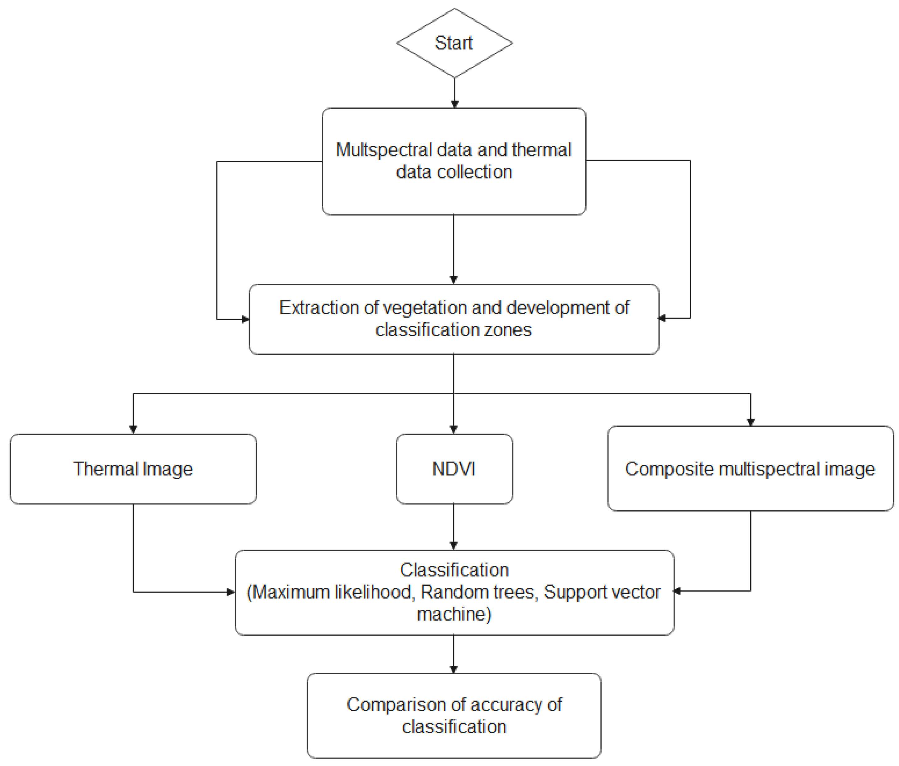
Figure 3 showed the image processing and prediction analysis steps for the weed classification in this study.

3. Results and Discussion

3.1. Post-Experiment Evaluation and Comparisons

Post-experiment visual evaluations that were performed 14 days after application (14 DAA) showed that varying degrees of glyphosate resistance occurred in the species. The MoR observed at the Casselton location are summarized where weeds are grouped based on their resistance status. Plants with MoR equal to or greater than 3 were considered resistant (Res) (Table 3).
The same source of seeds was used in both Casselton and Carrington locations. Therefore, the varying degrees of resistance observed at Casselton were also observed at Carrington, as expected. However, the efficacy of the herbicide was noticeably less at the Carrington site. This was because symptomology was seen as early as 2 DAA at the Casselton site but not seen until 6 DAA at the Carrington site. The rates of susceptibility observed at the Carrington location are summarized within Table 4.
The comparison between the reflectance of glyphosate-resistant vegetation and glyphosate-susceptible vegetation at each of the ten bands provided by the Red-Edge MX Dual Camera system can be seen in Figure 4. Wavelengths 842 nm, 705 nm, and 740 nm from the Red-Edge MX Dual Camera System were selected because large differences in reflectance were found at these wavelengths between glyphosate-resistant vegetation and glyphosate-susceptible vegetation. Wavelengths 842 nm, 740 nm, and 705 nm were subsequently used to create a composite image that served as a third image dataset for classification attempts.
A subset of the experiment datasets from the Casselton and Carrington locations at six days after glyphosate application are viewable in Figure 5 and Figure 6. Similar image datasets from every collection period and location were used throughout the experiment.

3.2. A Discussion on Raster Classification of Glyphosate Resistant and Glyphosate Susceptible Weeds

The MoR of resistance did not have any variation within the respective species as the waterhemp population was determined to be completely resistant to the glyphosate application while the redroot pigweed population was determined to be completely susceptible to the glyphosate application. That being said, waterhemp and redroot pigweed both are in the same genus of herbaceous plants (Amaranthus L.) commonly referred to as pigweeds [61]. Rather than sacrificing their presence in the study because of their unfavorable resistance statuses, the two species were paired together because of their close relation to each other. The waterhemp served as a glyphosate resistant population and redroot pigweed served as a susceptible population. This approach sacrificed the randomization schemes seen in kochia and ragweed, making thermal classification results unreliable due to spatial temperature differences of areas within the scene. NDVI and wavelength combination of 705 nm, 742 nm, and 842 nm was somewhat reliable as spectral reflectance of vegetation is more consistent despite its location within the scene as all plants received approximately the same amount of sunlight. Improvements in classification accuracy were observed across the total data collection period for each site with wavelength combination 705 nm, 740 nm, and 842 nm from the Red-Edge MX Dual Camera providing the highest accuracy and kappa coefficient results. This effect is expected, as the herbicide is provided more time to induce symptomology and gradually desiccate the susceptible population due to the inhibition of stomatal conductance often observed with glyphosate application [20].

3.3. Classification of Glyphosate-Resistant Kochia

The kappa coefficient values for kochia at 4 DAA suggested only slight agreement at best between the classification and ground truth fields of wavelength combination 705 nm, 740 nm, and 842 nm at the Casselton location (Table 5). The wavelengths in this classification fall within previously reported values in determining glyphosate-resistant kochia [62]. The random trees classifier performed the best at 4 DAA with an accuracy of 62.9%. At 6 DAA, performance slightly improved in all band options. Wavelength combination 705 nm, 740 nm, and 842 nm at the Casselton location with the random trees classifier once again achieved the highest classification accuracy and kappa coefficient results at this time period with values of 74% and 0.471, respectively. The 8 DAA kochia classification at Casselton once again improved in performance. The maximum likelihood classifier provided the highest performing result out of all classification attempts with an accuracy of 75.2% and a kappa coefficient of 0.487.
Thermal classifications for kochia were noticeably the lowest performing of the three tested band options. The highest performing thermal classification, which used the random trees method at 8 DAA was outperformed by all NDVI and wavelength combination 705 nm, 740 nm, and 842 nm classifications. This finding suggests that thermal canopy temperature was not a reliable predictor of glyphosate resistance in kochia and that multispectral data should be further investigated.

3.4. Classification of Glyphosate Resistant Ragweed

Generally, poor classification performance was seen in ragweed as well. Only 8 ragweed plants at the Carrington site succumbed to the glyphosate application and 22 survived. The weeds showed varying levels of resistance, which likely also reduced the classifier’s capability to distinguish between the two biotypes. Contrary to the Casselton site, a large number of susceptible ragweed dominated the Casselton site, leaving only 7 resistant weeds. The natural population of ragweed that was introduced to the study to increase population sizes was determined to be part of the cause for such varying numbers, but it can also be noted that the glyphosate symptomology appeared much sooner and more severely than at Carrington. Despite difficulties in the 4 DAA and 6 DAA data collections, a commendable classification was made via NDVI 8 DAA in Casselton, where the random trees classifier attained an accuracy of 87.2% with a kappa of 0.413 (Table 6). In order to determine the effectiveness of thermal data to identify glyphosate resistance in ragweed, it is necessary that more data be gathered.

3.5. Classification of Glyphosate Resistant Amaranth

The amaranth dataset (composed of resistant waterhemp and susceptible redroot pigweed) exhibited much higher accuracy and kappa scores for thermal classifications, although these values are likely inflated. The Carrington site’s thermal classifications likely received such high accuracy and kappa scores solely because of the two species’ spatial location within the scene. The resistant waterhemp population filled the interior of a soybean row with dense vegetation that was near canopy closure. The soybean canopy provided shelter for the waterhemp, while the redroot pigweed was positioned on the outside of a soybean row, where it was directly exposed to sunlight. The presence of shadows over vegetation provide a cooling effect to the waterhemp plant areas. Shaded areas received diffused solar radiation compared to areas in direct sunlight, leading to a significant temperature differential [25]. In addition to the difference in spatial location, the polarizing differences in MoR that were observed could also further cause an easily detectable temperature differential between the two species, where the resistant waterhemp canopies showed cooler temperatures than the susceptible redroot pigweed canopies.
It is possible that the difference in spatial location was not as much of a factor at the Casselton location as sunlight exposure was approximately the same for both species. Due to the north facing orientation of the plot, sunlight was provided parallel to the soybean rows at the time of data collection rather than across dense soybean rows as in Carrington. This reasoning could offer explanation as to why the Carrington location received higher accuracy results than Casselton. Regardless, this approach illustrates the powerful impact of spatial variability of temperature on classification accuracy using thermal sensors. Weeds that were placed only a few feet away from each other exhibited significantly different canopy temperatures because of different levels of exposure to sunlight. While the spatial variability and presence of crops could potentially impact the thermal readings, reflectance values from a multispectral sensor are less susceptible to the same degree of contamination as sunlight reflectance is the value being recorded and not temperature. Therefore, the superior performance shown by the multispectral sensors serves as another indicator that thermal classifications are not reliable. The results of the Amaranth classifications are summarized in Table 7.

3.6. Soybean Observation Results

An experiment for distinguishing glyphosate-resistant vegetation and glyphosate-susceptible vegetation was made using the conventional Stutsman soybean and Xtend2 Round-Up Ready soybean at the Casselton location. The observation made to investigate the classification accuracy attained when dealing with vegetation with known opposing MoR found that multispectral data generally show better potential for classification between glyphosate-resistant and glyphosate-susceptible vegetation. However, thermal classifications showed higher performance at 4 DAA than NDVI or the Band 579 (Table 8). This finding was unexpected, as thermal classifications for any of the weed species did not exhibit similar performance levels at this time interval. This outlier in classification performance could result from incorporating highly glyphosate-susceptible Stutsman soybean and glyphosate tolerant Xtend 2 Round Up Ready soybean. This degree of difference in resistance status is highly unlikely in natural populations of weeds as resistance to glyphosate is generally conferred at a low MoR (2 or 3) which is why high doses of herbicide are recommended to impede glyphosate resistance [26]. An additional suggestion for the increased performance is that the increased amount of vegetation area was able to be captured more effectively with the lower resolution thermal camera, thus encouraging segregation between classes [63]. The Zenmuse XT2 thermal camera provided 1.03 cm/pixel spatial resolution. The average leaf diameter of the soybean plants was 7 cm. The average leaf diameter that belonged to waterhemp and was only 2–3 cm. Therefore, it is possible that there were other reliable thermal signatures captured from soybean canopies than weed canopies [64]. Reliable soybean canopy temperature extraction has proven to be possible with spatial resolutions as high as 0.8 m when investigating stomatal closure due to drought conditions [18].
Overall, determining glyphosate-resistant weed species with UAV thermal sensing was not possible in field conditions. Our previous study on thermal sensing for glyphosate-resistant weed identification under greenhouse conditions also produced similar results and raised questions on how to improve its overall performance for future studies [22]. The experiment conditions and some of the parameters could be readjusted to further improve the performance such as consideration of different experiment size, UAV flight parameters, thermal sensors, and daylight conditions [65,66]. In addition, complementary measurements to thermal measurements could improve the overall efficiency of determining glyphosate-resistant weed species [49,50,51]. In this case, the multispectral measurements were more reliable than the thermal measurements on determining glyphosate resistance status, therefore a combined analysis of the two could provide more accurate results. Furthermore, shading issue in remote sensing is a well-known problem, especially for thermal sensing [67]. Improving abovementioned parameters could improve overall performance of UAV thermal sensing as well as help eliminate the concerns on temperature differences due to uneven solar radiance [68].
The multispectral sensing technology was specifically introduced in this research to explore the reliability of glyphosate-resistant weed identification in-field condition. Using various imaging technologies to identify weed in precision agriculture had been investigated by other researchers for at least a decade. In 2001, Rath and Hemming investigated computer vision-based weed identification under controlled lighting in-field conditions. The experiments showed that color features could help increase classification accuracy [69]. Later in 2016, Ortiz et al. used UAV imagery to extract patterns and features between and within crop row for weed mapping. The results showed that more than 91.5% of weed objects were classified in the sunflower field [70]. One of the most recent research that focused on weed mapping through UAV tested four independent classification algorithms for the creation of weed maps by combining automatic and manual methods for weed classification. The results showed that the automatic object-based classification method achieved the highest classification accuracy, resulting in an overall accuracy of 89.0% for subset “A” and 87.1% for subset “B”. With all the research mentioned above, they were more focused on the image detection methods, which is critical for weed identification [71]. However, in our research, we did not only focus on the method for image recognition and classification, but also on classification of glyphosate-resistant and glyphosate susceptible weed attributes. The latter focus served as the main objective for this research, which made significant contribution to weed control publications.

4. Conclusions

Cost-effective weed management strategy without promoting glyphosate-resistant weed biotypes requires distinguishing resistant and susceptible biotypes in the field conditions. Unmanned Aerial Vehicle (UAV)-assisted thermal and multispectral remote sensing could improve distinguishing glyphosate-susceptible and glyphosate-resistant weed populations based on canopy temperature and deep learning driven weed identification algorithms. However, the thermal imagery as a predictor for glyphosate resistance within weed populations did not perform well in this study. While technological advancements have provided increased resolutions in thermal systems, it was observed that higher resolution is needed to make thermal data more scalable. Normalized Difference Vegetation Index (NDVI) and a composite image comprised of 842 nm, 705 nm, and 740 nm wavelength imagery managed to provide better classification results than thermal data provided. However, classifications that performed within a single species to segregate glyphosate-resistant and glyphosate-susceptible biotypes of weeds still were not definitive. The high classification accuracy obtained in the cases of amaranth and soybean plants supports the notion that extreme differences in Mode of Resistance (MoR) are necessary for any reliable attempt to identify glyphosate-resistant vegetation regardless of using multispectral or thermal data as a predictor. Regardless of the limitations in the experiment design, the research could be a useful step towards identifying potential methods for further weed identification studies.

Author Contributions

Conceptualization, A.E. and X.S.; methodology, A.E.; software, A.E. and Y.Z.; validation, A.E., Y.Z. and C.K.; formal analysis, A.E.; investigation, A.E.; resources, X.S., Y.Z., M.O. and K.H.; data curation, A.E.; writing—original draft preparation, A.E.; writing—review and editing, C.K., Y.Z., M.O., K.H. and X.S.; visualization, A.E.; supervision, X.S.; project administration, X.S.; funding acquisition, X.S. All authors have read and agreed to the published version of the manuscript.

Funding

This material is based upon work partially supported by the U.S. Department of Agriculture, agreement number 58-6064-8-023. Any opinions, finding, conclusions or recommendations expressed in this publication are those of the author(s) and do not necessarily reflect the view of the U.S. Department of Agriculture. This research was also partially supported by the North Dakota State University Agricultural Experiment Station Precision Agriculture Fund FARG080010.

Institutional Review Board Statement

Not applicable.

Informed Consent Statement

Not applicable.

Data Availability Statement

The data presented in this study are available on request from the corresponding author. The data are not publicly available due to data format and size.

Conflicts of Interest

The authors declare no conflict of interest.

References

  1. Green, J.M. The benefits of herbicide-resistant crops. Pest Manag. Sci. 2012, 68, 1323–1331. [Google Scholar] [CrossRef] [PubMed]
  2. Oerke, E.C. Crop losses to pests. J. Agric. Sci. 2006, 144, 31–43. [Google Scholar] [CrossRef]
  3. Soltani, N.; Dille, J.A.; Burke, I.C.; Everman, W.J.; VanGessel, M.J.; Davis, V.M.; Sikkema, P.H. Potential Corn Yield Losses from Weeds in North America. Weed Technol. 2016, 30, 979–984. [Google Scholar] [CrossRef]
  4. Evans, J.A.; Tranel, P.J.; Hager, A.G.; Schutte, B.; Wu, C.; Chatham, L.A.; Davis, A.S. Managing the evolution of herbicide resistance. Pest Manag. Sci. 2016, 72, 74–80. [Google Scholar] [CrossRef] [PubMed]
  5. Christophers, M.J. Genetic Aspects of Herbicide-Resistant Weed Management. Weed Technol. 1999, 13, 647–652. [Google Scholar] [CrossRef]
  6. Pollegioni, L.; Schonbrunn, E.; Siehl, D. Molecular basis of glyphosate resistance—Different approaches through protein engineering. FEBS J. 2011, 278, 2753–2766. [Google Scholar] [CrossRef] [Green Version]
  7. Gage, K.L.; Krausz, R.F.; Walters, S.A. Emerging Challenges for Weed Management in Herbicide-Resistant Crops. Agriculture 2019, 9, 180. [Google Scholar] [CrossRef] [Green Version]
  8. Schütte, G.; Eckerstorfer, M.; Rastelli, V.; Reichenbecher, W.; Restrepo-Vassalli, S.; Ruohonen-Lehto, M.; Saucy, A.-G.W.; Mertens, M. Herbicide resistance and biodiversity: Agronomic and environmental aspects of genetically modified herbicide-resistant plants. Environ. Sci. Eur. 2017, 29, 5. [Google Scholar] [CrossRef] [Green Version]
  9. Hartzler, R. The Cost of Herbicide Resistance. Available online: https://crops.extension.iastate.edu/blog/bob-hartzler/cost-herbicide-resistance (accessed on 8 December 2019).
  10. Pause, M.; Raasch, F.; Marrs, C.; Csaplovics, E. Monitoring Glyphosate-Based Herbicide Treatment Using Sentinel-2 Time Series—A Proof-of-Principle. Remote Sens. 2019, 11, 2541. [Google Scholar] [CrossRef] [Green Version]
  11. Kanissery, R.; Gairhe, B.; Kadyampakeni, D.; Batuman, O.; Alferez, F. Glyphosate: Its Environmental Persistence and Impact on Crop Health and Nutrition. Plants 2019, 8, 499. [Google Scholar] [CrossRef] [Green Version]
  12. Gomes, M.P.; Le Manac’h, S.G.; Hénault-Ethier, L.; Labrecque, M.; Lucotte, M.; Juneau, P. Glyphosate-Dependent Inhibition of Photosynthesis in Willow. Front. Plant Sci. 2017, 8, 207. [Google Scholar] [CrossRef] [PubMed]
  13. Gaines, T.A.; Duke, S.O.; Morran, S.; Rigon, C.A.G.; Tranel, P.J.; Küpper, A.; Dayan, F.E. Mechanisms of evolved herbicide resistance. J. Biol. Chem. 2020, 295, 10307–10330. [Google Scholar] [CrossRef] [PubMed]
  14. Reddy, K.N.; Huang, Y.; Lee, M.A.; Nandula, V.K.; Fletcher, R.S.; Thomson, S.J.; Zhao, F. Glyphosate-resistant and glyphosate-susceptible Palmer amaranth (Amaranthus palmeri S. Wats.): Hyperspectral reflectance properties of plants and potential for classification. Pest Manag. Sci. 2014, 70, 1910–1917. [Google Scholar] [CrossRef] [PubMed]
  15. Shirzadifar, A.; Bajwa, S.; Nowatzki, J.; Bazrafkan, A. Field identification of weed species and glyphosate-resistant weeds using high resolution imagery in early growing season. Biosyst. Eng. 2020, 200, 200–214. [Google Scholar] [CrossRef]
  16. Xu, S.; Hossain, M.M.; Lau, B.B.Y.; To, T.Q.; Rawal, A.; Aldous, L. Total quantification and extraction of shikimic acid from star anise (llicium verum) using solid-state NMR and cellulose-dissolving aqueous hydroxide solutions. Sustain. Chem. Pharm. 2017, 5, 115–121. [Google Scholar] [CrossRef] [Green Version]
  17. Singh, V.; Rana, A.; Bishop, M.; Filippi, A.M.; Cope, D.; Rajan, N.; Bagavathiannan, M. Chapter Three—Unmanned aircraft systems for precision weed detection and management: Prospects and challenges. In Advances in Agronomy; Sparks, D.L., Ed.; Academic Press: Cambridge, MA, USA, 2020; Volume 159, pp. 93–134. [Google Scholar]
  18. Shirzadifar, A. Identification of Weed Species and Glyphosate-Resistant Weeds Using High Resolution UAS Images. Ph.D. Thesis, 2018. Available online: https://library.ndsu.edu/ir/handle/10365/29304 (accessed on 5 November 2021).
  19. Stoll, M.; Hamlyn, G.J. Thermal imaging as a viable tool for monitoring plant stress. OENO One 2007, 41, 77–84. [Google Scholar] [CrossRef]
  20. Picoli, G.; Carbonari, C.; Matos, A.; Rodrigues, L.; Velini, E. Influence of glyphosate on susceptible and resistant ryegrass populations to herbicide. Planta Daninha 2017, 35, e017163391. [Google Scholar] [CrossRef] [Green Version]
  21. Gonzalez-Dugo, V.; Lopez-Lopez, M.; Espadafor, M.; Orgaz, F.; Testi, L.; Zarco-Tejada, P.; Lorite, I.J.; Fereres, E. Transpiration from canopy temperature: Implications for the assessment of crop yield in almond orchards. Eur. J. Agron. 2019, 105, 78–85. [Google Scholar] [CrossRef]
  22. Eide, A.; Zhang, Y.; Koparan, C.; Stenger, J.; Ostlie, M.; Howatt, K.; Bajwa, S.; Sun, X. Image based thermal sensing for glyphosate resistant weed identification in greenhouse conditions. Comput. Electron. Agric. 2021, 188, 106348. [Google Scholar] [CrossRef]
  23. Johnson, W.G.; Owen, M.D.K.; Kruger, G.R.; Young, B.G.; Shaw, D.R.; Wilson, R.G.; Wilcut, J.W.; Jordan, D.L.; Weller, S.C. U.S. Farmer Awareness of Glyphosate-Resistant Weeds and Resistance Management Strategies. Weed Technol. 2009, 23, 308–312. [Google Scholar] [CrossRef]
  24. Foresman, C.; Glasgow, L. US grower perceptions and experiences with glyphosate-resistant weeds. Pest Manag. Sci. 2008, 64, 388–391. [Google Scholar] [CrossRef]
  25. Beckie, H.J.; Sikkema, P.H.; Soltani, N.; Blackshaw, R.E.; Johnson, E.N. Environmental Impact of Glyphosate-Resistant Weeds in Canada. Weed Sci. 2014, 62, 385–392. [Google Scholar] [CrossRef]
  26. Deng, L.; Mao, Z.; Li, X.; Hu, Z.; Duan, F.; Yan, Y. UAV-based multispectral remote sensing for precision agriculture: A comparison between different cameras. ISPRS J. Photogramm. Remote Sens. 2018, 146, 124–136. [Google Scholar] [CrossRef]
  27. Roslim, M.H.M.; Juraimi, A.S.; Che’Ya, N.N.; Sulaiman, N.; Manaf, M.N.H.A.; Ramli, Z.; Motmainna, M. Using remote sensing and an unmanned aerial system for weed management in agricultural crops: A review. Agronomy 2021, 11, 1809. [Google Scholar] [CrossRef]
  28. Qi, H.; Wu, Z.; Zhang, L.; Li, J.; Zhou, J.; Jun, Z.; Zhu, B. Monitoring of peanut leaves chlorophyll content based on drone-based multispectral image feature extraction. Comput. Electron. Agric. 2021, 187, 106292. [Google Scholar] [CrossRef]
  29. The Science Behind MicaSense—MicaSense. 2017. Available online: https://micasense.com/the-science-behind-micasense/ (accessed on 5 November 2021).
  30. Liu, J.; Chen, P.; Xu, X. Estimating wheat coverage using multispectral images collected by unmanned aerial vehicles and a new sensor. In Proceedings of the 2018 7th International Conference on Agro-Geoinformatics (Agro-Geoinformatics), Hangzhou, China, 6–9 August 2018; pp. 1–5. [Google Scholar]
  31. Dual Camera Imaging System—MicaSense. Available online: https://micasense.com/dual-camera-system/ (accessed on 5 November 2021).
  32. Chawade, A.; Ham, J.v.; Blomquist, H.; Bagge, O.; Alexandersson, E.; Ortiz, R. High-Throughput Field-Phenotyping Tools for Plant Breeding and Precision Agriculture. Agronomy 2019, 9, 258. [Google Scholar] [CrossRef] [Green Version]
  33. Sankaran, S.; Khot, L.R.; Espinoza, C.Z.; Jarolmasjed, S.; Sathuvalli, V.R.; Vandemark, G.J.; Miklas, P.N.; Carter, A.H.; Pumphrey, M.O.; Knowles, N.R.; et al. Low-altitude, high-resolution aerial imaging systems for row and field crop phenotyping: A review. Eur. J. Agron. 2015, 70, 112–123. [Google Scholar] [CrossRef]
  34. Xu, R.; Li, C.; Paterson, A.H. Multispectral imaging and unmanned aerial systems for cotton plant phenotyping. PLoS ONE 2019, 14, e0205083. [Google Scholar] [CrossRef] [PubMed] [Green Version]
  35. Fernández, C.I.; Leblon, B.; Haddadi, A.; Wang, K.; Wang, J. Potato Late Blight Detection at the Leaf and Canopy Levels Based in the Red and Red-Edge Spectral Regions. Remote Sens. 2020, 12, 1292. [Google Scholar] [CrossRef] [Green Version]
  36. Thompson, L.J.; Puntel, L.A. Transforming Unmanned Aerial Vehicle (UAV) and Multispectral Sensor into a Practical Decision Support System for Precision Nitrogen Management in Corn. Remote Sens. 2020, 12, 1597. [Google Scholar] [CrossRef]
  37. Dyrmann, M.; Mortensen, A.; Midtiby, H.; Jørgensen, R. Pixel-Wise Classification of Weeds and Crops in Images by Using a Fully Convolutional Neural Network. 2016. Available online: https://www.semanticscholar.org/paper/Pixel-wise-classification-of-weeds-and-crops-in-by-Dyrmann-Mortensen/393d4bbb92e5ce5e308ad61a771cc2015b342d5d (accessed on 5 November 2021).
  38. Crusiol, L.G.T.; Nanni, M.R.; Furlanetto, R.H.; Sibaldelli, R.N.R.; Cezar, E.; Mertz-Henning, L.M.; Nepomuceno, A.L.; Neumaier, N.; Farias, J.R.B. UAV-based thermal imaging in the assessment of water status of soybean plants. Int. J. Remote Sens. 2019, 41, 3243–3265. [Google Scholar] [CrossRef]
  39. Zhang, W.; Yi, S.-h.; Qin, Y.; Shangguan, D.-h.; Qin, Y. Analysis of features and influencing factors of alpine meadow surface temperature based on UAV thermal thermography. Acta Prataculturae Sin. 2021, 30, 15. [Google Scholar]
  40. Pineda, M.; Barón, M.; Pérez-Bueno, M.-L. Thermal imaging for plant stress detection and phenotyping. Remote Sens. 2021, 13, 68. [Google Scholar] [CrossRef]
  41. Awais, M.; Li, W.; Cheema, M.J.M.; Hussain, S.; AlGarni, T.S.; Liu, C.; Ali, A. Remotely sensed identification of canopy characteristics using UAV-based imagery under unstable environmental conditions. Environ. Technol. Innov. 2021, 22, 101465. [Google Scholar] [CrossRef]
  42. Sagan, V.; Maimaitijiang, M.; Sidike, P.; Eblimit, K.; Peterson, K.T.; Hartling, S.; Esposito, F.; Khanal, K.; Newcomb, M.; Pauli, D.; et al. UAV-Based High Resolution Thermal Imaging for Vegetation Monitoring, and Plant Phenotyping Using ICI 8640 P, FLIR Vue Pro R 640, and thermoMap Cameras. Remote Sens. 2019, 11, 330. [Google Scholar] [CrossRef] [Green Version]
  43. Botyanszka, L. A Review of Imaging and Sensing Technologies for Field Phenotyping. Acta Hortic. Regiotect. 2021, 24, 58–69. [Google Scholar] [CrossRef]
  44. Gelasakis, A.I.; Kalogianni, A.I.; Moschovas, M.; Tsimpouri, E.; Pnevmatikos, T.; Bossis, I.; Arsenos, G.; Simitzis, P. Evaluation of Infrared Thermography for the Detection of Footrot and White Line Disease Lesions in Dairy Sheep. Vet. Sci. 2021, 8, 219. [Google Scholar] [CrossRef]
  45. Zhang, C.; Valente, J.; Kooistra, L.; Guo, L.; Wang, W. Orchard management with small unmanned aerial vehicles: A survey of sensing and analysis approaches. Precis. Agric. 2021, 22, 2007–2052. [Google Scholar] [CrossRef]
  46. Ballester, C.; Zarco-Tejada, P.J.; Nicolás, E.; Alarcón, J.J.; Fereres, E.; Intrigliolo, D.S.; Gonzalez-Dugo, V. Evaluating the performance of xanthophyll, chlorophyll and structure-sensitive spectral indices to detect water stress in five fruit tree species. Precis. Agric. 2018, 19, 178–193. [Google Scholar] [CrossRef]
  47. Gonzalez-Dugo, V.; Zarco-Tejada, P.; Nicolás, E.; Nortes, P.A.; Alarcón, J.J.; Intrigliolo, D.S.; Fereres, E. Using high resolution UAV thermal imagery to assess the variability in the water status of five fruit tree species within a commercial orchard. Precis. Agric. 2013, 14, 660–678. [Google Scholar] [CrossRef]
  48. Gómez-Candón, D.; Virlet, N.; Labbé, S.; Jolivot, A.; Regnard, J.-L. Field phenotyping of water stress at tree scale by UAV-sensed imagery: New insights for thermal acquisition and calibration. Precis. Agric. 2016, 17, 786–800. [Google Scholar] [CrossRef]
  49. Zhu, W.; Sun, Z.; Huang, Y.; Yang, T.; Li, J.; Zhu, K.; Zhang, J.; Yang, B.; Shao, C.; Peng, J.; et al. Optimization of multi-source UAV RS agro-monitoring schemes designed for field-scale crop phenotyping. Precis. Agric. 2021, 22, 1768–1802. [Google Scholar] [CrossRef]
  50. Calderón, R.; Montes-Borrego, M.; Landa, B.B.; Navas-Cortés, J.A.; Zarco-Tejada, P.J. Detection of downy mildew of opium poppy using high-resolution multi-spectral and thermal imagery acquired with an unmanned aerial vehicle. Precis. Agric. 2014, 15, 639–661. [Google Scholar] [CrossRef]
  51. Bellvert, J.; Zarco-Tejada, P.J.; Girona, J.; Fereres, E. Mapping crop water stress index in a ‘Pinot-noir’ vineyard: Comparing ground measurements with thermal remote sensing imagery from an unmanned aerial vehicle. Precis. Agric. 2014, 15, 361–376. [Google Scholar] [CrossRef]
  52. Martínez, J.; Egea, G.; Agüera, J.; Pérez-Ruiz, M. A cost-effective canopy temperature measurement system for precision agriculture: A case study on sugar beet. Precis. Agric. 2017, 18, 95–110. [Google Scholar] [CrossRef]
  53. Ohana-Levi, N.; Ben-Gal, A.; Peeters, A.; Termin, D.; Linker, R.; Baram, S.; Raveh, E.; Paz-Kagan, T. A comparison between spatial clustering models for determining N-fertilization management zones in orchards. Precis. Agric. 2021, 22, 99–123. [Google Scholar] [CrossRef]
  54. Zhao, B.; Adama, T.; Ata-Ul-Karim, S.T.; Guo, Y.; Liu, Z.; Xiao, J.; Liu, Z.; Qin, A.; Ning, D.; Duan, A. Recalibrating plant water status of winter wheat based on nitrogen nutrition index using thermal images. Precis. Agric. 2021. [Google Scholar] [CrossRef]
  55. Delavarpour, N.; Koparan, C.; Nowatzki, J.; Bajwa, S.; Sun, X. A Technical Study on UAV Characteristics for Precision Agriculture Applications and Associated Practical Challenges. Remote Sens. 2021, 13, 1204. [Google Scholar] [CrossRef]
  56. Prochnow, N.D.; Lunde, N.J.; Terry, W.J.; Opdahl, D.P. Soil Survey of Cass County Area, North Dakota; Soil Conversation Service, United States Department of Agriculture: Washington, DC, USA, 1985.
  57. Morrison, M. Soil Survey of Foster County, North Dakota; Soil Conversation Service, United States Department of Agriculture: Washington, DC, USA, 1995.
  58. Cortes, C.; Vapnik, V. Support-vector networks. Mach. Learn. 1995, 20, 273–297. [Google Scholar] [CrossRef]
  59. Enders, C.K. Maximum Likelihood Estimation. In Encyclopedia of Statistics in Behavioral Science; 2005; Available online: https://onlinelibrary.wiley.com/doi/10.1002/0470013192.bsa174 (accessed on 5 November 2021).
  60. Breiman, L. Random Forests. Mach. Learn. 2001, 45, 5–32. [Google Scholar] [CrossRef] [Green Version]
  61. Ikley, J.; Jenks, B. Identification, Biology and Control of Palmer Amaranth and Waterhemp in North Dakota; Research Extention; North Dakota State University: Fargo, ND, USA, 2019. [Google Scholar]
  62. Paul, W.N.; Joseph, A.S.; Prashant, J.; Bryan, S.; Andrew, D.; Vipan, K. Discrimination of herbicide-resistant kochia with hyperspectral imaging. J. Appl. Remote Sens. 2018, 12, 1–10. [Google Scholar] [CrossRef] [Green Version]
  63. Way, R.G.; Lapalme, C.M. Does tall vegetation warm or cool the ground surface? Constraining the ground thermal impacts of upright vegetation in northern environments. Environ. Res. Lett. 2021, 16, 054077. [Google Scholar] [CrossRef]
  64. Leigh, A.; Sevanto, S.; Close, J.D.; Nicotra, A.B. The influence of leaf size and shape on leaf thermal dynamics: Does theory hold up under natural conditions? Plant Cell Environ. 2017, 40, 237–248. [Google Scholar] [CrossRef] [PubMed]
  65. Sobrino, J.A.; Julien, Y. Time Series Corrections and Analyses in Thermal Remote Sensing. In Thermal Infrared Remote Sensing: Sensors, Methods, Applications; Kuenzer, C., Dech, S., Eds.; Springer: Dordrecht, The Netherlands, 2013; pp. 267–285. [Google Scholar]
  66. Jin, M.; Liang, S. An Improved Land Surface Emissivity Parameter for Land Surface Models Using Global Remote Sensing Observations. J. Clim. 2006, 19, 2867–2881. [Google Scholar] [CrossRef]
  67. Gillies, R.R.; Carlson, T.N. Thermal Remote Sensing of Surface Soil Water Content with Partial Vegetation Cover for Incorporation into Climate Models. J. Appl. Meteorol. Climatol. 1995, 34, 745–756. [Google Scholar] [CrossRef] [Green Version]
  68. Kawamura, K.; Watanabe, N.; Sakanoue, S.; Inoue, Y. Estimating forage biomass and quality in a mixed sown pasture based on partial least squares regression with waveband selection. Grassl. Sci. 2008, 54, 131–145. [Google Scholar] [CrossRef]
  69. Hemming, J.; Rath, T. PA—Precision agriculture: Computer-vision-based weed identification under field conditions using controlled lighting. J. Agric. Eng. Res. 2001, 78, 233–243. [Google Scholar] [CrossRef] [Green Version]
  70. Pérez-Ortiz, M.; Peña, J.M.; Gutiérrez, P.A.; Torres-Sánchez, J.; Hervás-Martínez, C.; López-Granados, F. Selecting patterns and features for between-and within-crop-row weed mapping using UAV-imagery. Expert Syst. Appl. 2016, 47, 85–94. [Google Scholar] [CrossRef] [Green Version]
  71. Gašparović, M.; Zrinjski, M.; Barković, Đ.; Radočaj, D. An automatic method for weed mapping in oat fields based on UAV imagery. Comput. Electron. Agric. 2020, 173, 105385. [Google Scholar] [CrossRef]
Figure 1. NDSU experiment sites represented in maps including weed species (top); (1) Casselton experiment site (bottom left) and (2) Carrington Experiment site (bottom right).
Remotesensing 13 04606 g001
Figure 2. The complete extraction process: (a) Extracted thermal data from kochia at the Casselton location. (b) RGB image of kochia for reference. (c) NDVI of kochia prior to 0.4-pixel value extraction. (d) NDVI mask containing pixels that score over 0.4 (e) NDVI mask applied to thermal data.
Remotesensing 13 04606 g002
Figure 3. Image processing and predicition analysis steps for weed classification.
Remotesensing 13 04606 g003
Figure 4. Spectral profile illustrating differences seen at 705 nm, 740 nm, and 842 nm between glyphosate-resistant vegetation and glyphosate-susceptible vegetation within the scene.
Remotesensing 13 04606 g004
Figure 5. Image datasets from Casselton at 6 days after glyphosate application (6 DAA) used in classification models. (a) Shapefiles denoting species and biotype location within the scene. (b) Thermal image dataset. (c) NDVI image dataset. (d) Composite Image Dataset for all wavelengths of the multispectral image (RRPW: Redroot Pigweed).
Remotesensing 13 04606 g005
Figure 6. Image datasets from Carrington at 6 days after glyphosate application (6 DAA) used in classification models. (a) Shapefiles denoting species and biotype location within the scene. (b) Thermal image dataset. (c) NDVI image dataset. (d) Composite Image Dataset for all wavelengths of the multispectral image (RRPW: Redroot Pigweed).
Remotesensing 13 04606 g006
Table 1. Weather conditions during data collection.
SiteDays after ApplicationCollection TimeAir Temp (°C)Relative Humidity (%)Solar Radiation (Lys)
Casselton410:30–11:3021.777414.5
610:30–11:3023.315561
810:30–11:3022.6877.537.5
Carrington410:30–11:3023.736552
610:30–11:3022.398033
Table 2. Unmanned Aerial Vehicle (UAV) flight operation summary.
Equipment and ParametersCamera Type
MultispectralThermal
UAV ModelDJI M600DJI M600
SensorMicasense Red-Edge Dual CameraZenmuse XT2 Thermal Camera
Pixel Resolution1280 × 960 640 × 512
Focal Length5.4 mm25 mm
Channels444, 475, 531, 560, 650, 668, 705, 717,740, 842 (nm)7.5–13.5 (μm)
Average altitude10 m8 m
Ground Spatial Distance0.71 cm1.03 cm
Forward overlap75%+80%
Side overlap75%+80%
FOV47.2° HFOV25° HFOV
Table 3. Casselton Plant Survival Evaluation at 14 DAA.
Species RatingMagnitude of Resistance# Observed
012345Susc.Res.
Kochia2112210663522
Ragweed42100025527
Waterhemp00001545060
Redroot Pigweed5280000600
Magnitude of Resistance: 0 = Dead Plants 5 = Alive Plants with no Symptoms.
Table 4. Carrington Plant Survival Evaluation at 14 DAA.
Species RatingMagnitude of Resistance# Observed
012345Susc.Res.
Kochia171779192535
Ragweed2337105822
Waterhemp00001842060
Redroot Pigweed40200000600
Magnitude of Resistance: 0 = Dead Plants 5 = Alive Plants with no Symptoms.
Table 5. Kochia Classification Performance Summary.
CarringtonCasselton
4 DAA 16 DAA 4 DAA 6 DAA 8 DAA
Band SelectionMethodAccuracyKappaAccuracyKappaAccuracyKappaAccuracyKappaAccuracyKappa
ThermalML 20.5910.0890.5760.1510.5760.1330.5770.1610.5790.17
RT 30.5070.0150.5890.1620.5480.0870.580.1630.6220.22
SVM 40.5420.1020.5870.1770.497−0.0040.5630.1260.6020.181
NDVI 5ML0.5720.040.6370.2860.5590.0110.6380.2760.6540.283
RT0.5720.040.6060.1150.6050.1790.6670.3170.7240.401
SVM0.5660.070.6230.2570.5880.1770.6660.3140.7260.388
Band Combo 705 nm, 740 nm, & 842 nmML0.5840.1670.6730.30.6090.2240.6910.3850.7520.487
RT0.5910.1340.7270.4530.6290.2580.740.4710.7420.463
SVM0.5840.1480.6670.3340.5770.190.7060.3720.7480.482
1 DAA: Days After Application, 2 ML: Maximum Likelihood, 3 RT: Random Trees, 4 SVM: Support Vector Machine, 5 NDVI: Normalized Difference Vegetation Index.
Table 6. Ragweed Classification Performance Summary.
CarringtonCasselton
4 DAA 1 6 DAA 4 DAA 6 DAA 8 DAA
Band SelectionMethodAccuracyKappaAccuracyKappaAccuracyKappaAccuracyKappaAccuracyKappa
ThermalML 20.5910.0890.4770.0450.582−0.0570.622−0.0460.430.071
RT 30.5070.0150.6430.250.5680.130.5140.0510.6270.119
SVM 40.5420.1020.4840.060.5920.0520.4420.020.5620.055
NDVI 5ML0.320.030.3290.0310.704−0.0870.6420.0990.7280.179
RT0.4830.0560.5740.1270.5620.050.6430.1740.7780.27
SVM0.4410.0220.5650.1190.540.0660.6890.1240.8720.413
Band Combo 705 nm, 740 nm, & 842 nmML0.4280.0670.290.0360.5520.0960.7110.1570.7610.246
RT0.6180.250.6560.30.6350.1130.7670.370.7690.303
SVM0.5640.1910.6330.2630.5360.0710.7550.2310.7670.278
1 DAA: Days After Application, 2 ML: Maximum Likelihood, 3 RT: Random Trees, 4 SVM: Support Vector Machine, 5 NDVI: Normalized Difference Vegetation Index.
Table 7. Amaranth Classification Performance Summary.
CarringtonCasselton
4 DAA 1 6 DAA 4 DAA 6 DAA 8 DAA
Band SelectionMethodAccuracyKappaAccuracyKappaAccuracyKappaAccuracyKappaAccuracyKappa
ThermalML 20.7780.5540.7070.4060.7750.4570.7830.4890.70.274
RT 30.7930.5870.9560.9120.7210.3890.7450.430.6780.177
SVM 40.7960.5920.920.840.790.4740.7960.4990.6510.278
NDVI 5ML0.7690.5350.8650.7290.9710.9350.9690.9390.9230.8
RT0.7270.4540.8690.7370.9670.9260.9760.9440.9350.81
SVM0.7790.5580.8610.7220.9720.9360.980.9540.9190.796
Band Combo 705 nm, 740 nm, & 842 nmML0.7780.5540.9110.8220.9770.9470.9420.8560.9350.82
RT0.7960.5920.8360.6710.9670.9260.9880.9720.9270.81
SVM0.7930.5870.9070.8130.970.9320.9860.9680.9190.796
1 DAA: Days After Application, 2 ML: Maximum Likelihood, 3 RT: Random Trees, 4 SVM: Support Vector Machine, 5 NDVI: Normalized Difference Vegetation Index.
Table 8. Casselton Soybean Classification Performance Summary.
4 DAA 1 6 DAA 8 DAA
Band SelectionMethodAccuracyKappaAccuracyKappaAccuracyKappa
ThermalML 20.9420.880.820.620.8860.76
RT 30.9180.830.770.520.9080.81
SVM 40.9360.870.790.560.8890.77
NDVI 5ML0.7940.550.9440.890.9770.95
RT0.710.410.9350.860.9810.96
SVM0.7420.450.9410.880.9830.96
Band Combo 705 nm, 740 nm, & 842 nmML0.8240.6360.9530.90.9870.972
RT0.820.640.9070.8080.9780.954
SVM0.8240.650.9630.9220.9810.959
1 DAA: Days After Application, 2 ML: Maximum Likelihood, 3 RT: Random Trees, 4 SVM: Support Vector Machine, 5 NDVI: Normalized Difference Vegetation Index.
Publisher’s Note: MDPI stays neutral with regard to jurisdictional claims in published maps and institutional affiliations.

