Abstract
Advanced machine learning techniques have been used in remote sensing (RS) applications such as crop mapping and yield prediction, but remain under-utilized for tracking crop progress. In this study, we demonstrate the use of agronomic knowledge of crop growth drivers in a Long Short-Term Memory-based, domain-guided neural network (DgNN) for in-season crop progress estimation. The DgNN uses a branched structure and attention to separate independent crop growth drivers and captures their varying importance throughout the growing season. The DgNN is implemented for corn, using RS data in Iowa, U.S., for the period 2003–2019, with United States Department of Agriculture (USDA) crop progress reports used as ground truth. State-wide DgNN performance shows significant improvement over sequential and dense-only NN structures, and a widely-used Hidden Markov Model method. The DgNN had a 4.0% higher Nash-Sutcliffe efficiency over all growth stages and 39% more weeks with highest cosine similarity than the next best NN during test years. The DgNN and Sequential NN were more robust during periods of abnormal crop progress, though estimating the Silking–Grainfill transition was difficult for all methods. Finally, Uniform Manifold Approximation and Projection visualizations of layer activations showed how LSTM-based NNs separate crop growth time-series differently from a dense-only structure. Results from this study exhibit both the viability of NNs in crop growth stage estimation (CGSE) and the benefits of using domain knowledge. The DgNN methodology presented here can be extended to provide near-real time CGSE of other crops.
1. Introduction
The increase in synchrony of global crop production and frequency of climate change-driven abnormal weather events is leading to higher variance in crop yields [1,2,3]. Most staple food crops are more vulnerable to yield loss in specific stages of growth, and as such, accurate crop growth stage estimation (CGSE) is vital to track crop growth at different spatial scales—local, regional, and national—and anticipate and mitigate the effects of variable harvest. High-resolution Remote Sensing (RS) data have been successfully employed to track crop growth at regional scales; however, current methods for CGSE utilize curve-fitting and simplistic Machine Learning (ML) models cannot describe the more complex relationships between crop growth drivers and crop growth stage progress [4,5,6,7,8]. Many of these methods require full-season data and do not provide in-season CGSE information.
Advanced ML models have found success in applications such as crop-cover mapping/classification and yield estimation [9,10,11,12,13], but these models have yet to been applied for in-season CGSE. Whereas methods such as Neural Networks (NNs) have been used in crop mapping, for which researchers can utilize crop cover maps [14] to retrieve millions of crop cover examples per year, field-level crop growth stage (CGS) data is not publicly available and producing field scale ground truth data via field studies is prohibitively expensive. As such, large scale CGSE research relies on local and regional level crop progress data for ground truth. Even for the longest continually running sub-weekly temporal resolution remote sensing (RS) sensors (e.g., MODIS), there are only 21 full growing seasons of crop growth data. Constructing accurate, in-season ML approaches from such limited data is difficult, particularly with few example seasons of abnormal weather. In addition, many crop growth studies estimate events such as ‘start of season’, ‘peak of season’, ‘end of season’, etc. [6,7], even though these events do not really describe phenological progress, and knowledge of their timing may not be actionable.
Recently, domain knowledge has been used to improve the performance of ML techniques in applied research using techniques collectively known as Theory-guide Machine Learning (TgML) [15,16]. TgML techniques include the use of physical models outputs [17], the integration of known domain limits into ML loss functions [18], and the designing of NN structures that reflect how variables interact within a real physical system [19]. For example, recent studies in agriculture such as [20] have integrated crop simulation models into ML methods for yield prediction; however, crop simulation model-based in-season CGSE is impractical, as calibrated simulation parameters for the latest cultivars and in situ planting/harvest dates are not readily available, and ML methods have been shown to outperform un-calibrated crop simulation models in rice CGSE [21].
TgML techniques have been shown to reduce the amount of data required to reach a given level of performance [15], and Theory-guided Neural Networks have begun to significantly improve upon current state-of-the-art methods in applications such as [22,23]. NNs have shown great promise in agricultural RS studies (e.g., [11,12]), but TgML methods have yet to fully utilize significant disciplinary advances in agriculture over the last two to three decades. The goal of this study is to understand the impact of incorporating domain knowledge into NN design for in-season CGSE at regional scales. Specifically, the objective of the study is to develop a Domain-guided NN (DgNN) that separates independent growth drivers and compare its performance to sequential NN structures of equivalent complexity. The TgML approach in this study is demonstrated for regional CGSE in field corn, which is one of the most cultivated crops in the world [24]. The methodology here, when paired with adequate crop mapping techniques, can be extended to track in-season growth of other crops.
2. Materials and Methods
2.1. Study Area and Data
This study was conducted in the state of Iowa, US, from 2003 to 2019. The state consists of nine separate Agricultural Statistical Districts (ASDs) (see Figure 1) and had an average of 13.4 million acres of corn under cultivation across the study period [25].
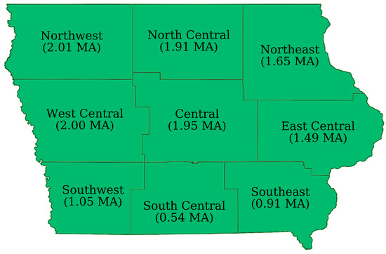
Figure 1.
Agricultural Statistical Districts in Iowa with average corn acreage planted over the study period in million acres (MA) [25].
Location of corn fields within the study region were obtained from the Corn-Soy Data Layer (CSDL) [26] for 2003–2007 and from the USDA Crop Data Layer (CDL) from 2008–2019 [14]. In Iowa, corn is typically planted in mid April/early May (week of year (WOY) 15–24), reaches its reproductive stages around late June (WOY 27 onward), and is harvested from early September through late November (WOY 36–48). Weekly USDA-NASS Crop Progress Reports (CPRs), generated from grower and crop assessor surveys, were used as ground truth. CPR progress stages include Planted, Emerged, Silking, Dough, Dent, Mature, and Harvested. In this study, the Planted stage was replaced with Pre-Emergence, a placeholder progress stage that represents all crop/field states prior to emergence, and the Dough and Dent stages were combined as Grainfill. CGSE requires both canopy growth information and meteorological data. This study used ASD-wide means and standard deviations of field-level RS and other data shown in Table 1. Fields in each ASD were selected from the CSDL and CDL based on size and boundary criteria (see Figure 2).

Table 1.
Remote sensing, meteorological, and soil inputs used in this study.
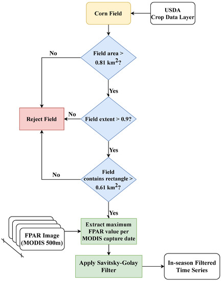
Figure 2.
Field selection and processing of MODIS FPAR images.
Micro-meteorological observations obtained from DayMet were used to compute field-level accumulated growing degree days (AGDD), which is a measure of accumulated temperature required for crop growth. AGDD is used to model progression through different corn growth stages, both in remote sensing studies and in mechanistic models [4,8,27]. The total number of growing degree days (GDD) for a single 24 h period is calculated using the function:
where is lower value of daily maximum temperature and 34 °C, is the minimum recorded daily temperature, and is the minimum temperature above which GDD is accumulated, set to 8 °C [28]. AGDD is a running total of daily GDD values, and in this study it is calculated from April 8th of a given year, which is the date prior to first planting during the study period. Solar radiation inputs were converted from W/m2 to MJ/m2/week using day length taken from DayMet to incorporate photoperiod information. Saturated hydraulic conductivities and bulk densities at field centroids from the CSDL and CDL were combined to obtain ASD-wide means and standard deviations.
To measure canopy growth, 4-day MODIS Fraction of absorbed Photosynthetically Activate Radiation (FPAR) values for each field within an ASD were filtered to produce daily time series data following the Savitsky-Golay (SG) filter method for NDVI used in [32]. In this study, the SG filter parameters were m = 40, d = 1 for long-term change trend fitting and m = 4, d = 1 for the main FPAR time series, where 2m + 1 is the moving filter size and d is the degree of the smoothing polynomial. To simulate in-season availability of FPAR data, the values were filtered independently up to each in-season cut-off week. FPAR values for a given week vary slightly as the season progresses and more data is included within the long-term filtering window. Noise filter adaptions to the existing SG method included rejecting points prior to September with an absolute gradient of >0.3 from the previous value, the earliest harvest over the study period. These adaptions prevented noisy, phenologically unrealistic data from being included in the moving filter window. It should be noted that while this filtering system is effective for a uni-modal crop such as corn, it may not be effective for crops with more complex seasonal FPAR patterns such as winter wheat, where higher polynomial filter parameters may be required.
2.2. Data Standardization
Since CPRs are released every Monday from data collected during the prior week, weekly meteorological data were obtained by aggregating field-scale daily data from Monday–Sunday. The dataset spanned 38 weeks, WOY 13–51, encompassing the earliest planting and latest harvest reported during the study period. To simulate in-season monitoring, one time series was produced from pre-emergence to the ‘current’ week per field, totaling 39 time series. Field-level time series for each input were then aggregated to ASD-level by calculating the mean and standard deviation of the values across each district (median was used for rainfall), with 12 total inputs (Table 1). These ASD-wide means and standard deviations formed the un-scaled data for in the study. Solar radiation and rainfall were standardized using Z-score scaling and AGDD and FPAR were standardized using MinMax scaling. To standardize the length of each time series to 39 weekly values, all Z-scored in-season time series were zero padded, while MinMax-scaled inputs were padded with 0.5. ASD location within Iowa was represented using a one-hot location vector of length 9, with each bit representing an ASD. The complete 17-year dataset consisted of 5967 time series, each of dimension (39 × 12) with accompanying location vector.
2.3. Neural Network Design
The NNs in this study were based upon Long Short-Term Memory (LSTM) layers [33], which are widely used in sequence identification/classification problems, such as speech recognition, translation, and time series prediction [34]. LSTM has also found success in RS studies, including crop classification [11] and yield prediction [35]. In this study, LSTM was used because of its ability to handle time series data with variable length gaps between key events [36], such as variable in-season crop growth data. Three NN implementations were investigated, two reference structures and a third NN that incorporated domain knowledge. The two reference structures included a dense NN, with traditional dense layers of decreasing size (Figure 3a) and a sequential NN in which LSTM layers were linearly chained (Figure 3b).
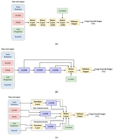
Figure 3.
Structures of the three NNs implemented in this study. (a) Dense NN, with 1,170,054 trainable parameters. Numbers in parenthesis represent layer node count. (b) Sequential NN, with 1,046,278 trainable parameters. (c) DgNN, with 1,018,094 trainable parameters.
In designing the third NN, interactions between the 12 different inputs (see Table 1) and their effect on crop growth were considered. Domain knowledge was incorporated into the NN by separating inputs into a branched structure based on their relationship to crop growth. TgML studies suggest that organizing NN inputs to reflect their real world interactions may improve performance [15]. For example, Khandelwal et al. [16] were able to improve overall streamflow prediction by 17% versus traditional LSTM architecture by training dedicated LSTM layers to predict intermediate variables, such as snow pack and soil water content. Although the dataset used in this study does not include target intermediate variables, it is possible to construct a NN structure that encourages LSTM hidden states to learn and track intermediate variables by separating the relevant inputs through a branched structure. For example, excess photoperiod during vegetative stages has been shown to delay crop progress, but increase leaf initiation rate [37,38], and excess solar radiation or photoperiod is used in mechanistic crop models to determine growth stage timing (e.g., [27]). In addition, soil moisture stress, due to low rainfall, in juvenile corn has been found to delay growth progression and reduce final plant size [39,40]. Typically, the effects of these two drivers on canopy growth and crop progress are modeled separately [27,41,42]. In this study, solar radiation and soil moisture-related inputs were separated from FPAR and AGDD using a LSTM-based branched structure, similar to their treatment within agronomic models, to encourage LSTM branches to learn and track these intermediate variables (Figure 3c).
Domain knowledge regarding timing and impact of different crop growth drivers during the growing season was incorporated using an attention mechanism. Attention in NNs allows a network to learn the importance of different inputs. Many natural language processing tasks involving LSTM utilize attention mechanisms to calculate the importance of different words in a sentence, e.g., [43,44]. In this study, self-attention based on Multi-Head Attention [45] is employed to allow the NN to learn importance weightings for different meteorological inputs. Agronomic literature suggests that surplus or deficit of solar radiation and rainfall during particular weeks in the growth cycle are what impact crop growth [37,40]. Attention mechanisms were added to both the solar radiation and soil moisture branches to exploit the time-dependent effects of solar radiation and rainfall as growth drivers in corn. The final branched structure with attention mechanisms is shown in Figure 3c. This NN is hereafter referred to as the Domain-guided NN (DgNN).
2.4. NN Loss, Validation and Evaluation
In this study, Kullback–Leibler Divergence () was used as the loss function for all NNs. is a measure of the difference between two probability distributions. is often used in NN regression problems with targets that are distributions. Given two distributions and , is calculated as:
Here is used as it provides a measure of the difference between the predicted and actual distributions of crop progress for a given week.
The 17-year CGSE dataset was split into 13 training years and 4 test years, and NN hyperparameters were selected using five-fold cross-validation on the training data. An initial 300 epochs were used in conjunction with early stopping, with a patience of 30 (i.e., 1/10th of the total) epochs and best weights restoration. Early stopping was determined based on NN loss on a single randomly selected year from the training data of each fold, kept separate and assessed at the end of each epoch. NNs were trained using the Adam optimizer with default parameters and a learning rate of 1 × 10⁻⁵. All NNs stopped early during training. In this study, the Dense NN followed a traditional funnel structure with layer widths ranging from 1024 to 128 nodes. Both the Sequential NN and DgNN used LSTM units with 64 hidden nodes and a 128 node dense layer. Dense and LSTM nodes used ReLU activation functions and layer weights were initialized using the GlorotUniform initializer. Dropout was used between hidden layers with a rate of 0.2. Each NN used a six head softmax output layer, with each head corresponding to one of the six growth stages defined in Section 2.1. For self-attention, a two-headed attention layer with a key dimension of 40 was used. All NNs were implemented using Python 3.9 and the Tensorflow-Keras python library [46].
As shown in Table 2 and Table 3, the four test years, 2009, 2012, 2014, and 2019 were chosen based upon deviation from the mean of the dataset in terms of rainfall, planting and harvest dates. All test years remained unseen by NNs during the design phase, and were only used for NN evaluation after selection of the final NN parameters. Initially during evaluation we trained the NNs using the average number of epochs required from early stopping during model validation, but reverted to the same early stopping technique used during NN validation, with the loss on a single randomly selected year (2004) monitored for all NNs. One instance of each NN structure was trained with time series inputs from all WOY in the training years, then produced estimates for every WOY in the test years.
Table 2.
State-wide deviations of precipitation and solar radiation during test years from 2003 to 2019 study period mean. Standard deviations are given in parenthesis.
Table 3.
State-wide deviations of crop progress during test years from the 2003–2019 study period mean. Values indicate time to cumulative progress into growth stage at 50%. Standard deviations are given in parenthesis.
For comparison to existing CGSE approaches, a Hidden Markov Model-based (HMM) CGSE method presented by Shen et al. was implemented [4]. This method uses a standard Expectation Maximization (EM) algorithm along with USDA CPRs to supply priors and transition matrices to the model. Following the method from [4], the HMM was run for 100 runs on the 13 training years, with a 4-year random subset from within the training years selected each run to act as validation data. Average performance over 100 runs was used to reduce EM sensitivity to initialization and local minima. During testing, the HMM was run 10 times on each of the four test years and the mean of these runs is the final performance reported.
ASD-level CGS estimates for the NNs and HMM were aggregated to state-level estimates for comparison via weighted sum, with ASD weights calculated based on the number of corn fields in each ASD that passed the processing criteria, explained in Section 2.1 and shown in Figure 2. Performance of the three NN structures and the HMM were evaluated against state-wide USDA CPRs using two metrics. The first, Nash–Sutcliffe efficiency (NSE), is a measure commonly used in hydrology and crop modeling to quantify how well a model describes an observed time series versus the mean value of that time series, and is defined as:
where is the model estimate at time t, is the observed value at time t, and is the mean value of the observed time series. NSE ranges from to a maximum of 1, where 1 means the model perfectly describes the observed time series. An NSE of below 0 means the model is worse at describing the observed time series than the observed time series mean. In this study, NSE is used as a metric for how well each NN estimates the percentage of corn in a given growth stage over time.
The second metric, cosine similarity (CS), is a measure of the angle between two vectors in a multi-dimension space. CS between two vectors and is calculated as:
In this study, CS is used as a metric for the accuracy of each NN in describing crop progress across all stages for a single week. CS ranges from −1 to +1, representing vectors that are exactly opposite in direction to exactly the same in direction. Orthogonal vectors have a CS of 0. A CS value of 1 means that the CGSE method produces perfect estimates of the amount of corn in each growth stage for that week. Lower CS values indicate higher discrepancies between estimated and real crop progress across all stages for that week.
2.5. Visualization of NN Operation
Uniformed Manifold Approximation and Projection (UMAP) [47] was used to visualize layer activations and gain insight into the differences in behavior among NN structures. UMAP is a dimension reduction technique that is often used for visualizing high-dimension data, e.g., [48]. For UMAP embedding, local neighborhoods of size 15 were used and hidden layer activations were embedded to 2 dimensions. Layer activations for training and test data were visualized for the layers in each NN feeding into the 128 node dense and softmax layers, these being common to all three NNs (see Figure 3). Color representations of crop progress were formed by reducing the six crop stages to three RGB channels using a UMAP reduction to 3 dimensions, with 15 neighbors.
3. Results
3.1. Model Validation
Table 4 shows the state-wide means and standard deviations of NSE for each of the five CGS for five-fold cross-validation on the training data. Overall, the three NN structures performed better than the HMM. The HMM had particularly low NSE during Silking and Mature stages, meaning those stages were difficult to estimate. Figure 4 shows five-fold cross-validated CS performance on the training data, with box plots representing the minimum, maximum, and inter-quartile range of the CS. Week-to-week CS for the HMM was also significantly worse than for the NNs. It should be noted that the CS scale for the HMM plot is larger (0.2 to 1) than those used for the NNs in Figure 4. Among the three NN structures, the Dense NN performed the worst, with the lowest NSE for all stages except Grainfill. In addition, the range of CS values is larger for the Dense NN during transition between Silking and Grainfill (WOY 32-33) and Mature to Harvest (WOY 42-43).
Table 4.
Mean state-wide NSEs and their standard deviations for five-fold cross validation on the 13-year training data. Standard deviations are given in parenthesis. Bold numbers represent highest NSE and lowest standard deviation.
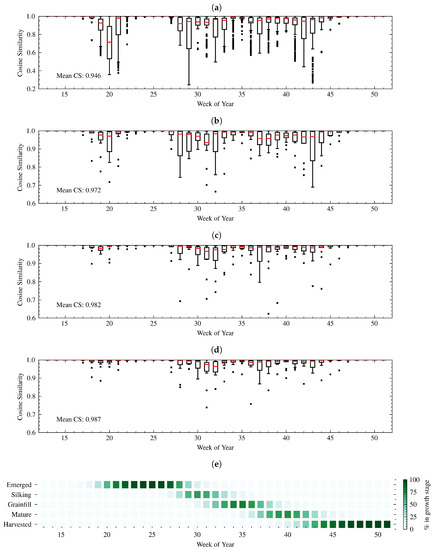
Figure 4.
Week-to-week state-wide CS between real and estimated crop progress of (a) HMM (b) Dense NN (c) Sequential NN (d) DgNN for five-fold cross validation on the 13-year training data. Box plots are mean (red) and inter-quartile range (IQR) and whiskers are 1.5 × IQR. Outliers are plotted as single points. (e) Average crop progress from USDA crop progress reports during the training years. Scales for HMM (1 to 0.2) and the NNs (1 to 0.6) are different to allow inclusion of all HMM points.
The Sequential NN improved upon the Dense NN cross-validated NSEs, particularly for the Mature stage. NSE for both the Emerged and Harvested stages for the Sequential NN were also very similar to the DgNN model during validation. Mean CS was only slightly lower for the Sequential NN than for the DgNN, and the range of CS values over the training data is actually higher during the start of Grainfill (WOY 31). During cross-validation, CGSE proved more challenging for the Silking, Grainfill, and Mature stages. Cross-validated CS performance was high for all methods for weeks 22–27, during the height of the Emerged stage. This is because the Emerged stage is the longest in-season stage, and as such, at certain weeks, such as WOY 25, the crop is 100% emerged for all years during the study period. Similarly, CS performance was high for all methods after WOY 45, after which nearly 100% of the crop had reached the Harvested stage in all training years.
3.2. Model Evaluation
The four test years used for evaluation were 2009, 2012, 2014, and 2019. In 2009, planting was delayed by heavy rains in May and a cool July (6 °C below normal) delayed crop progress. Rain at the end of September and through much of October delayed harvest significantly [49]. For 2012, corn planting began quickly, but was slowed by rain in May. Low rainfall and hot temperatures in June and July caused both soil moisture deficit and fast crop progress. A dry and warm late August and early September brought about early crop maturity and harvesting began early [50]. Crops progression in 2014 was similar to the 17-year study period average. Planting was slightly behind average during April, but by mid-July corn progression had surpassed the study period average. Wet fields and high grain moisture slowed harvest progress in October [51]. In 2019, rain in April and May delayed corn planting progress, and by the end of a drier June corn emergence was over a week behind average. Cooler temperatures in September also slowed crop progress, leading to delayed crop maturity and harvesting [52].
Table 5 shows state-wide means and standard deviations of NSE performance for the four test years. The HMM showed lower NSEs during test years for all stages except the Emerged stage. The HMM Mature NSE was significantly lower than in cross-validation, with an average less than 0.3 and standard deviation greater than 0.4. The Dense NN had higher NSEs than the HMM for the four test years, but also a lower mean and higher standard deviation than its cross-validated performance. The Sequential NN produced higher mean and lower standard deviation NSEs than the Dense NN in each stage, and also produced the best NSE for the Silking stage of any method. The DgNN produced the best mean NSE results on the test data for all stages except Silking, with significantly higher performance for the Mature stage. Like all methods, it produced lower mean NSEs than its cross-validated performance on the training data; however, it also produced a lower standard deviation for Grainfill performance on the test years.
Table 5.
Mean state-wide NSEs and their standard deviations for the four test years. Standard deviations are given in parenthesis. Bold numbers represent highest NSE and lowest standard deviation.
Figure 5, Figure 6, Figure 7 and Figure 8 show the CS for the four test years. Dense NN CS values for the test years, particularly 2009 (Figure 5) and 2012 (Figure 6), were lower than the range produced during cross-validation. While the Sequential NN was able to produce more accurate overall estimates of all-stage crop progress (as measured by CS) during some of the most difficult periods for all models, it also suffered greater CS performance degradation than the other NNs during some CGS transition periods. The DgNN maintained the highest CS for some of the most difficult periods, such as the Grainfill–Mature–Harvested transitions, during the test years for all NNs. The DgNN was also less prone to CS performance drops during the start and end of the Emergence stage, which were particularly pronounced for the other models in 2009 (WOY 29–30) and 2014 (WOY 18–19). In addition, as seen in Table 6, the DgNN produced the best estimates across all growth stages for the greatest number of weeks in each of the test years, producing the highest CS value for 39% more weeks than the next best NN.
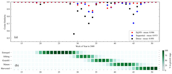
Figure 5.
(a) Week-to-week CS between actual and estimated crop progress for the NNs in 2009; and (b) actual crop progress for 2009 is shown below.
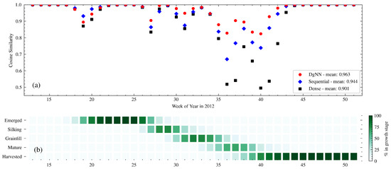
Figure 6.
(a) Week-to-week CS between actual and estimated crop progress for the NNs in 2012; and (b) actual crop progress for 2012 is shown below.
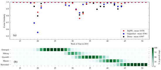
Figure 7.
(a) Week-to-week CS between actual and estimated crop progress for the NNs in 2014; and (b) actual crop progress for 2014 is shown below.
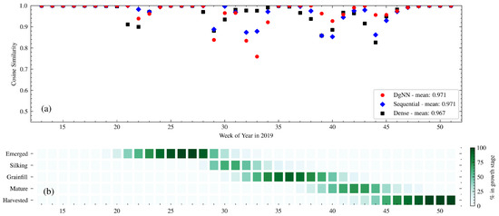
Figure 8.
(a) Week-to-week CS between actual and estimated crop progress for the NNs in 2019; and (b) actual crop progress for 2019 is shown below.
Table 6.
Total number of weeks during test years that each NN produced the highest CS value that week. Count includes each NN (one or more) that produced the highest CS value. Bold numbers represent highest number of weeks.
Table 7 shows NSE performance for each of the test years. For the 2009 test year, the DgNN outperformed all other models, with the highest NSE for all stages except Emerged. Similar to what was seen during model validation, all NNs had reduced performance during the stages where corn transitioned into and out of Silking (see Figure 5). The Dense NN showed greater performance degradation than the LSTM-based NNs during this period, with significantly lower CS from WOY 29–34. There was a decrease in CS due to a delayed harvest around WOY 45, a time when close to 100% of the crop had been harvested for every year represented in the training data. The Sequential NN was the worst affected. The DgNN, however, suffered very little decrease in CS during that week. Figure 9 shows cumulative crop progress for each stage for each of the years. During 2009, each of the three NNs was early in estimating progress for every stage except Emerged.
Table 7.
State-wide NSEs for each of the four test years. Bold numbers represent highest NSE.
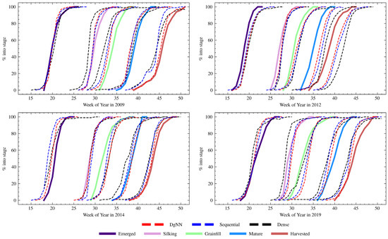
Figure 9.
State-wide estimated cumulative crop progress of each NN (dashed) for the four test years compared to actual cumulative crop progress (solid).
The year 2012 produced the worst NSE across all models for the Grainfill and Mature stages. This is expected, given the large deviation in crop progress timing from the study mean during that year (see Table 3). With the exception of the Emerged stage, the DgNN best described each of the growth stages, as measured by NSE. The week-to-week CS performance degraded less for the DgNN than the other NNs during the fast-moving WOY 33–43 Grainfill-Mature progression, as seen in Figure 6. The pronounced problems of all NNs during this period may have been caused by the weather-induced fast crop progression and sustained drought during the 2012 growing season. Significant soil moisture stress contributed to degradation in corn crop condition [53], which may have affected canopy appearance and the FPAR signal. In addition, warm temperatures during the growing season sped up crop progress to rates not seen since 1987 [50]. As shown in Table 3, growth stage time to 50% was over two standard deviations less the mean for both Mature and Harvested stages. This is in contrast with 2009, where a delay of comparable magnitude (+20 days) did not have as significant an effect on later season week-to-week performance. There were significant delays in NN progress estimation for Mature and Harvested in 2012, as show in Figure 9.
In 2014, Silking NSE for the NNs was low, even though crop progress that year was relative typical of the study period. All three NN structures were late in estimating the onset of the Grainfill stage, as shown in Figure 9 and also reflected in the decline in CS between WOY 30 and 34 (see Figure 7). Cumulative progress estimates, as seen in Figure 9, exhibit the closest cumulative estimation curves for Silking of any of the test years, particularly with the DgNN. However, because the NNs were late in predicting the onset of Grainfill, NSE performance for Silking degraded. Whereas here the NNs performed well at estimating crop progress into Silking, they could not accurately describe the rate at which the crop progressed out of that stage. NNs were also early in estimating emergence, which degraded CS during WOY 18–21.
NN performance for Silking also suffered in 2019, with low Silking NSE caused by late DgNN and Sequentiall NN estimates for the start of the Grainfill stage, a problem not experienced by the Dense NN (see Figure 9). The opposite is true for the Mature stage, where NSE is higher for the DgNN than the other two NNs. This is reflected in the week-to-week CS values for WOY 37–46 (see Figure 8), higher for the DgNN, during which time the crop was transitioning from Grainfill to Mature to Harvested.
A common theme for all CGSE methods across all training and test years is the three periods of easy estimation that happen at different times during the growing season: WOY 13–17, when crops have yet to emerge, periods around WOY 25 (100% Emerged for all study years), and WOY 48–51 when the vast majority of the crop has been harvested. Predictably, the most difficult periods for estimation as measured by CS are those with the crop in two or more stages, and progress of mid-season stages proved more difficult to estimate than start- and end-of-season stages. Silking is the shortest yet most critical growth stage in terms of potential yield loss, but was the most difficult to estimate for all NNs. Compared to the Emerged and Harvested stages, where significant FPAR gradients help to highlight timing, canopy appearance and therefore FPAR remain relatively unchanged during the Silking–Grainfill transition. Estimation of the this transition was a consistent problem. With the exception of 2009, when the Grainfill stage was delayed by 11 days compared to the study period average, all NNs were late in their estimations of the cumulative progress into the Grainfill stage (see Figure 9). In the absence of measurable canopy change, AGDD is a useful proxy for estimating progress from Silking to Grainfill. AGDD, however, is cultivar specific, and cultivars are selected based on different factors, such as planting timing and drought risk. Cultivar-specific variation in required AGDD for progress through Silking and the short duration of that stage may reduce the effectiveness of AGDD as a proxy. In addition, AGDD for this study is accumulated from April 8th of each year and so, due to variable inter-year planting dates, is not an exact measure of how much AGDD that year’s crop has accumulated. As the NNs presented here have provided accurate estimates of the timing of progression into Silking, one possible improvement for future methods could be to use weekly GDD as an input so that the NN could learn the accumulation of GDD required relative to the start of Silking. On the other hand, AGDD provides a measure of accumulated temperature over the growing season that serves as an anchor for plausible crop progression. There is no guarantee than NNs presented with GDD only would be able to effectively learn variable accumulation functions that, un-guided, lead to better estimates.
All NN structures produced NSE and CS results that were worse during model evaluation. This suggests that each of the methods experienced overfitting. In any NN implementation for RS, some overfitting is expected because of the limited number of years of data available for RS-based methods. This leaves CGSE approaches vulnerable to test years with progress timing that is under-represented in the training data. This problem is particularly pronounced in 2012, where fast crop progression saw corn begin to mature in WOY 34, two weeks before any year in the training set. This fast crop progress, however, degraded the performance of the LSTM-based methods less than the HMM and the Dense NN, suggesting that the ability of LSTM to handle variable length gaps between key events make these methods more robust to outlier years such as 2012. Further studies could investigate the relationship between CGSE NN complexity and overfitting through an a posteriori ablation study, e.g., [54].
One notable area of performance degradation were the low NSEs in the DgNN implementation for Silking during model evaluation. In the DgNN structure, self-attention is used to take advantage of field studies in agronomy. In this context, there is one caveat to using attention that may cause overfitting. Since zero-padded, variable length time series were used, the majority of time series inputs in the training-set have later season values set to zero. Therefore, there are less examples of non-zero values during later weeks and the attention layers may tend to reduce the assigned importance of later inputs, introducing a bias. For example, two thirds of all time series in this study have the last one third of their input tensor zero-padded. This could affect the ability of the DgNN to identify important differences later in the season.
Overall, the DgNN showed significant improvement in estimating CGS over the HMM and the other two NNs, particularly in Mature stage NSE and in CS for weeks with multiple overlapping stages. However, the DgNN had reduced NSE for Silking during evaluation due to difficulty in estimating the timing of the Silking–Grainfill transition. Given the higher Silking NSE of the Sequential NN during evaluation, future studies may be able to combine the strengths of both NNs through ensemble methods such as boosting (e.g., [55]) or estimation averaging (e.g., [56]).
3.3. UMAP Visualization of Layer Activations
Figure 10 and Figure 11 show layer activations for the final layers of each NN preceding their respective 128 node and softmax layers. Layer activations have been reduced using UMAP and labeled stages in the colorbar represent the height of each new stage. Figure 10 illustrates how the LSTM-based NNs treat the time series differently from the Dense NN. Each of the separate branches visible in the activation space for both the DgNN and Sequential NN contain time series from a specific ASD. The Dense NN, however, does not keep time series from different ASDs as separate, even though it is given the same location information. This may be a source of performance boost for the LSTM-based models, as test year data is projected into the activation space closer to other data from the same ASD. Regression performed by final layers to estimate crop progress is then more strongly influenced by training time series from the same region. This is a benefit as farmers in different ASDs elect to plant cultivars with traits more suited to the local climate. As such, regression performed in an activation space that keeps different ASDs more separate may be more robust to inter-season variation.
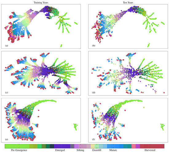
Figure 10.
UMAP visualizations of combined activations from layers feeding into the 128 node layer for training and test years for (a,b) Dense NN; (c,d) Sequential NN; (e,f) DgNN.
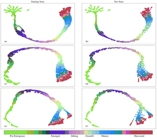
Figure 11.
UMAP visualizations of 128 node layer activations feeding into the softmax layer for training and test years for (a,b) Dense NN; (c,d) Sequential NN; (e,f) DgNN.
The UMAP plots also show evidence of NN overfitting, manifest as noisier delineation among clusters in the test data. For the Dense NN, this is most observable in the Pre-Emergence to Emerged green to purple (Figure 11a,b), and the Mature to Harvested transitions between blue and maroon (Figure 10a,b). While the above is a simple analysis of layer activations using UMAP for model evaluation purposes, UMAP visualizations may be used as a diagnostic tool in future work to assess the impact of including different structures and mechanisms during CGSE NN design.
4. Conclusions
In this study, an agronomy-informed neural network, DgNN, was developed to provide in-season CGSE estimates. The DgNN separates inputs that can be treated as independent crop growth drivers using a branched structure, and uses attention mechanisms to account for the varying importance of inputs during the growing season. The DgNN was trained and evaluated on RS and USDA CPR data for Iowa from 2003 to 2019 using NSE and CS as metrics. The DgNN structure was compared to a HMM and two NN structures of similar complexity. The DgNN outperformed each of the other methods on all growth stages for five-fold cross validation on the training data, with an average improvement in NSE across all stages of 22% versus the HMM and 2.2% versus the next best NN. The four models were evaluated on four test years that remained unseen during validation. The mean performance during model evaluation was also higher for the DgNN than the other NNs and the HMM. Mean evaluation NSE for the DgNN across all stages was 43% versus the HMM and 4.0% higher versus the next best NN (5.9% when excluding Silking). The DgNN also had 39% more weeks with the highest CS across all test years than the next best NN. CS metrics showed that weeks when a region’s crop is in multiple stages concurrently are more difficult to estimate. Estimating timing of the short yet critical growth stage of Silking was the most difficult for all methods, particularly the Silking-to-Grainfill stage transition. During evaluation, Silking NSE for the DgNN was reduced primarily due to the DgNN’s inability to correctly estimate the timing of this transition. While performance of all methods was lower on the test data, LSTM-based methods, the DgNN and Sequential NN, were found to be more robust when presented with abnormal crop progress during model evaluation. UMAP analysis of hidden layers indicated that LSTM-based NNs hold time series from different locations more separate in the activation space.
This study demonstrated that a domain-guided design, such as the DgNN, can improve in-season CGSE compared to NN structures of equivalent complexity. However, UMAP-based NN structure diagnostics and ablation studies to investigate optimum NN complexity may be able to further improve upon these results. In addition, ensemble methods may also address stage-specific shortcomings, such as Silking–Grainfill transition. The DgNN in this study was specifically tailored to CGSE for corn. The approach can easily be extended to other crops by integrating agronomic knowledge of their growth drivers into similar network design.
Author Contributions
Conceptualization, all authors; methodology, all authors; validation, G.W.; investigation, all authors; writing—original draft preparation, G.W.; writing—review and editing, all authors; visualization, G.W. All authors have read and agreed to the published version of the manuscript.
Funding
This research was supported by funding from the NASA Terrestrial Hydrology Program (Grant No. NNX16AQ24G).
Data Availability Statement
Publicly available datasets used in this study can be found at citations in Table 1. USDA crop progress data for Iowa was obtained from the USDA-NASS Upper Midwest Regional Office.
Acknowledgments
The authors would like to thank the USDA-NASS Upper Midwest Regional Office for providing the tabulated ASD level crop progress data for this study.
Conflicts of Interest
The authors declare no conflict of interest.
References
- Ray, D.K.; Gerber, J.S.; MacDonald, G.K.; West, P.C. Climate variation explains a third of global crop yield variability. Nat. Commun. 2015, 6, 5989. [Google Scholar] [CrossRef] [PubMed] [Green Version]
- Iizumi, T.; Ramankutty, N. Changes in yield variability of major crops for 1981–2010 explained by climate change. Environ. Res. Lett. 2016, 11, 034003. [Google Scholar] [CrossRef]
- Mehrabi, Z.; Ramankutty, N. Synchronized failure of global crop production. Nat. Ecol. Evol. 2019, 3, 780–786. [Google Scholar] [CrossRef] [Green Version]
- Shen, Y.; Wu, L.; Di, L.; Yu, G.; Tang, H.; Yu, G.; Shao, Y. Hidden Markov Models for Real-Time Estimation of Corn Progress Stages Using MODIS and Meteorological Data. Remote Sens. 2013, 5, 1734–1753. [Google Scholar] [CrossRef] [Green Version]
- Zeng, L.; Wardlow, B.D.; Wang, R.; Shan, J.; Tadesse, T.; Hayes, M.J.; Li, D. A hybrid approach for detecting corn and soybean phenology with time-series MODIS data. Remote Sens. Environ. 2016, 181, 237–250. [Google Scholar] [CrossRef]
- Seo, B.; Lee, J.; Lee, K.D.; Hong, S.; Kang, S. Improving remotely-sensed crop monitoring by NDVI-based crop phenology estimators for corn and soybeans in Iowa and Illinois, USA. Field Crops Res. 2019, 238, 113–128. [Google Scholar] [CrossRef]
- Diao, C. Remote sensing phenological monitoring framework to characterize corn and soybean physiological growing stages. Remote Sens. Environ. 2020, 248, 111960. [Google Scholar] [CrossRef]
- Ghamghami, M.; Ghahreman, N.; Irannejad, P.; Pezeshk, H. A parametric empirical Bayes (PEB) approach for estimating maize progress percentage at field scale. Agric. For. Meteorol. 2020, 281, 107829. [Google Scholar] [CrossRef]
- Orynbaikyzy, A.; Gessner, U.; Conrad, C. Crop type classification using a combination of optical and radar remote sensing data: A review. Int. J. Remote Sens. 2019, 40, 6553–6595. [Google Scholar] [CrossRef]
- Jia, X.; Khandelwal, A.; Mulla, D.J.; Pardey, P.G.; Kumar, V. Bringing automated, remote-sensed, machine learning methods to monitoring crop landscapes at scale. Agric. Econ. 2019, 50, 41–50. [Google Scholar] [CrossRef]
- Kerner, H.; Sahajpal, R.; Skakun, S.; Becker-Reshef, I.; Barker, B.; Hosseini, M.; Puricelli, E.; Gray, P. Resilient In-Season Crop Type Classification in Multispectral Satellite Observations using Growth Stage Normalization. arXiv 2020, arXiv:2009.10189. [Google Scholar]
- Teimouri, N.; Dyrmann, M.; Jørgensen, R.N. A Novel Spatio-Temporal FCN-LSTM Network for Recognizing Various Crop Types Using Multi-Temporal Radar Images. Remote Sens. 2019, 11, 990. [Google Scholar] [CrossRef] [Green Version]
- Weiss, M.; Jacob, F.; Duveiller, G. Remote sensing for agricultural applications: A meta-review. Remote Sens. Environ. 2020, 236, 111402. [Google Scholar] [CrossRef]
- USDA National Agricultural Statistics Service Cropland Data Layer. 2008–2019. Type: Dataset. Available online: http://nassgeodata.gmu.edu/CropScape/ (accessed on 5 November 2020).
- Karpatne, A.; Atluri, G.; Faghmous, J.H.; Steinbach, M.; Banerjee, A.; Ganguly, A.; Shekhar, S.; Samatova, N.; Kumar, V. Theory-Guided Data Science: A New Paradigm for Scientific Discovery from Data. IEEE Trans. Knowl. Data Eng. 2017, 29, 2318–2331. [Google Scholar] [CrossRef]
- Khandelwal, A.; Xu, S.; Li, X.; Jia, X.; Stienbach, M.; Duffy, C.; Nieber, J.; Kumar, V. Physics Guided Machine Learning Methods for Hydrology. arXiv 2020, arXiv:2012.02854. [Google Scholar]
- Willard, J.; Jia, X.; Xu, S.; Steinbach, M.; Kumar, V. Integrating Physics-Based Modeling with Machine Learning: A Survey. arXiv 2020, arXiv:2003.04919. [Google Scholar]
- Karpatne, A.; Watkins, W.; Read, J.; Kumar, V. Physics-guided Neural Networks (PGNN): An Application in Lake Temperature Modeling. arXiv 2018, arXiv:1710.11431. [Google Scholar]
- Hu, X.; Hu, H.; Verma, S.; Zhang, Z.L. Physics-Guided Deep Neural Networks for Power Flow Analysis. IEEE Trans. Power Syst. 2020, 36, 2082–2092. [Google Scholar] [CrossRef]
- Shahhosseini, M.; Hu, G.; Huber, I.; Archontoulis, S.V. Coupling machine learning and crop modeling improves crop yield prediction in the US Corn Belt. Sci. Rep. 2021, 11, 1606. [Google Scholar] [CrossRef] [PubMed]
- Chen, T.S.; Aoike, T.; Yamasaki, M.; Kajiya-Kanegae, H.; Iwata, H. Predicting rice heading date using an integrated approach combining a machine learning method and a crop growth model. Front. Genet. 2020, 11, 1643. [Google Scholar] [CrossRef] [PubMed]
- Rong, M.; Zhang, D.; Wang, N. A Lagrangian Dual-based Theory-guided Deep Neural Network. arXiv 2020, arXiv:2008.10159. [Google Scholar]
- Wang, N.; Zhang, D.; Chang, H.; Li, H. Deep learning of subsurface flow via theory-guided neural network. J. Hydrol. 2020, 584, 124700. [Google Scholar] [CrossRef] [Green Version]
- USDA National Agricultural Statistics Service. World Agricultural Production; Technical Report WAP 4-21; USDA Foreign Agricultural Service: Washington, DC, USA, 2021. [Google Scholar]
- USDA National Agricultural Statistics Service. NASS—Quick Stats. 2017: Corn—Acres Planted. Type: Dataset. Available online: https://data.nal.usda.gov/dataset/nass-quick-stats (accessed on 15 March 2021).
- Wang, S.; Di Tommaso, S.; Deines, J.M.; Lobell, D.B. Mapping twenty years of corn and soybean across the US Midwest using the Landsat archive. Sci. Data 2020, 7, 307. [Google Scholar] [CrossRef]
- Lizaso, J.I.; Boote, K.J.; Jones, J.W.; Porter, C.H.; Echarte, L.; Westgate, M.E.; Sonohat, G. CSM-IXIM: A New Maize Simulation Model for DSSAT Version 4.5. Agron. J. 2011, 103, 766–779. [Google Scholar] [CrossRef]
- Kiniry, J.R. Maize Phasic Development. In Agronomy Monographs; Hanks, J., Ritchie, J.T., Eds.; American Society of Agronomy, Crop Science Society of America, Soil Science Society of America: Madison, WI, USA, 2015; pp. 55–70. [Google Scholar] [CrossRef]
- Thornton, M.; Shrestha, R.; Wei, Y.; Thornton, P.; Kao, S.; Wilson, B. Daymet: Daily Surface Weather Data on a 1-km Grid for North America, Version 4; ORNL Distributed Active Archive Center: Oak Ridge, TN, USA, 2020. [Google Scholar] [CrossRef]
- Myneni, Y.R.; Knyazikhin, T.P. MCD15A3H MODIS/Terra+Aqua Leaf Area Index/FPAR 4-day L4 Global 500m SIN Grid V006. NASA EOSDIS Land Processes DAAC. 2015. Available online: https://lpdaac.usgs.gov/products/mcd15a3hv006/ (accessed on 5 November 2020).
- Staff, S.S. Gridded Soil Survey Geographic (gSSURGO) Database for the United States of America and the Territories, Commonwealths, and Island Nations served by the USDA-NRCS; Technical Report; USDA National Resource Conversvation Service: Washington, DC, USA, 2020. [Google Scholar]
- Chen, J.; Jönsson, P.; Tamura, M.; Gu, Z.; Matsushita, B.; Eklundh, L. A simple method for reconstructing a high-quality NDVI time-series data set based on the Savitzky–Golay filter. Remote Sens. Environ. 2004, 91, 332–344. [Google Scholar] [CrossRef]
- Hochreiter, S.; Schmidhuber, J. Long Short-Term Memory. Neural Comput. 1997, 9, 1735–1780. [Google Scholar] [CrossRef] [PubMed]
- Yu, Y.; Si, X.; Hu, C.; Zhang, J. A Review of Recurrent Neural Networks: LSTM Cells and Network Architectures. Neural Comput. 2019, 31, 1235–1270. [Google Scholar] [CrossRef]
- Khaki, S.; Wang, L.; Archontoulis, S.V. A CNN-RNN Framework for Crop Yield Prediction. Front. Plant Sci. 2020, 10, 1750. [Google Scholar] [CrossRef] [PubMed]
- Graves, A. Long short-term memory. In Supervised Sequence Labelling with Recurrent Neural Networks; Springer: Berlin/Heidelberg, Germany, 2012; pp. 37–45. [Google Scholar]
- Warrington, I.J.; Kanemasu, E.T. Corn Growth Response to Temperature and Photoperiod I. Seedling Emergence, Tassel Initiation, and Anthesis. Agron. J. 1983, 75, 749–754. [Google Scholar] [CrossRef]
- Warrington, I.J.; Kanemasu, E.T. Corn Growth Response to Temperature and Photoperiod II. Leaf-Initiation and Leaf-Appearance Rates. Agron. J. 1983, 75, 755–761. [Google Scholar] [CrossRef]
- NeSmith, D.; Ritchie, J. Short- and Long-Term Responses of Corn to a Pre-Anthesis Soil Water Deficit. Agron. J. 1992, 84, 107–113. [Google Scholar] [CrossRef]
- Çakir, R. Effect of water stress at different development stages on vegetative and reproductive growth of corn. Field Crops Res. 2004, 89, 1–16. [Google Scholar] [CrossRef]
- Jones, C.; Ritchie, J.; Kiniry, J.; Godwin, D.; Otter, S. The CERES wheat and maize models. In Proceedings of the International Symposium on Minimum Data Sets for Agrotechnology Transfer, ICRISAT Center, Patancheru, India, 21–26 March 1983; pp. 95–100. [Google Scholar]
- Holzworth, D.P.; Huth, N.I.; deVoil, P.G.; Zurcher, E.J.; Herrmann, N.I.; McLean, G.; Chenu, K.; van Oosterom, E.J.; Snow, V.; Murphy, C.; et al. APSIM–Evolution towards a new generation of agricultural systems simulation. Environ. Model. Softw. 2014, 62, 327–350. [Google Scholar] [CrossRef]
- Young, T.; Hazarika, D.; Poria, S.; Cambria, E. Recent Trends in Deep Learning Based Natural Language Processing. IEEE Comput. Intell. Mag. 2018, 13, 55–75. [Google Scholar] [CrossRef]
- Liu, Y.; Sun, C.; Lin, L.; Wang, X. Learning Natural Language Inference using Bidirectional LSTM model and Inner-Attention. arXiv 2016, arXiv:1605.09090. [Google Scholar]
- Vaswani, A.; Shazeer, N.; Parmar, N.; Uszkoreit, J.; Jones, L.; Gomez, A.N.; Kaiser, L.; Polosukhin, I. Attention Is All You Need. arXiv 2017, arXiv:1706.03762. [Google Scholar]
- Abadi, M.; Barham, P.; Chen, J.; Chen, Z.; Davis, A.; Dean, J.; Devin, M.; Ghemawat, S.; Irving, G.; Isard, M.; et al. Tensorflow: A system for large-scale machine learning. In Proceedings of the 12th {USENIX} symposium on operating systems design and implementation ({OSDI} 16), Savannah, GA, USA, 2–4 November 2016; pp. 265–283. [Google Scholar]
- McInnes, L.; Healy, J.; Melville, J. UMAP: Uniform Manifold Approximation and Projection for Dimension Reduction. arXiv 2020, arXiv:1802.03426. [Google Scholar]
- Becht, E.; McInnes, L.; Healy, J.; Dutertre, C.A.; Kwok, I.W.H.; Ng, L.G.; Ginhoux, F.; Newell, E.W. Dimensionality reduction for visualizing single-cell data using UMAP. Nat. Biotechnol. 2019, 37, 38–44. [Google Scholar] [CrossRef] [PubMed]
- USDA-National Agricultural Statistics Service Upper Midwest Region, Iowa Field Office. 2010 Iowa Agricultural Statistics; Technical Report; USDA: Washington, DC, USA, 2010. [Google Scholar]
- USDA-National Agricultural Statistics Service Upper Midwest Region, Iowa Field Office. 2013 Iowa Agricultural Statistics; Technical Report; USDA: Washington, DC, USA, 2013. [Google Scholar]
- USDA-National Agricultural Statistics Service Upper Midwest Region, Iowa Field Office. 2015 Iowa Agricultural Statistics; Technical Report; USDA: Washington, DC, USA, 2015. [Google Scholar]
- USDA-National Agricultural Statistics Service Upper Midwest Region, Iowa Field Office. 2020 Iowa Agricultural Statistics; Technical Report; USDA: Washington, DC, USA, 2020. [Google Scholar]
- USDA National Agricultural Statistics Service. NASS—Quick Stats. 2017: Corn—Crop Condition. Type: Dataset. Available online: https://data.nal.usda.gov/dataset/nass-quick-stats (accessed on 15 March 2021).
- Meyes, R.; Lu, M.; de Puiseau, C.W.; Meisen, T. Ablation Studies in Artificial Neural Networks. arXiv 2019, arXiv:1901.08644. [Google Scholar]
- Peerlinck, A.; Sheppard, J.; Senecal, J. AdaBoost with Neural Networks for Yield and Protein Prediction in Precision Agriculture. In Proceedings of the 2019 International Joint Conference on Neural Networks (IJCNN), Budapest, Hungary, 14–19 July 2019; IEEE: Budapest, Hungary, 2019; pp. 1–8. [Google Scholar] [CrossRef]
- Kussul, N.; Lavreniuk, M.; Shelestov, A.; Yailymov, B. Along the season crop classification in Ukraine based on time series of optical and SAR images using ensemble of neural network classifiers. In Proceedings of the 2016 IEEE International Geoscience and Remote Sensing Symposium (IGARSS), Beijing, China, 10–15 July 2016; IEEE: New York, NY, USA, 2016; pp. 7145–7148. [Google Scholar]
Publisher’s Note: MDPI stays neutral with regard to jurisdictional claims in published maps and institutional affiliations. |
© 2021 by the authors. Licensee MDPI, Basel, Switzerland. This article is an open access article distributed under the terms and conditions of the Creative Commons Attribution (CC BY) license (https://creativecommons.org/licenses/by/4.0/).