Technical Note

L-Band SAR Co-Polarized Phase Difference Modeling for Corn Fields

by
Matías Ernesto Barber
1,2,*,
David Sebastián Rava
1 and
Carlos López-Martínez
3
1
Quantitative Remote Sensing Group, Institute of Astronomy and Space Physics (IAFE), Buenos Aires 1428, Argentina
2
Department of Physics, Engineering School, University of Buenos Aires (UBA), Buenos Aires 1428, Argentina
3
Signal Theory and Communications Department (TSC), Universitat Politècnica de Catalunya (UPC), 08034 Barcelona, Spain
*
Author to whom correspondence should be addressed.
Remote Sens. 2021, 13(22), 4593; https://doi.org/10.3390/rs13224593
Submission received: 29 August 2021 / Revised: 9 November 2021 / Accepted: 11 November 2021 / Published: 15 November 2021
(This article belongs to the Special Issue ALOS-2/PALSAR-2 Calibration, Validation, Science and Applications)

Abstract

:
This research aims at modeling the microwave backscatter of corn fields by coupling an incoherent, interaction-based scattering model with a semi-empirical bulk vegetation dielectric model. The scattering model is fitted to co-polarized phase difference measurements over several corn fields imaged with fully polarimetric synthetic aperture radar (SAR) images with incidence angles ranging from 20° to 60°. The dataset comprised two field campaigns, one over Canada with the Uninhabited Aerial Vehicle Synthetic Aperture Radar (UAVSAR, 1.258 GHz) and the other one over Argentina with Advanced Land Observing Satellite 2 (ALOS-2) Phased Array type L-band Synthetic Aperture Radar (PALSAR-2) (ALOS-2/PALSAR-2, 1.236 GHz), totaling 60 data measurements over 28 grown corn fields at peak biomass with stalk gravimetric moisture larger than 0.8 g/g. Co-polarized phase differences were computed using a maximum likelihood estimation technique from each field’s measured speckled sample histograms. After minimizing the difference between the model and data measurements for varying incidence angles by a nonlinear least-squares fitting, well agreement was found with a root mean squared error of 24.3° for co-polarized phase difference measurements in the range of −170.3° to −19.13°. Model parameterization by stalk gravimetric moisture instead of its complex dielectric constant is also addressed. Further validation was undertaken for the UAVSAR dataset on earlier corn stages, where overall sensitivity to stalk height, stalk gravimetric moisture, and stalk area density agreed with ground data, with the sensitivity to stalk diameter being the weakest. This study provides a new perspective on the use of co-polarized phase differences in retrieving corn stalk features through inverse modeling techniques from space.

Graphical Abstract

1. Introduction

The potential of active microwaves to monitor agricultural areas is recognized as a key feature for supporting application-oriented approaches such as crop classification schemes (e.g., [1,2,3]), crop height estimation (e.g., [4,5,6]), soil moisture estimation (e.g., [7,8]), among others, and to aid decision-makers in managing and assessing agricultural resources. Towards this goal, the NASA/JPL’s UAVSAR airborne L-band mission was deployed to support several soil moisture and vegetation features inversion strategies [9,10,11]. In this respect, the systematic use of polarimetric SAR data from orbiting sensors at L-band over croplands was almost limited to JAXA’s Advanced Land Observing Satellite 2 (ALOS-2) Phased Array type L-band Synthetic Aperture Radar (PALSAR-2) mission (global.jaxa.jp/projects/sat/alos2) over the years. However, this situation has recently improved with the successful launch of the Argentinean L-band SAR constellation mission SAOCOM-1A and 1B (saocom.invap.com.ar) on 7 October 2018, and 30 August 2020, respectively. Both sensors have a lifespan of 5.5 years and were designed with interferometric and polarimetric capabilities. Within its goals, the SAOCOM constellation will provide fully polarimetric acquisitions dedicated to monitoring large cropland areas in Argentina, representing an important contribution to agriculture and hydrology worldwide.
The NASA-ISRO Synthetic Aperture Radar (NISAR) mission, which is planned to be launched in 2023, will provide L- and S-band full-polarized data over vegetated terrain, adding up its polarimetric capabilities to existing imagery [12]. In addition, the European Space Agency has recently signed the contract to develop the new high-priority Copernicus Radar Observation System for Europe in L-band (ROSE-L) as part of Europe’s Copernicus program. With a launch planned in 2028, this system will present polarimetric capabilities and its main product types and formats will be aligned as much as possible with the ones of Sentinel-1, for enhanced continuity [13].
Among major crops, corn is the most cultivated cereal worldwide according to the latest Food and Agriculture Organization (FAO) data [14], with a total production of 1149 Mt in 2019, followed by wheat (765.8 Mt), paddy rice (755.5 Mt), soybeans (333.7 Mt), and barley (159.0 Mt) in the same year. Following the significant SAR missions mentioned, amplitude and phase measurements will be systematically delivered to cover most of these major crops, among which corn fields have unique features: corn plants have the largest dimensions with stalk heights up to 3 m , stalk diameters up to 2.5 cm and large moisture contents up to 0.90 g / g [11,15,16]. Furthermore, corn seeds are usually planted in a regular pattern of 7 to 9 plants per square meter onto rows separated 75 cm apart [11,16,17]. This pattern and the unique plant features, often in the resonant regime for wavelengths at the L-band, make the interaction of electromagnetic waves with corn fields very complex to model.
Efforts in this direction were made on computing the scattering of a collection of randomly distributed vertical cylinders, thus modeling the plant stalks over a dielectric half-space. Smaller plant elements such as leaves and cobs were usually disregarded. High order solutions involving multiple interactions among the cylinders and the underlying dielectric half-space were obtained by Monte Carlo simulation or by radiative transfer theory ([18,19]). However, for an application-oriented approach, a Monte Carlo simulation is of limited practical use because of the ensemble-based statistical nature of its solution. In the radiative transfer approach, solutions for modeling large dielectric structures such as corn stalks should deal with an overestimation of phase and extinction matrices [18].
A more straightforward approach that incorporates much of the interaction complexity with few input parameters is the model developed by Ulaby et al. [17]. This model relied on previous experimental measurements to treat a corn canopy as a low-loss medium, thus allowing for a description in terms of an equivalent dielectric medium characterized by a complex index of refraction. With the noticeably uneven distribution of volumetric moisture content between leaves and stalks during much of the growth stages, the contribution of the plant leaves to total scattering can be disregarded for longer wavelengths, such as in L-band.
Ulaby’s model was experimentally validated in [17] using an image-based relative phase calibration, where near-range azimuth rows were assumed to have a co-polarized phase difference near zero, and thus converting relative values to absolute values in the remaining image. An ad hoc 180° phase shift added to the model ([17], Equation (5)) should be disregarded on properly absolute calibrated images such as that of the aforementioned SAR missions. The dataset used in Ulaby’s research for validation involved relatively mature, dried vegetation with low stalk volumetric moisture [17]. No validation is reported for other conditions, nor was further research in this respect found elsewhere. Moreover, research on L-band co-polarized phase differences on crops is scarce (e.g., [20]). Most of the research using polarimetric SAR data relied on higher frequencies (C- and X-band) [21,22,23] or multi-polarization intensity-only studies [24]. These shortcomings will be addressed in this manuscript, which turns out to be a novel contribution of this work.
When corn plants reach their peak biomass, vegetation water content is near maximum, and canopy attenuation and stalk’s coherent effects are significant. The empirical fitting used in [17] to compute the dielectric constants of stalks from their gravimetric water content was limited by its upper bound ([25], Chapter 4–9.2). For larger water contents, the model developed by Mätzler in [26] will be considered.
In this research, a validation of Ulaby’s incoherent multi-parameter model with experimental data on grown corn fields is shown. Mätzler’s model for a bulk dielectric constant is coupled with Ulaby’s model to account for the large water content found in the stalks of grown corn plants and to avoid time-consuming, laboratory-based dielectric constant measurements. Two datasets were used, (1) fields in Canada imaged by the airborne sensor UAVSAR and (2) fields in Argentina imaged by the satellite-borne ALOS-2/PALSAR-2 sensor. Good agreement is made, which enables us to consider this model for retrieving purposes through inverse modeling techniques.
The outline of this paper is given as follows: Section 2 states a brief review of Ulaby’s fitting model, a sensitivity assessment of its model parameters with stalk features, and a description of Mätzler’s model to estimate stalk dielectric constant from gravimetric measurements. Then, details of data used in this paper are introduced, including SAR data quality and the method for estimating co-polarized phase differences. The SAR data statistics and the fitting of the Ulaby–Mätzler’s model to remotely-sensed co-polarized phase differences are analyzed in Section 3. This coupled model and its implications for corn parameter retrieval are discussed in Section 4. Concluding remarks are stated in Section 5.

2. Materials and Methods

2.1. Incoherent Multi-Parameter Fitting Model

The co-polarized phase difference ϕ is defined as the difference in the absolute phase between the linearly polarized HH and VV complex scattering amplitudes
ϕ = ϕ H H ϕ V V .
In lossy media, ϕ 
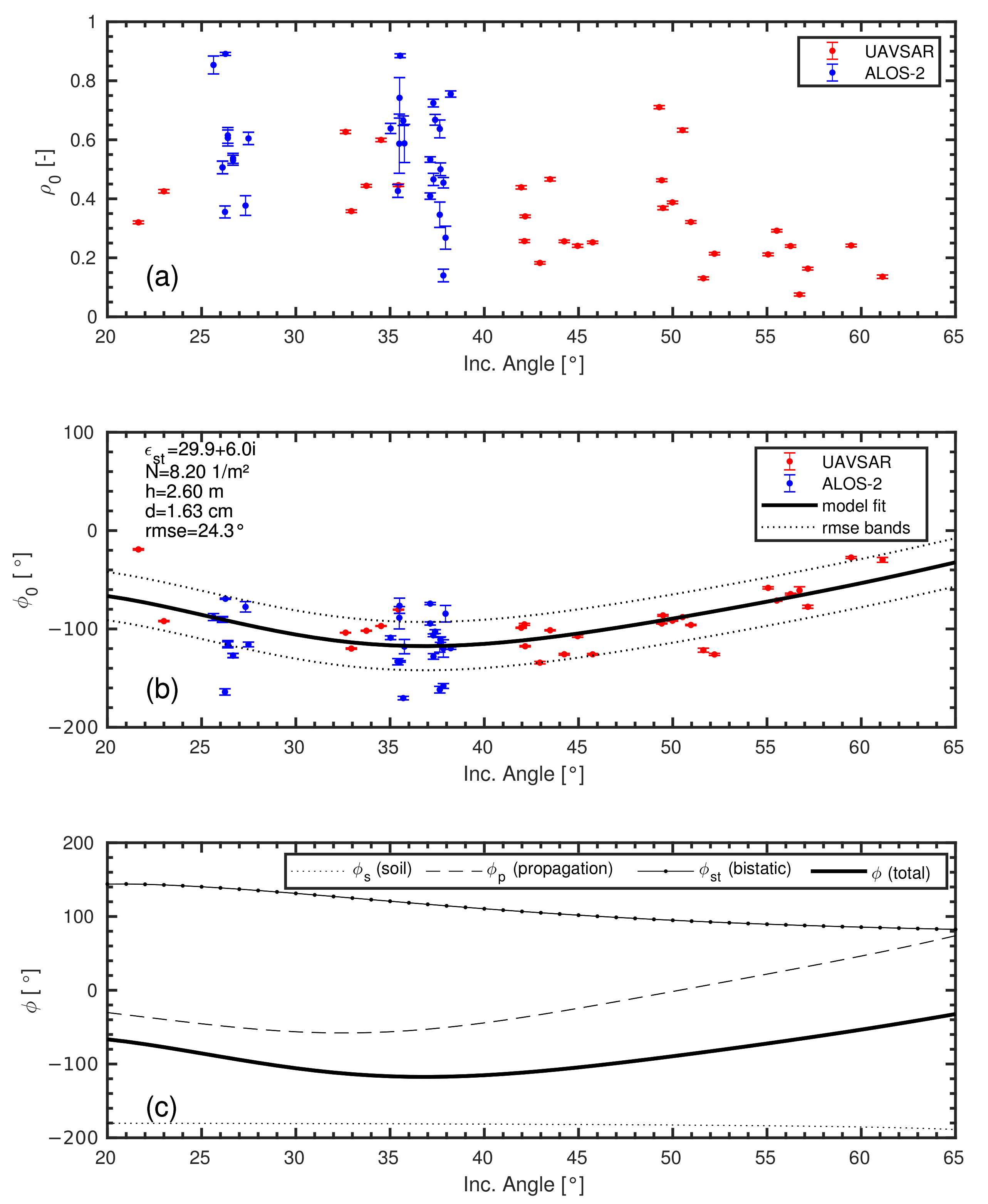
accounts for many scattering mechanisms and contributions. On a grown corn canopy, ϕ is modeled as a result of the sum of three single contributions
ϕ = ϕ p + ϕ s t + ϕ s ,
where ϕ p accounts for the phase term due to wave propagation through the canopy, ϕ s t for the forward scattering by the soil surface followed by bistatic scattering by the stalks, or the reverse process, and ϕ s for the specular reflection on the soil. Each one of these scattering mechanisms was evaluated following Ulaby’s model [17] and compared to SAR data.
Ulaby’s model [17] to be fitted accounts for the scattering interaction between the plant stalk and an underlying rough, moistened surface to compute (2). Corn plants were modeled as vertical dielectric cylinders, long enough relative to the wavelength to rely on the infinity cylinder scattering solution, which is given in the form of a series [27]
T H , V ( θ i , θ s ; k , a 0 , ε s t ) = n = + ( 1 ) n e i n θ s C n H , V ( θ i ; k , a 0 , ε s t ) ,
where T H , V is the normalized far-field scattering amplitude, the subscript states the polarization of the impinging wave onto a linear basis (H or V), θ i is the incidence angle relative to the plane containing the cylinder’s axis, and θ s is the azimuth scattered angle. The dependence of the functions C n H , V on the wavenumber k of the impinging wave, the radius a 0 and the complex dielectric constant ε s t of the cylinder is cumbersome and the reader is referred to [27] for their analytical expressions.
The solution given by (3) is applied two-fold. Firstly, Ulaby et al. [17] have shown that propagation in a layer comprising identical vertical cylinders randomly positioned on the ground may be modeled in terms of an equivalent dielectric medium characterized by a polarization-dependent complex index of refraction. The model assumed stalks are arranged with N cylinder per unit area and are far away enough such that multiple scattering is negligible. Hence, the phase constant of the index of refraction is used to compute the co-polarized phase difference for two-way propagation ( θ s = π in (3)). Secondly, the scattering solution in (3) is used to compute the phase difference between waves bistatically reflected by the stalks by considering specular scattering only ( θ s = 0 in (3)).
The first term on the right side in (2) computes the phase term due to the two-way, slanted propagation through the canopy,
ϕ p = 4 N h k tan θ Im { T H ( θ i , π ) } Im { T V ( θ i , π ) } ,
where h is stalk height. In (4), the scattering features of the stalks are accounted for in the T H , V amplitudes, where canopy bulk features are accounted for in the stalk density N and in h. The scattered angle is evaluated at the forward direction ( θ s = π ) [27].
The second term in (2) accounts for the phase term resulting from forward scattering by the soil surface followed by bistatic scattering by the stalks, or the reverse process,
ϕ s t = tan 1 Im { T H ( θ i , 0 ) / T V ( θ i , 0 ) } Re { T H ( θ i , 0 ) / T V ( θ i , 0 ) } ,
where the solution should be sought in the domain ( π , π ] . Here, θ s = 0 accounted for the specular direction.
The third term in (2) is the contribution from specular reflection on the soil through Fresnel reflection coefficients R H and R V [25]
ϕ s = tan 1 Im { R H ( θ i , ε s ) / R V ( θ i , ε s ) } Re { R H ( θ i , ε s ) / R V ( θ i , ε s ) } ,
where ε s is the complex dielectric constant of the soil surface underlying the canopy. The contribution of this term is about −180° due to the small imaginary part of ε s in typical soils and the difference in sign between R H and R V . Because of this term, total co-polarized phase difference ϕ , over grown corn canopies yields negative values on absolute calibrated polarimetric images.

2.2. Sensitivity Analysis of the Model Parameters

The three phase terms defined from (4) to (6) account respectively for the phase difference by propagation through the stalks, by the bistatic reflection, and by the soil. Each of these terms has different contributions to the total co-polarized phase difference in (2). In what follows, a sensitivity analysis will be carried out, where frequency will be fixed at an intermediate 1.25 GHz , that is, between those of UAVSAR and ALOS-2/PALSAR-2.
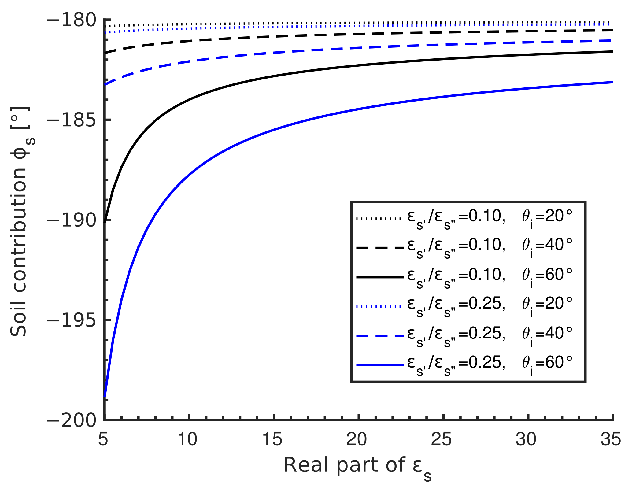
Among the three terms, the soil term ϕ s has a simple dependency on the soil’s complex dielectric constant ε s = ε s + i ε s . A typical imaginary-to-real ratio of ε s is 0.10, and commonly used empirical models predict this ratio to be as large as 0.25 [28,29,30]. Then, it follows from Figure 1 that the ϕ s dynamic range is less than 16° for an imaginary-to-real ratio of 0.10 (black lines) and 0.25 (blue lines). Three incidence angles 20°, 40°, and 60° are evaluated. Then, for a typical observation geometry at 40° incidence angle, the sensitivity to the dielectric constant shown by ϕ s is of little relevance to the total phase difference.
The propagation term in (4) has a linear dependence with the stalk density N and with the stalk height h. Moreover, since they are of the same order of magnitude, the effect of varying N or h on ϕ p will be equivalent. Conversely, the a 0 and ε s t are nonlinear model parameters through T H , V 
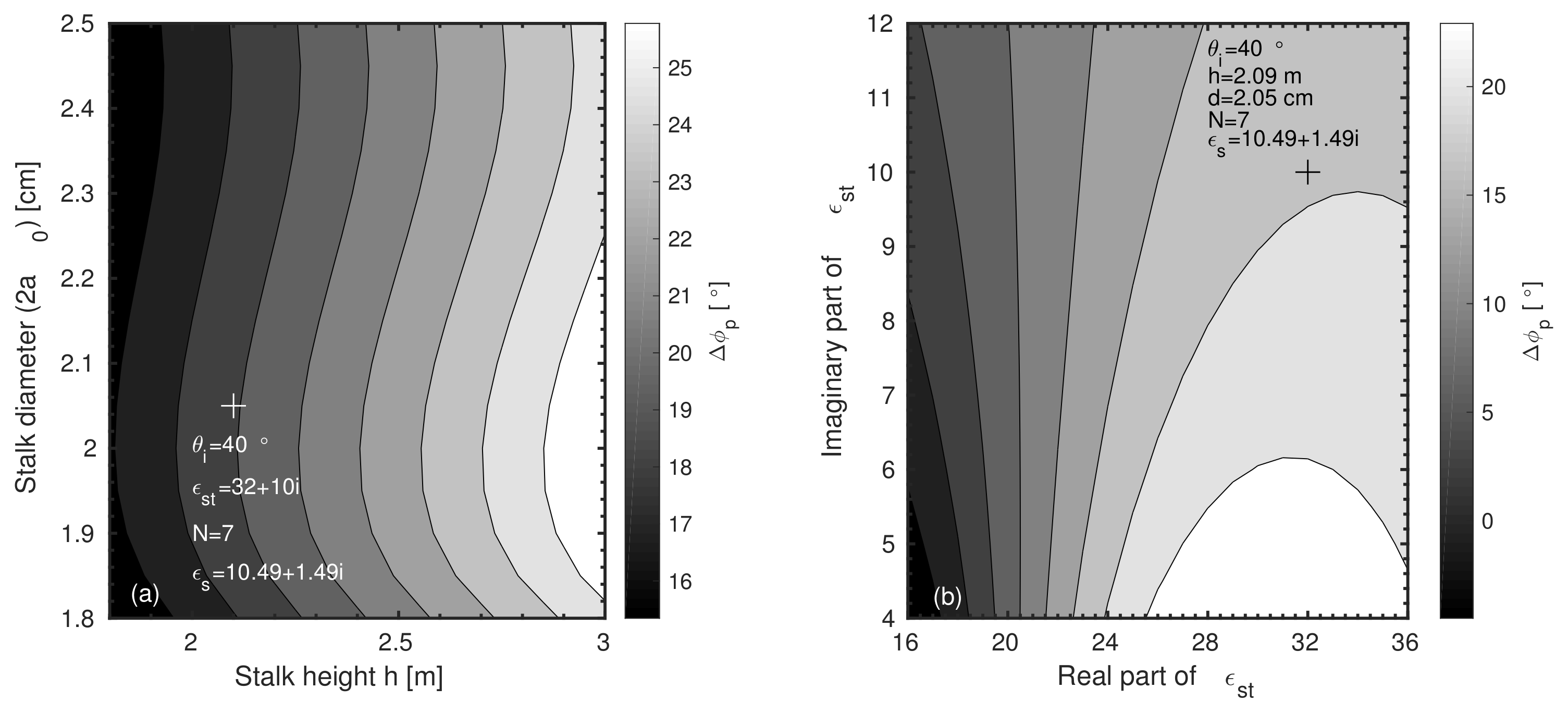
and the following sensitivity analysis will be focused on them. First, contour levels depicting the dependence of ϕ p on a 0 and h at θ i = 40 ° are shown in Figure 2a. The contours are variations of ϕ p computed as
Δ ϕ p = ϕ p a 0 Δ a 0 + ϕ p h Δ h ,
where it is understood that the other three terms involving derivatives (on ε s t , ε s t , and N) were computed and evaluated from the mean values collected on the ground, and these are indicated in the inset in Figure 2a.
A significant gradient indicated a high sensitivity to stalk height. This related to the linear term h in (4). Conversely, a small sensitivity on a 0 is related to a cancellation effect due to the difference operator in (4), since both T H and T V depend on a 0 . The model exhibits Δ ϕ p 20 ° when evaluated at the ground measurements (white ‘+’-mark in Figure 2a). For a better comparison to ground measurements, stalk diameter d = 2 a 0 instead of stalk radius a 0 is shown. Since N and h are of the same order, contours for ϕ p varying N instead of h will result in sensitivities similar, slightly smaller though, to the ones depicted in Figure 2a.
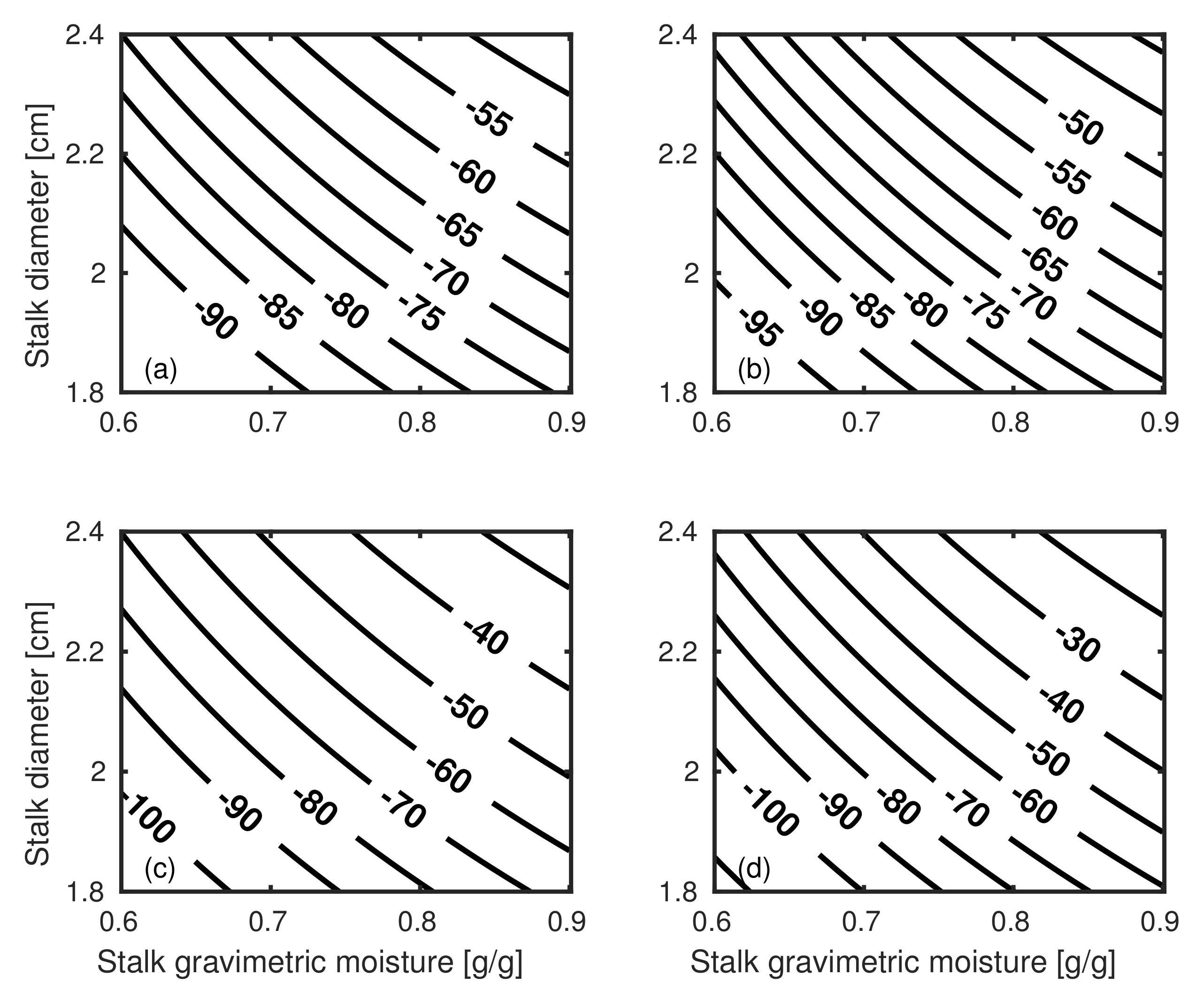
The sensitivity analysis on ϕ p for the real ε s t and imaginary ε s t parts of ε s t is shown in Figure 2b, where the inset indicates the parameters the model is evaluated at. Here, the contours range from around 0° to 20°, accounting for a larger sensitivity on ε s t in relation to that on h. However, Δ ϕ p 18 ° when evaluated at the ground measurements, similar to the sensitivity found in Figure 2a.
The bistatic term ϕ s t does not depend on h nor N. Moreover, overall the variation of ϕ s t on a 0 ranges from −7° to −2° with about −5° of variation with the model evaluated at the ground measurements. Hence, the contribution of the bistatic term to the overall model sensitivity is negligible. Similar results are reached for the sensitivity of ϕ s t on ε s t and ε s t .
The aforementioned analysis for Δ ϕ p and Δ ϕ s t considered a fixed incidence angle θ i = 40 ° . Computing the contour levels at different angles showed that:
  • At θ i = 20 ° , the ϕ p variations evaluated at the ground measurements are Δ ϕ p = 0 ° on the 2 a 0 , h -space and Δ ϕ p = 2 ° on ε s t , ε s t -space;
  • Similarly, at θ i = 60 ° resulted in Δ ϕ p = 26 ° and Δ ϕ p = 28 ° ;
  • At both θ i = 20 ° and θ i = 60 ° , Δ ϕ s t is bounded between −6° and −3°.
From these remarks, it turns out that sensitivity improved with increasing incidence angles for ϕ p , whereas the contribution to the overall sensitivity of the ϕ s t term is negligible.

2.3. Microwave Dielectric Constant of Stalk from Gravimetric Measurements

The propagation and bistatic terms in (4) and (5) depend on stalk diameter and dielectric constant through the far-field solution in (3). Whereas the collection of a 0 is straightforward from the ground, ε s t requires tuned laboratory measurement techniques [31]. From a large set of dedicated measurements, semi-empirical models relating bulk vegetation dielectric properties with vegetation moisture were developed by Ulaby and El Rayes [32], and Mätzer [26]. These are shown in Figure 3 for the vegetation moisture within the stalks. Concerning the range of validity, a slight drawback in Ulaby and El Rayes’ model is the upper bound of vegetation moisture used to fit the data. In effect, the model was fitted for gravimetric moisture m g in the range 0.0–0.7 g/g ([25], Chapter 4-9.2). On the other hand, Mätzer’s model [26] comprised measurements with larger moisture contents, which allowed setting an empirical fitting with m g in the range 0.5–0.9 g/g. Since typical gravimetric moisture for growth corn stalks is larger than 0.6 g/g, Mätzler’s model is better suited and will be used here to estimate the dielectric constant of vegetation material within corn stalks. Its input parameters are gravimetric moisture of plant stalks and frequency of the impinging wave. In Figure 3, note the trend in Ulaby and El Rayes’ model of larger dielectric values with respect to those in Mätzer’s model.

2.4. Study Area and Ground Data Collection

The dataset to fit the Ulaby’s incoherent multi-parameter model was taken from the Soil Moisture Active Passive Validation Experiment 2012 (SMAPVEx12) over southwest of Winnipeg, Manitoba, Canada, centered on the town of Elm Creek (98°0′23″ W, 49°40′48″ N) [11,33] and from intensive campaigns led by the SAOCOM mission’s science team near the town Monte Buey (32°55′11″ W, 62°27′22″ S), located in central Argentina over Pampas Plain. With these datasets, co-polarized phase measurements on grown corn fields covered incidence angles roughly from 20° to 60°.
In Canada, eight corn fields were imaged by UAVSAR at peak biomass on 17 July 2012. Each acquisition of the UAVSAR comprised four main flight lines with different incidence angles totaling 32 data points. Vegetation was characterized within a one-day window from the flight day: stalk height and diameter were measured. The former was measured with a meter tape and the latter with a caliper over 10 plants within the field selected at random positions. Then, the 10-plant average is computed. Stalk gravimetric moisture was also measured on a less frequent basis, though, due to time-consuming laboratory procedures. Five plants along two rows (ten in total) were collected, bagged appropriately, and then weighted before and after the samples were placed in drying facilities to quantify their water content [11]. A summary of the stalk features for the eight fields in Canada is shown in Table 1.
In Argentina, CONAE has the largest instrumented site over croplands dedicated to calibrating the soil moisture retrieval algorithm for the SAOCOM 1A and 1B mission. In March, April, and June 2017, intensive campaigns over a 140 × 100 km region were conducted and basic ground information over 20 corn fields among other crop types was gathered. Ground information included 0–5-cm soil moisture, stalk height, and till status. Stalk height measurements were taken at convenient positions while the plant was standing in the field. Measurements involving the removal of the plant were disregarded due to time-constraints. The stalk height is summarized in Table 1. These fields were imaged by ALOS-2/PALSAR-2 on several dates totaling 30 data points.

2.5. SAR Data and Its Quality and Processing Chain

Airborne UAVSAR provided full-polarimetric imagery over Canada with local incidence angles ranging from 20° to 60°. It measured complex scattering coefficients at a frequency of 1.258 GHz. Co-polarized phase measurements are given with a root mean squared phase error ∼ 5.3 ° and always smaller than 10 ° [34]. The pixel size on the ground projected image is 5.0 × 7.2 m onto a swath of 20 km .
As read from its metadata, UAVSAR imagery has the coherence matrix as a native image format where S H H S V V * is readily extracted from. Multi-looked (12 pixels in azimuth by 3 pixels in range) and ground range projected data were used. The ground projection method was nearest neighbor. With the S H H S V V * -images, local incidence angle bands were also provided.
Concurrent with the ground measurements over Argentina, fully polarimetric images were acquired by satellite-borne ALOS-2/PALSAR-2 sensor at 1.236 GHz in High-sensitive Full Polarimetry mode with a 50-km swath width at two incidence angle ranges: 25–30° and 30–35°. This sensor delivered co-polarized phase difference measurements with an imbalance better than 0.618 ° ([35], Table 3).
For ALOS-2/PALSAR-2, the processing chain started with radiometric calibration from Single Look Complex (SLC) scenes. Subsequently, multilooking was applied (4 pixels in azimuth by 2 pixels in range) to obtain an approximate square pixel and improve the images’ radiometric quality. Coherence matrices were computed and then geocoded to a 12 × 12 m ground pixel size using bilinear resampling. As the final product, output bands for complex scattering product S H H S V V * and for local incidence angle were generated.

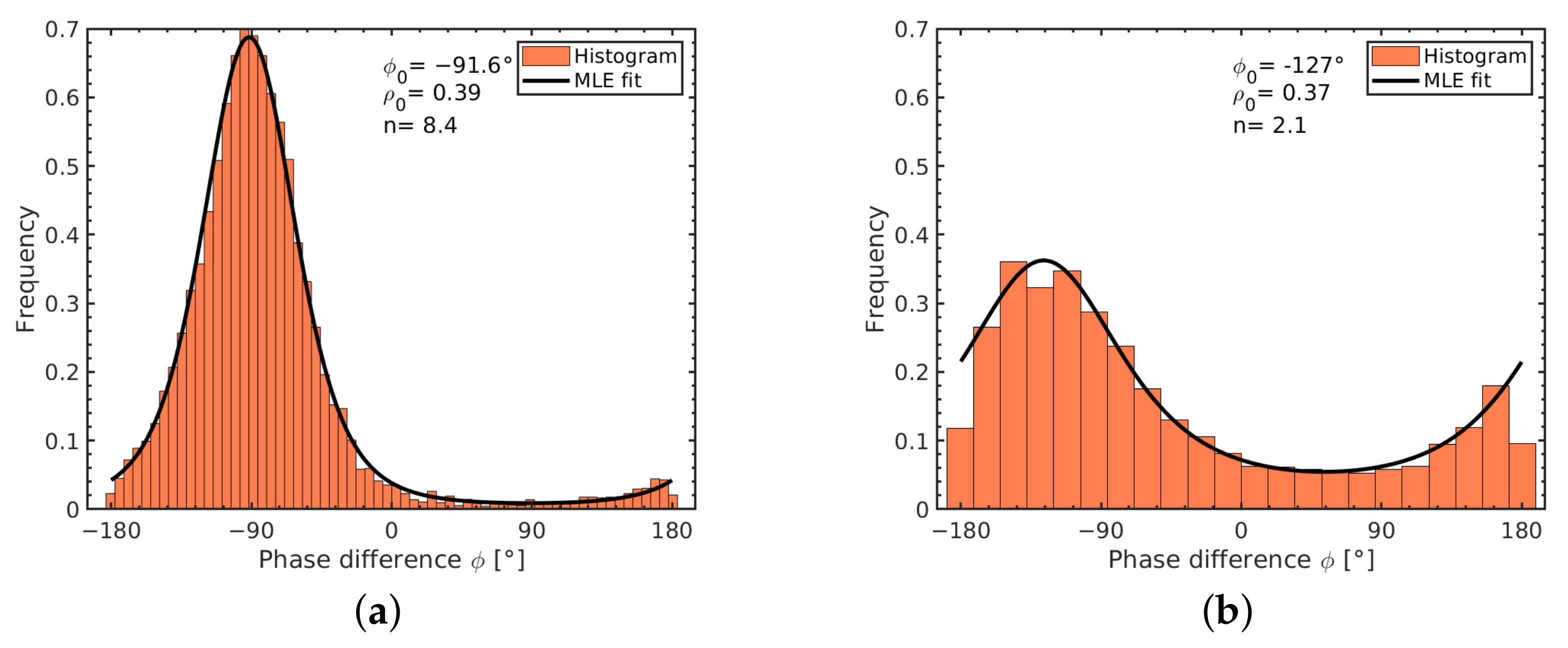
2.6. Polarimetric Observable ϕ

With the above-mentioned phase-calibrated images, the derivation of the absolute co-polarized phase difference defined in (1) is given by
ϕ = a r g ( S H H S V V * ) ,
where S H H and S V V are the co-polarized complex scattering amplitudes, and * denotes a complex conjugate. In (8), ϕ is defined in the range π < ϕ π . The statistical distribution of ϕ for a speckled image is known, and its closed-form expression is [36]
P ϕ ( n ) ( ϕ ; ρ 0 , ϕ 0 ) = Γ ( n + 1 / 2 ) ( 1 ρ 0 2 ) n β 2 π Γ ( n ) ( 1 β 2 ) + + ( 1 ρ 0 2 ) n 2 π 2 F 1 n , 1 ; 1 / 2 ; β 2
with β = ρ 0 cos ( ϕ ϕ 0 ) where 2 F 1 n , 1 ; 1 / 2 ; β 2 is a Gauss hypergeometric function. In (9), ρ 0 is the correlation between S H H and S V V * , also known as coherence, ϕ 0 is the phase difference of the sample, Γ ( · ) is the gamma function, and n is the equivalent number of looks, which is estimated by means of a matrix-variate estimator based on the trace of the product of the covariance matrix C with itself ( tr ( C C ) ), thus using all polarimetric information [37].

3. Results

3.1. Co-Polarized Phase Difference ϕ 0 Estimation

The parameters ϕ 0 and ρ 0 in (9) were estimated using a Maximum Likelihood Estimation (MLE) [38], where (9) is the likelihood function to be maximized constrained to the observed SAR data. The MLE technique applied to multilooked histograms led to the fittings shown in Figure 4. Here, Figure 4a,b display the histogram for a 2.27 m-height corn field imaged with UAVSAR, and a 2.00 m-height corn field imaged with ALOS-2/PALSAR-2, respectively. The number of looks n estimated from the above matrix-variate estimator is also shown. Thus, the co-polarized phase difference estimator ϕ 0 is computed for each sampling site on each acquisition day. Furthermore, uncertainties in the estimates are computed with a 95% confidence level.

3.2. Ulaby’s Model Fitting to SAR Data

With the model described in Section 2.1 and the HH-VV phase estimation methodology explained in Section 3.1, a nonlinear least-squares fitting of the measurements against the model is performed, as shown in Figure 5. The upper panel shows the estimated coherence ρ 0 and its uncertainties as bars resulting from the MLE technique. The middle panel shows the fitting itself with the thick black as the best-fitted total co-polarized phase difference ϕ 0 . The dotted bands represent the interval defined by the root mean squared error (rmse). Fitted model parameters are also shown. Each term ϕ p , ϕ s t , and ϕ s is depicted separately in Figure 5c.
Overall, a good agreement is shown in the view of the dispersion found in the ground measurements, most remarkably in stalk height (see Table 1). A slight overestimation is expected since the corn plant developed above the stalk, resulting in an overall plant structure taller than the stalk itself. Furthermore, the vegetation material within the stalks occupied a smaller volume within the stalk rind, thus leading to an underestimation in the fitted diameter since the outer layer comprising the rind is almost dry. By means of Mätzler’s vegetation model, shown in Figure 3, the fitted real part ε s t = 29.9 corresponds to a m g = 0.78   g / g , close to the laboratory-measured m g = ( 0.82 ± 0.01 )   g / g . Moreover, the ϕ 0 estimates with lower ρ 0 (corresponding to 50° and 65° in Figure 5b) fitted well, indicating that using an MLE technique over the whole histogram resulted in sound, reliable estimates.
With regards to the dependency on the incidence angle shown in Figure 5c, the propagation term becomes relevant for large θ i due to increasing interaction with dielectric stalks for slanted propagation paths through the corn plants. The soil term sets a reference level almost insensitive to incidence angle variations.
The Canada campaign collected corn parameters regularly, covering most of the development of the corn plants. For further assessment, the same procedure described above was applied to the corresponding UAVSAR dataset on dates before peak biomass on 17 July 2012. Table 2 summarizes the fitted model parameters and the root mean squared error on 5, 8, 14, and 17 July 2012. The corresponding ground measurements are grouped by dates to compensate for missing data, thus covering all eight sites.
While the trend in stalk height seemed to correspond to the plant’s growth, the fitted ϕ 0 is somewhat insensitive to stalk diameter, likely due to the sensitivity of the underlying model to these parameters and the dispersion in model parameters. Again, an underestimation of the diameter is expected due to the smaller volume of the vegetation material within the stalks.
On the other hand, the stalk dielectric constant showed a significant sensitivity. With the measured stalk gravimetric moisture shown in Table 2, a straightforward comparison of fitted ε s t with m g is made with the aid of Mätzler’s model shown in Figure 3. In effect, as followed from Figure 3, the range 0.834–0.847 g/g corresponded to the ε s t range 32–34, which is in reasonable agreement with the corresponding fitted parameter. Similarly, the range 0.811–0.834 g/g corresponded to ε s t in the range 31–32. The complex dielectric part is governed by the salinity of the vegetation bulk material. Hence, it can be regarded as a second-order effect in relation to the real part dielectric constant and, therefore, its low sensitivity.
Finally, as mentioned in the introduction, some techniques make the estimation of crop height available. Hence, stalk height might be regarded as a known parameter in specific applications. On the other hand, stalk diameter and gravimetric moisture are plant features that involve time-consuming gathering procedures. If copolarized phase measurements are available over a known corn field at some late stage, Figure 6 can aid in parameter retrieval provided some guess in stalk gravimetric moisture or diameter is at hand. Usually, relationships between diameter and height are available for corn and maize elsewhere (e.g., [39]). The contour levels in Figure 6 were evaluated for several stalk heights by parameterizing the stalk dielectric constant ε s t with gravimetric moisture m g using Mätzler’s model.

4. Discussion

Availability of a fully polarimetric dataset involving airborne and satellite-borne images and stalk dielectric, structural, and spatial parameters enabled a multi-parameter modeling over corn fields. The model considered here for the co-polarized phase difference comprised three incoherent contributions with different sensitivities. Whereas the soil term set an almost constant reference level of around -180°, propagation and bistatic terms had a marked dependency with height, diameter, and moisture of the stalks. By adding them up, the incoherent, interaction-based model fitting showed good agreement with UAVSAR and ALOS-2/PALSAR-2 acquisitions, provided the dispersion in the ground measurements be accounted for. By separating each of the contributions, a more accurate understanding of crop interaction is made, advancing previous research where a full explanation of observation data could not be given since considerable modeling efforts were required [20,24]. Moreover, a number of dedicated radar experiments [15,16,40] with detailed field measurements collected on corn fields can benefit from incorporating a co-polarized phase model to extend their findings to phase-related observables, since modeling efforts associated with these experiments were limited to intensity-related observables only.
More accurate crop scattering models will likely include detailed canopy physical attributes, other than only stalk height and width, such as leaf area index, leaf orientation distribution, and leaf size [41], among others. As a result, a direct relationship of the scattering with plant biophysical parameters might not be easy to develop. On the other hand, scattering models with interaction at higher orders for randomly distributed vertical cylinders rely on Monte Carlo simulations or iterative methods [18]. Thus, the few parameters implied in the Ulaby’s model and its straightforward analytical expression highlight its usefulness.
From the sensitivity analysis on Ulaby’s model described in Section 2.2, the stalk height resulted in the highest sensitivity on the propagation term ϕ p for all the incidence angles. This goes in line with the application mentioned at the end of Section 3, where the contours shown in Figure 6 leverage the stalk height retrieval from other remotely-sensed techniques (i.e., [21]) through the improved sensitivity of the term ϕ p in the total ϕ 0 . In this regard, corn height estimates with a root mean square error around 40–50 cm over a growing season were demonstrated with machine learning techniques over a dataset of polarimetric SAR observables at the C-band [21]. This study also highlighted the relevance of polarimetric features related to double-bounce scattering (i.e., ϕ s t ) [21]. Moreover, model parameterization by stalk gravimetric moisture content instead of its complex dielectric constant using Mätzler’s model demonstrated a potential resource for dimensionality reduction, thus helping future application-oriented developments.
Several techniques are usually validated with data from airborne campaigns and then expected to be readily applied with similar levels of accuracy to imagery acquired by orbiting sensors. In the case analyzed in this research, field-based estimates from satellite-borne acquisitions such as those of ALOS-2/PALSAR-2 were clearly constrained by histograms with fewer data points since the larger pixel sizes involved were compared to airborne acquisitions. With the sound histogram-based, matrix-variate Maximum Likelihood Estimation technique described in Section 3.1, the estimates from ALOS-2/PALSAR-2 resulted in slightly larger, otherwise reasonably bounded, uncertainties than UAVSAR ones.
With the increasing availability of L-band space-borne SAR missions adding to existing C-band SAR resources (e.g., European Space Agency’s Sentinel-1), multi-frequency methodologies may become fully operational in the near future. The multi-frequency approach exploits different penetration capabilities into the vegetation canopy. For instance, these enhanced capabilities can potentially circumvent typical issues regarding the classification of crops with similar architectures such as corn and sorghum, the latter widely spread in America and Africa. To a greater extent, if multi-frequency polarimetric SAR data become available, polarimetric modeling such as the Ulaby–Mätzler model can enhance further corn plant parameter retrieval.

5. Conclusions

Research on crop scattering processes can primarily benefit from fully polarimetric data. In addition to usual power scattering coefficients, a promising polarimetric observable for crop monitoring is the phase difference between the co-polarized complex scattering amplitudes. By leveraging the penetration capabilities at the L-band, fully polarimetric SAR missions become worthwhile over croplands. This study presents a scattering model coupled with a semi-empirical dielectric model for co-polarized phase differences resulting from the interaction of microwaves with grown corn canopies. The dataset included airborne and space-borne fully polarimetric SAR data with incidence angles ranging from 20° to 60°. A set of 60 data points was analyzed and used to perform an experimental data fitting with a nonlinear least-squares technique. The results showed a satisfactory agreement for corn co-polarized phase differences at the field scale, with an RMSE of around 24.3° considering airborne and space-borne acquisitions. Compared with available studies on corn phase differences with SAR data, this research provides a new perspective on using phase-related observables on fully polarimetric SAR data over corn fields.

Author Contributions

Conceptualization, M.E.B. and C.L.-M.; formal analysis, M.E.B.; funding acquisition, C.L.-M.; investigation, M.E.B.; methodology, M.E.B.; resources, M.E.B.; software, D.S.R.; validation, M.E.B. and D.S.R.; visualization, M.E.B.; writing—original draft, M.E.B. and D.S.R.; writing—review and editing, C.L.-M. All authors have read and agreed to the published version of the manuscript.

Funding

This research was partially funded by the Argentinean National Scientific and Technical Research Council (CONICET, project PICT 2015 N° 3689), by the Spanish Ministry of Science and Innovation (project CICYT RTI2018-099008-B-C21/AEI/10.13039/501100011033 “Sensing with pioneering opportunistic techniques”) and by the grant to “CommSensLab-UPC” Excellence Research Unit Maria de Maeztu (MINECO grant).

Institutional Review Board Statement

Not applicable.

Informed Consent Statement

Not applicable.

Data Availability Statement

The data are not publicly available due to license restrictions.

Acknowledgments

Special thanks to Heather McNairn and CONAE for sharing part of the Canada and Argentina ground data, respectively. The authors acknowledged Avik Bhattacharya for revising the manuscript and for his valuable comments.

Conflicts of Interest

The authors declare no conflict of interest.

References

  1. McNairn, H.; Brisco, B. The application of C-band polarimetric SAR for agriculture: A review. Can. J. Remote Sens. 2004, 30, 525–542. [Google Scholar] [CrossRef]
  2. Li, H.; Zhang, C.; Zhang, S.; Atkinson, P.M. Crop classification from full-year fully-polarimetric L-band UAVSAR time-series using the Random Forest algorithm. Int. J. Appl. Earth Obs. Geoinf. 2020, 87, 102032. [Google Scholar] [CrossRef]
  3. Larrañaga, A.; Álvarez Mozos, J. On the Added Value of Quad-Pol Data in a Multi-Temporal Crop Classification Framework Based on RADARSAT-2 Imagery. Remote Sens. 2016, 8, 335. [Google Scholar] [CrossRef] [Green Version]
  4. Erten, E.; Lopez-Sanchez, J.M.; Yuzugullu, O.; Hajnsek, I. Retrieval of agricultural crop height from space: A comparison of SAR techniques. Remote Sens. Environ. 2016, 187, 130–144. [Google Scholar] [CrossRef] [Green Version]
  5. Lopez-Sanchez, J.M.; Vicente-Guijalba, F.; Erten, E.; Campos-Taberner, M.; Garcia-Haro, F.J. Retrieval of vegetation height in rice fields using polarimetric SAR interferometry with TanDEM-X data. Remote Sens. Environ. 2017, 192, 30–44. [Google Scholar] [CrossRef] [Green Version]
  6. Ndikumana, E.; Ho Tong Minh, D.; Dang Nguyen, H.T.; Baghdadi, N.; Courault, D.; Hossard, L.; El Moussawi, I. Estimation of Rice Height and Biomass Using Multitemporal SAR Sentinel-1 for Camargue, Southern France. Remote Sens. 2018, 10, 1394. [Google Scholar] [CrossRef] [Green Version]
  7. Barber, M.; Bruscantini, C.; Grings, F.; Karszenbaum, H. Bayesian Combined Active/Passive (B-CAP) Soil Moisture Retrieval Algorithm. IEEE J. Sel. Top. Appl. Earth Obs. Remote Sens. 2016, 9, 5449–5460. [Google Scholar] [CrossRef]
  8. Das, N.N.; Entekhabi, D.; Dunbar, R.S.; Colliander, A.; Chen, F.; Crow, W.; Jackson, T.J.; Berg, A.; Bosch, D.D.; Caldwell, T.; et al. The SMAP mission combined active-passive soil moisture product at 9 km and 3 km spatial resolutions. Remote Sens. Environ. 2018, 211, 204–217. [Google Scholar] [CrossRef]
  9. Hensley, S.; Michel, T.; Van Zyl, J.; Muellerschoen, R.; Chapman, B.; Oveisgharan, S.; Haddad, Z.S.; Jackson, T.; Mladenova, I. Effect of Soil Moisture on polarimetric-interferometric repeat pass observations by UAVSAR during 2010 Canadian Soil Moisture campaign. In Proceedings of the 2011 IEEE International Geoscience and Remote Sensing Symposium, Brussels, Belgium, 11–16 July 2011; pp. 1063–1066. [Google Scholar] [CrossRef]
  10. Morandeira, N.S.; Franco, M.; Barber, M.; Grings, F. Modeling Bare Soil L-Band Polarimetric H-α Values Using a Second-Order SPM Model. IEEE Geosci. Remote Sens. Lett. 2016, 13, 399–403. [Google Scholar] [CrossRef]
  11. McNairn, H.; Jackson, T.J.; Wiseman, G.; Bélair, S.; Berg, A.; Bullock, P.; Colliander, A.; Cosh, M.H.; Kim, S.B.; Magagi, R.; et al. The Soil Moisture Active Passive Validation Experiment 2012 (SMAPVEX12): Prelaunch Calibration and Validation of the SMAP Soil Moisture Algorithms. IEEE Trans. Geosci. Remote Sens. 2015, 53, 2784–2801. [Google Scholar] [CrossRef]
  12. NASA Jet Propulsion Laboratory. NASA-ISRO SAR (NISAR) Mission Science Users’ Handbook; NASA Jet Propulsion Laboratory: Pasadena, CA, USA, 2018; p. 261. [Google Scholar]
  13. ESA. Copernicus L-Band SAR Mission Requirements Document. Available online: https://esamultimedia.esa.int/docs/EarthObservation/Copernicus_L-band_SAR_mission_ROSE-L_MRD_v2.0_issued.pdf (accessed on 8 November 2021).
  14. FAOSTAT: The Food and Agriculture Organization (FAO) Statistics. Available online: http://www.fao.org/faostat/en/#data/QC (accessed on 25 February 2021).
  15. Joseph, A.T.; van der Velde, R.; O’Neill, P.E.; Lang, R.H.; Gish, T. Soil Moisture Retrieval During a Corn Growth Cycle Using L-Band (1.6 GHz) Radar Observations. IEEE Trans. Geosci. Remote Sens. 2008, 46, 2365–2374. [Google Scholar] [CrossRef] [Green Version]
  16. Sharma, A.; Lang, R.H.; Kurum, M.; O’neill, P.E.; Cosh, M.H. L-Band Radar Experiment and Modeling of a Corn Canopy Over a Full Growing Season. IEEE Trans. Geosci. Remote Sens. 2020, 58, 5821–5835. [Google Scholar] [CrossRef]
  17. Ulaby, F.T.; Held, D.; Dobson, M.C.; McDonald, K.C.; Senior, T.B.A. Relating Polarization Phase Difference of SAR Signals to Scene Properties. IEEE Trans. Geosci. Remote. Sens. 1987, GE-25, 83–92. [Google Scholar] [CrossRef]
  18. Sarabandi, K.; Polatin, P.F.; Ulaby, F.T. Monte Carlo simulation of scattering from a layer of vertical cylinders. IEEE Trans. Antennas Propag. 1993, 41, 465–475. [Google Scholar] [CrossRef]
  19. Karam, M.A.; Fung, A.K. Electromagnetic scattering from a layer of finite length, randomly oriented, dielectric, circular cylinders over a rough interface with application to vegetation. Int. J. Remote Sens. 1988, 9, 1109–1134. [Google Scholar] [CrossRef]
  20. Skriver, H.; Svendsen, M.T.; Thomsen, A.G. Multitemporal C- and L-band polarimetric signatures of crops. IEEE Trans. Geosci. Remote Sens. 1999, 37, 2413–2429. [Google Scholar] [CrossRef]
  21. Xie, Q.; Wang, J.; Lopez-Sanchez, J.M.; Peng, X.; Liao, C.; Shang, J.; Zhu, J.; Fu, H.; Ballester-Berman, J.D. Crop Height Estimation of Corn from Multi-Year RADARSAT-2 Polarimetric Observables Using Machine Learning. Remote Sens. 2021, 13, 392. [Google Scholar] [CrossRef]
  22. Cable, J.W.; Kovacs, J.M.; Jiao, X.; Shang, J. Agricultural Monitoring in Northeastern Ontario, Canada, Using Multi-Temporal Polarimetric RADARSAT-2 Data. Remote Sens. 2014, 6, 2343–2371. [Google Scholar] [CrossRef] [Green Version]
  23. Lopez-Sanchez, J.M.; Ballester-Berman, J.D.; Hajnsek, I. First Results of Rice Monitoring Practices in Spain by Means of Time Series of TerraSAR-X Dual-Pol Images. IEEE J. Sel. Top. Appl. Earth Obs. Remote Sens. 2011, 4, 412–422. [Google Scholar] [CrossRef]
  24. Balenzano, A.; Mattia, F.; Satalino, G.; Davidson, M. Dense Temporal Series of C- and L-band SAR Data for Soil Moisture Retrieval Over Agricultural Crops. Sel. Top. Appl. Earth Obs. Remote Sens. IEEE J. 2011, 4, 439–450. [Google Scholar] [CrossRef]
  25. Ulaby, F.T.; Long, D.; Blackwell, W.; Elachi, C.; Fung, A.; Ruf, C.; Sarabandi, K.; van Zyl, J.; Zebker, H. Microwave Radar and Radiometric Remote Sensing; The University of Michigan Press: Ann Arbor, MI, USA, 2014. [Google Scholar]
  26. Mätzler, C. Microwave (1–100 GHz) dielectric model of leaves. IEEE Trans. Geosci. Remote Sens. 1994, 32, 947–949. [Google Scholar] [CrossRef]
  27. Ruck, G. Radar Cross Section Handbook; Number v. 2 in Radar Cross Section Handbook; Plenum Press: New York, NY, USA, 1970. [Google Scholar]
  28. Hallikainen, M.; Ulaby, F.; Dobson, M.; El-Rayes, M.; Wu, L.K. Microwave Dielectric Behavior of Wet Soil-Part I: Empirical Models and Experimental Observations. IEEE Trans. Geosci. Remote Sens. 1985, GE-23, 25–34. [Google Scholar] [CrossRef]
  29. Peplinski, N.R.; Ulaby, F.T.; Dobson, M.C. Dielectric properties of soils in the 0.3–1.3-GHz range. IEEE Trans. Geosci. Remote Sens. 1995, 33, 803–807. [Google Scholar] [CrossRef]
  30. Mironov, V.L.; Dobson, M.C.; Kaupp, V.H.; Komarov, S.A.; Kleshchenko, V.N. Generalized refractive mixing dielectric model for moist soils. IEEE Trans. Geosci. Remote Sens. 2004, 42, 773–785. [Google Scholar] [CrossRef]
  31. El-Rayes, M.A.; Ulaby, F.T. Microwave Dielectric Spectrum of Vegetation—Part I: Experimental Observations. IEEE Trans. Geosci. Remote Sens. 1987, GE-25, 541–549. [Google Scholar] [CrossRef]
  32. Ulaby, F.T.; El-Rayes, M.A. Microwave Dielectric Spectrum of Vegetation—Part II: Dual-Dispersion Model. IEEE Trans. Geosci. Remote Sens. 1987, GE-25, 550–557. [Google Scholar] [CrossRef]
  33. SMAP Validation Experiment 2012, Experimental Plan. Available online: https://smapvex12.espaceweb.usherbrooke.ca (accessed on 22 September 2021).
  34. Fore, A.; Chapman, B.; Hawkins, B.; Hensley, S.; Jones, C.; Michel, T.; Muellerschoen, R. UAVSAR Polarimetric Calibration. Geosci. Remote Sens. IEEE Trans. 2015, 53, 3481–3491. [Google Scholar] [CrossRef]
  35. Motohka, T.; Isoguchi, O.; Sakashita, M.; Shimada, M. Results of ALOS-2 PALSAR-2 Calibration and Validation After 3 Years of Operation. In Proceedings of the IGARSS 2018—2018 IEEE International Geoscience and Remote Sensing Symposium, Valencia, Spain, 22–27 July 2018; pp. 4169–4170. [Google Scholar]
  36. Lee, J.S.; Pottier, E. Polarimetric Radar Imaging: From Basics to Applications; CRC Press: Boca Raton, FL, USA, 2009. [Google Scholar] [CrossRef]
  37. Anfinsen, S.; Doulgeris, A.; Eltoft, T. Estimation of the Equivalent Number of Looks in Polarimetric Synthetic Aperture Radar Imagery. Geosci. Remote Sens. IEEE Trans. 2009, 47, 3795–3809. [Google Scholar] [CrossRef]
  38. Wasserman, L. All of Statistics: A Concise Course in Statistical Inference; Springer Texts in Statistics; Springer: New York, NY, USA, 2004. [Google Scholar]
  39. Umburanas, R.C.; Kawakami, J.; Eschemback, V.; Ribeiro Oliari, I.C. Effect of green manure and sources of phosphorus on the morphology and yield of maize plants. Braz. J. Appl. Technol. Agric. Sci. 2013, 6, 49–56. [Google Scholar] [CrossRef]
  40. Monsivais-Huertero, A.; Liu, P.W.; Judge, J. Phenology-Based Backscattering Model for Corn at L-Band. IEEE Trans. Geosci. Remote Sens. 2018, 56, 4989–5005. [Google Scholar] [CrossRef]
  41. Bracaglia, M.; Ferrazzoli, P.; Guerriero, L. A fully polarimetric multiple scattering model for crops. Remote Sens. Environ. 1995, 54, 170–179. [Google Scholar] [CrossRef]
Figure 1. Sensitivity of soil term on the real part of the dielectric constant. The imaginary part is assumed to be 0.10 (black lines) and 0.25 (blue lines) of the real part.
Remotesensing 13 04593 g001
Figure 2. Sensitivity analysis of model parameters. (a) Sensitivity of the propagation term on stalk height and diameter 2 a 0 . The ‘+’-mark indicates the average values for the dataset. (b) Sensitivity of propagation term on real ε s t and imaginary ε s t parts of ε s t .
Remotesensing 13 04593 g002
Figure 3. Microwave dielectric model for bulk vegetation from Ulaby and El Rayes [25,32] and from Mätzler [26].
Remotesensing 13 04593 g003
Figure 4. MLE fitting for speckled co-polarized phase difference histograms. (a) A 2.27-m-height corn field imaged by UAVSAR at incidence angle 49.98°. (b) A 2.00-m-eight corn field imaged by ALOS-2/PALSAR-2 at incidence angle 26.67°.
Remotesensing 13 04593 g004
Figure 5. Model fitting by nonlinear least-squares and estimated parameters. (a) Coherence ρ 0 . (b) Co-polarized phase difference ϕ 0 and model fitting. The fitted parameters are indicated. (c) Each contribution to the total phase difference is shown separately.
Remotesensing 13 04593 g005
Figure 6. ϕ -contours resulting from the evaluation of (2) when coupling Mätzler’s model with Ulaby’s. Frequency is fixed at 1.25 GHz and incidence angle is 40°. Model parameters now include m g instead of ε s t . Stalk height h is indicated. (a) h = 1.80   m . (b) h = 2.00   m . (c) h = 2.40   m . (d) h = 2.80   m . Contours are in degrees.
Remotesensing 13 04593 g006
Table 1. Corn stalk features from the ground data collection for two field campaigns in Canada and Argentina.
FeatureCanadaArgentina
(SMAPVex12)(CONAE)
# Fields [-]820
# Data points [-]3230
Stalk height h range [m]1.93–2.531.80–3.00
Stalk diameter d range [cm]1.85–2.35-
Stalk moisture m g range [g/g]0.811–0.834-
Stalk density N [1/ m 2 ]7.0–8.2-
Table 2. Stalk features as compared to the fitting and to the ground data from dates prior to peak biomass. Field campaign in Canada with UAVSAR. The di2electric constant on ground data is estimated from stalk moisture by means of Mätzler’s model shown in Figure 3.
Date
5 July 20128 July 201214 July 201217 July 2012
Fitted pars.
Height h [m]1.421.832.562.60
Diameter d [cm]1.801.801.801.80
Dielectric constant ε s t [-]30.6 + 6.0i31.4 + 6.0i32.0 + 6.0i24.9 + 6.0i
Density N [1/m2]7.157.398.168.20
Root mean sq. error [°]16.320.821.822.3
Ground data
Height h range [m]1.19–1.771.93–2.53
Diameter d range [cm]2.00–2.291.85–2.35
Moisture m g range [g/g]0.834–0.8470.811–0.834
Dielectric constant (real part) ε s t [-]32–3431–32
Publisher’s Note: MDPI stays neutral with regard to jurisdictional claims in published maps and institutional affiliations.

