Spectral and Spatial Feature Integrated Ensemble Learning Method for Grading Urban River Network Water Quality

Abstract

Urban river networks have the characteristics of medium and micro scales, complex water quality, rapid change, and time–space incoherence. Aiming to monitor the water quality accurately, it is necessary to extract suitable features and establish a universal inversion model for key water quality parameters. In this paper, we describe a spectral- and spatial-feature-integrated ensemble learning method for urban river network water quality grading. We proposed an in situ sampling method for urban river networks. Factor and correlation analyses were applied to extract the spectral features. Moreover, we analyzed the maximum allowed bandwidth for feature bands. We demonstrated that spatial features can improve the accuracy of water quality grading using kernel canonical correlation analysis (KCCA). Based on the spectral and spatial features, an ensemble learning model was established for total phosphorus (TP) and ammonia nitrogen (NH₃-N). Both models were evaluated by means of fivefold validation. Furthermore, we proposed an unmanned aerial vehicle (UAV)-borne water quality multispectral remote sensing application process for urban river networks. Based on the process, we tested the model in practice. The experiment confirmed that our model can improve the grading accuracy by 30% compared to other machine learning models that use only spectral features. Our research can extend the application field of water quality remote sensing to complex urban river networks.

1. Introduction

Among rivers, small- and medium-sized rivers are often ignored in daily water quality monitoring. However, these rivers are places where water pollution often occurs [1], especially in the cities of developing countries [2,3]. The most common pollutants are nitrogen (N) and phosphorus (P), which may lead to algal blooms [4,5,6]. In addition, for a single river, water quality is usually different in different watersheds and it constantly changes over time. Therefore, a comprehensive, fine-scale and high-frequency monitoring method is needed to improve urban river water quality monitoring programs.

Remote sensing technology can rapidly monitor a large area. Recently, there have been a large number of studies on remote sensing water quality monitoring [7]. The purpose of remote sensing water quality inversion is to establish an accurate relationship between image features and water quality. A large quantity of these studies focused on Case 1 waters and Case 2 waters, such as seas, large rivers, and lakes [8,9,10]. Moreover, these studies were mainly based on images of specific bands [11]. However, the water quality and optical properties of different urban rivers may vary greatly [12]. Thus, considering the complexity of urban water systems, it is necessary to extract suitable features and establish a universal inversion model for key water quality parameters.

Spectral features are the most important features in water quality remote sensing. Different constituents in water have different optical properties. Spectral feature analysis aims to extract the key bands that have a high correlation with the water quality parameters. Dimensionality reduction [13], clustering [14], and ranking [15] are the most commonly used methods for extracting the feature bands. In addition, regarding the water quality parameters, the correlation between the spectral features and water quality parameters also needs to be analyzed [16]. Bandwidth is another important spectral feature that needs to be determined for water quality inversion and sensor production [17]. The sensitive bands of water quality parameters have specific wavelength ranges. The information from other bands will interfere with the inversion [18]. Therefore, considering the many aspects of spectral analysis, a new process needs to be proposed.

Remote sensing imagery has the advantage of capturing spatial properties at fine scales [19]. However, the spatial features around rivers and lakes have been ignored by many studies. In fact, water quality in the city is always affected by the surrounding environment [20]. The water functional zone is one of the spatial factors that can affect the water quality [21]. For example, use in industry, use in agriculture, and use in the landscape can determine sewage discharge into the river. The hydrodynamic properties of a river or stream affect its capacity to self-clean [22]. Streamflow and discharge rates are two of the important factors. The channel morphology also affects this capacity because it is affected by streamflow and discharge patterns [23]. Thus, in addition to the spectral features of the water, water quality remote sensing should also include the spatial features of the stream and the surrounding environment.

Inversion model construction is the key step in establishing mapping relationships between spectral features and water quality parameters. The most frequently used methods are empirical estimation methods [24,25,26,27] and bio-optical estimation methods [28,29]. The empirical estimation method is based on sampling data, identifying relationships between water quality parameters and spectral reflectance values by means of regression-related efforts [30]. One limitation of empirical methods is geographic transferability, which means that the established models are usually quite accurate within the sampling areas but are not suitable in other areas. Due to the high complexity of water bodies, researchers developed bio-optical modeling techniques to alleviate or even overcome the problem of regional transferability in empirical methods [31]. However, based on the principle of light–water interaction, these models require detailed spectral information regarding optically relevant water components [9,32]. Moreover, for non-optically relevant water quality constituents, such as nitrogen (N) and phosphorus (P), the bio-optical estimation method is more difficult to establish. Therefore, both estimation methods have advantages and disadvantages.

Machine-learning inversion models have been widely used in recent years and are strictly classified as empirical estimation methods [33]. In previous studies, machine-learning methods, such as support vector regression (SVR) [34,35,36] and neural networks (NN) [37,38,39], were often used due to their capacity to capture complex statistical trends between water quality parameters and spectral reflectance values. Researchers have shown that machine-learning methods provide the best overall accuracy for almost all water quality parameters compared to other methods [9]. The ensemble learning method can aggregate multiple machine-learning methods to improve classification accuracy and robustness [40]. For water quality inversion, ensemble learning has shown great improvement with regard to the inversion results [41]. Given these findings, in urban areas, using the ensemble learning method may also improve the inversion results for complex urban river networks.

The quality of the acquired remote sensing data restricts the accuracy of water quality inversion. To date, multispectral images from satellites and aircraft are the main data sources [8]. These platforms usually observe the ground at a high altitude. Thus, these platforms can observe large-scale areas in a short timeframe. However, for urban river networks, the width of small- and medium-sized rivers usually ranges from less than 10 m to approximately 30 m. Considering the resolution and the atmospheric error of satellite and aircraft images, they may not be suitable choices to perform the accurate observation of these rivers. Furthermore, satellite bands are mainly fixed, which means that they cannot be adjusted according to the water quality situation.

Unmanned aerial vehicle (UAV) remote sensing has the characteristics of flexibility, adjustability, efficiency, and high resolution [42] and is an effective solution for the remote sensing of small- and medium-sized rivers. In the field of water quality monitoring, UAV remote sensing can fill the gap between ground monitoring and high-altitude monitoring. As a newly developing technology, some research has been performed so far. UAV remote sensing was used to infer the water quality in a single urban river, coastal regions, or reservoirs [43,44,45]. Furthermore, UAV remote sensing was also used to detect black-odor river basins in medium-sized rivers [46]. Although these studies have achieved satisfactory results, they are still preliminary studies before large-scale application, which means that the application framework of UAV-borne water quality remote sensing has not been established. Aiming to make UAV remote sensing a routine monitoring method to support traditional water quality monitoring methods in cities, many improvements need to be achieved.

We propose a spectral- and spatial-integrated ensemble learning method for urban river network water quality grading to meet the demand of comprehensive domain and high-frequency fine-scale monitoring. Based on a representative in situ sampling dataset, the spectral bands that are suitable for analyzing urban river quality in the study area of this paper are extracted. We select the water functional zone and stream order as the spatial features and prove that they can improve the grading accuracy. The ensemble learning model is established and evaluated using the selected features as input. Finally, we present a process for UAV-borne water quality remote sensing applications.

2. Materials and Methods

2.1. Equipment Setup

An ASD Handheld 2 Pro spectrometer was used to collect spectral data. This spectrometer is a versatile and durable handheld spectroradiometer that can accurately analyze the 325–1075 nm spectral range. The spectral resolution is 1 nm.

A homemade narrowband multispectral array camera was adopted to collect images. The picture frame of this camera is 6000 × 4000 pixels. The spatial resolution at 100 m altitude is 1.2 cm, and the spectral resolution is 10 nm. The bands it carries are RGB, 675, 705, and 850 nm. These bands were selected before the application of the experiment based on the spectral feature analysis method. A 99% standard reference panel was used to collect downward radiance.

The application experiment was performed on a homemade hexacopter platform. This platform is equipped with an open source Pixhawk autopilot. With a 2 kg load, this platform can work continuously for up to 30 min.

PIX4Dmapper (PIX4Dmapper: https://www.pix4d.com/, 22 November 2018) was used to establish the orthophoto map. ArcMap (ArcMap: https://www.esri.com/en-us/arcgis/about-arcgis/overview, 22 July 2019) was used to outline the rivers and clip the river parts from the orthophoto map.

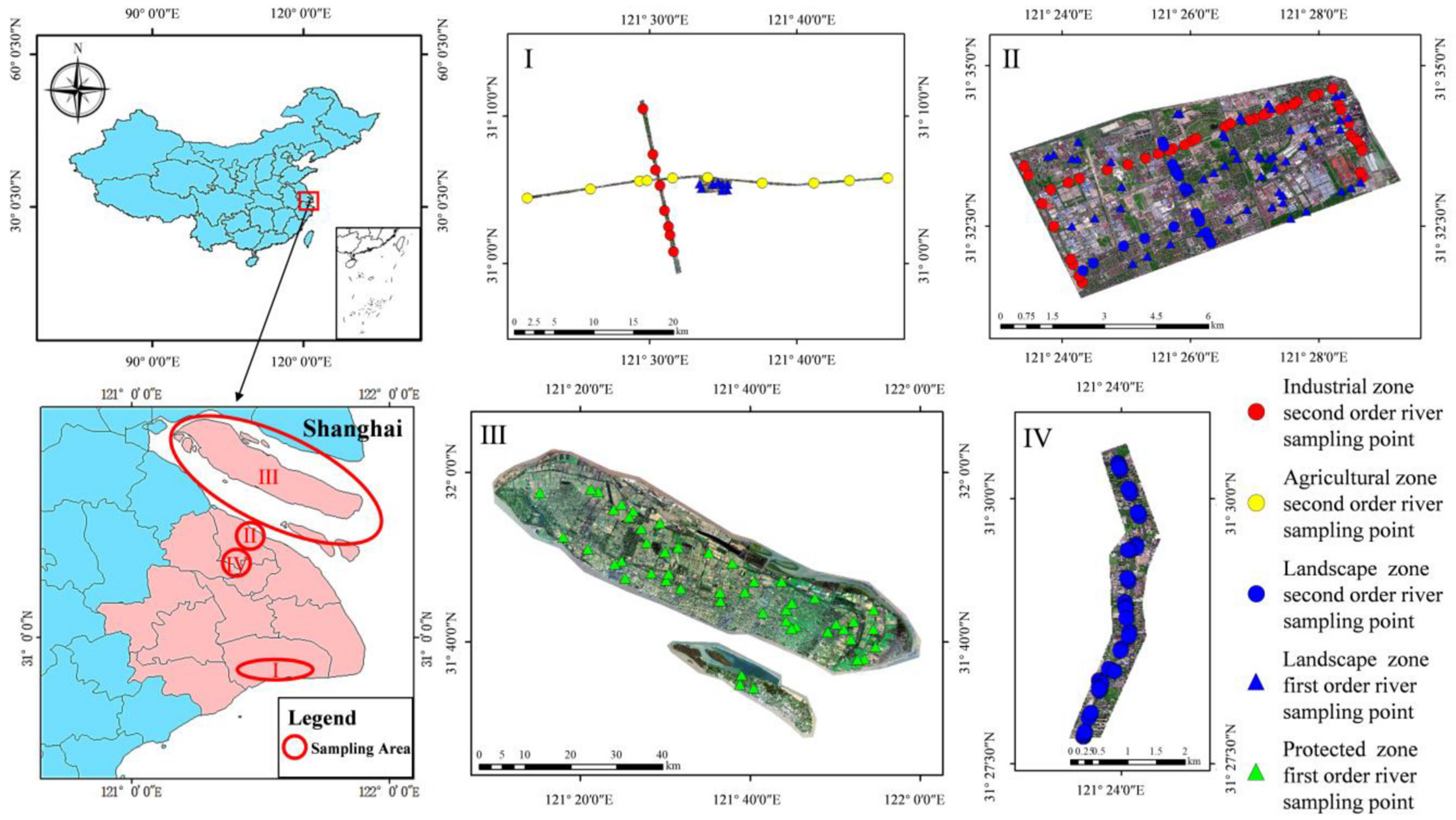
2.2. Data Collection and Site Description

2.2.1. In Situ Data Collection Method

Before applying water quality remote sensing, in situ data were needed to analyze the spectral features and spatial features. At each sampling point, the spectrum data and water quality samples were collected synchronously. Spectrum data were collected 5 times at the same sampling point.

The above-water measurement method [47,48] was used to collect the radiance and calculate the water reflectance. Using the following process, water reflectance can be calculated.

• Water-leaving radiance calculation:

$$L_w=L_{sw}-r\times L_{sky}$$

(1)

where $L_W$ is the water-leaving radiance.$L_{sw}$ is the total radiance signal received by the spectrometer above the water surface. $L_{sky}$ is the sky radiance. $r$ is operationally defined as the total sky-light actually reflected from the wave-roughened water surface in a certain direction divided by sky radiance, measured with the radiometer from direction.

• Downwelling incident irradiance calculation:

$$E_d\left(0^{+}\right)=L_p\times \pi /{\rho }_p$$

(2)

where $E_d\left(0^{+}\right)$ is the downwelling incident irradiance measured above the water surface. $L_p$ is the downward radiance measured with a standard reference panel. ${\rho }_p$ is the reflectance of the standard reference panel. In this paper, a white standard reference panel was used, the reflectance of which was 99%.

• Remote sensing reflectance calculation:

According to (1) and (2), the calculation equation of reflectance $Rrs$ can be obtained as follows:

$$Rrs=\frac{Lw}{E_d\left(0^{+}\right)}=\frac{L_{sw}-r\times L_{sky}}{L_p\times \pi /{\rho }_p}$$

(3)

According to the equations above, the reflectance of each band can be calculated and the reflectance curve can be obtained. The optical parameters above and the units are shown in (

Table A1. Optical parameter list.

Parameter	Parameter Symbol	Unit
Water-leaving radiance	$L_w$	μW/(cm2·nm·sr)
Sky radiance	$L_{sky}$	μW/(cm2·nm·sr)
Total radiance signal received by the spectrometer above the water surface	$L_{sw}$	μW/(cm2·nm·sr)
Downwelling incident irradiance	$E_d\left(0^{+}\right)$	μW/(cm2·nm)
Downward radiance measured with a standard reference panel	$L_p$	μW/(cm2·nm·sr)
Remote sensing reflectance	$Rrs$	Sr−1

. Since the spectrum data were collected 5 times, we were able to obtain 5 reflectance curves at one sampling point.

We chose total phosphorus (TP) and ammonia nitrogen (NH₃-N) as the water quality parameters for monitoring in our research. According to the People’s Republic of China’s national “Environmental Quality Standards for Surface Water” (GB3838-2002) [49], there are six grades of water quality (

Table 1. Water quality rankings.

Grade	TP (mg/L)	NH3-N (mg/L)
Grade I≤	0.02	0.15
Grade II≤	0.1	0.5
Grade III≤	0.2	1.0
Grade IV≤	0.3	1.5
Grade V≤	0.4	2.0
Worse than Grade V>	0.4	2.0

), with Grade I being the best. The ranking principle of the two water quality parameters in this paper is shown in Table 1.

The water quality parameters that need to be monitored are measured in the “State Key Laboratory of Pollution Control and Resource Reuse”. This laboratory passed the China Metrology Accreditation (CMA). The water samples were preserved in a freezer at four degrees Celsius. Both of the water quality parameters were measured within 2 days after the in situ sampling. TP was measured using a HACH DRB200 digital reactor block and a HACH DR2800 spectrophotometer using the digestion-ascorbic acid method. NH₃-N was measured using the HACH DR2800 spectrophotometer by means of Nessler‘s reagent colorimetric method.

The in situ sampling dataset needed to be representative. In this paper, four different condition requirements were considered: water quality diversity, water functional zone, stream order, and season.

Since urban rivers occupy complex situations, the samples needed to cover as many different and balanced types of water quality grades as possible to ensure that the samples were representative of the water conditions of the city. It was necessary to investigate the grade range of water quality parameters in the city. In addition, the distribution areas of rivers with different water quality grades also needed to be investigated. Then, sampling points were selected from these areas.

According to the “Functional Zoning of Water Environment in Shanghai” [50], the water functional zone can be divided into protected zones, landscape zones, industrial zones, and agricultural zones. The samples needed to cover all the water functional zones. According to the distribution areas of the water functional zone, sampling points were selected from these areas.

Stream order is based on Horton’s Law [51]. First-order stream segments are those that have no tributaries on a given map, and second-order stream segments are those that have as tributaries only first-order segments, etc. In urban areas, the width of first-order streams is usually less than 10 m, and they have very low velocity and flow, which means that they have a low hydrodynamic force and a low self-purification ability. Self-purification means the summary of all physical, chemical, and biological processes by which the quantity of the pollution in the stream is decreased. Second-order streams and higher-order streams have greater flows and higher velocities. The samples needed to cover different stream orders.

Season can affect the growth of microorganisms and algae, which can indirectly influence the water’s color. Additionally, season is an important factor that affects water quality in East China [52,53]. Thus, in different quarters of a year, different samples needed to be collected to enrich the dataset.

Water quality grade, water functional zone, stream order, and season were combined with samples. Therefore, each sample had 5 reflectance curves, the concentration value of water quality parameters, and the data of four conditions.

2.2.2. Composition of the Dataset

The dataset was collected in Shanghai, China, which is a megacity with more than 43,000 waterways. Shanghai has a complete water functional zone system, which includes protected zones, landscape zones, industrial zones, and agricultural zones. The water quality in Shanghai is diverse. In the protected zone, the water quality is better than that in the other areas. However, in the living and working areas where human activities are intensive, the water quality is usually worse.

From 13 June 2018 to 14 May 2019, we collected samples from 236 sampling points in different places throughout Shanghai (Figure 1). These points were distributed in Chongming District, Baoshan District, Fengxian District, and Putuo District. According to the sampling condition requirements, the sample dataset covered all types of water functional zones in Shanghai. The rivers in Shanghai can be mainly divided into four stream orders. In this dataset, stream orders included the first to the second order. The third- and fourth-order rivers were not covered in this dataset, because they are too long and wide for UAV remote sensing. Moreover, they are monitored continuously by the Shanghai Water Authority. The grades of the TP samples covered from grade II to worse than grade V. The grades of NH₃-N samples covered from grade I to worse than grade V. The proportions of different requirements in the dataset are shown in Figure 2.

2.2.3. UAV-Borne Multispectral Water Quality Remote Sensing Application Process

In the application of UAV-borne multispectral remote sensing water quality monitoring, we propose a process that is practical. The data collection process mainly includes image collection, ground radiance collection, and checkpoint collection.

Remote sensing image collection follows the rules of traditional aerial photogrammetry. For a large area that cannot be covered within one flight, multiple flights are planned to cover the whole area. To improve the signal–noise ratio of the image and avoid the specular reflection of the river water, the solar elevation angle should be between 35° and 65° during the collection of the images [54].

Remote sensing images of the ground and solar radiance are collected simultaneously. A 99% standard reference panel and the same multispectral camera is used on the UAV to collect the downward radiance. The two cameras are calibrated by the same calibration equipment. Both the images and solar radiance data use the GPS (global positioning system) timing system. The solar radiance curve can be obtained by cubic spline interpolation. This curve can be used as a reference for relative radiometric correction and downwelling incident irradiance $E_d\left(0^{+}\right)$ calculations.

Water quality samples are taken as the checkpoints when the UAV is flying directly above. The samples are analyzed in the laboratory.

Before using the water quality grading model to classify the grades of the rivers, it is necessary to perform image pretreatment. The first step is image correction, which includes geometric correction [55,56,57], absolute radiometric correction [58,59,60], and relative radiometric correction [61,62,63] using conventional multispectral camera-calibration methods. After image fusion, each image has multiple channels: RGB channels and multispectral channels.

After image correction, the ground radiance from the images can be obtained directly. The average value of 9 pixels in the center of the image is taken as the downward radiance. With the downwelling incident irradiance$E_d\left(0^{+}\right)$ measured above the water surface calculation and Equation (3), the images that contain the reflectance values can be obtained.

The orthophoto map is established in advance. Then, the river area image is manually clipped from the orthophoto map. This river area image contains the reflectance value channels.

2.2.4. Study Site

The study site in this research was located in Yanghang town, Baoshan District, Shanghai, which has a complex river network. The experimental area covers an area of 13.6 square kilometers. This area is mainly used for residential and industrial production. There are 16 rivers, including 13 first-order streams and 3 second-order streams. Two of the second-order streams, called the Beisitang River and the Meipu River, are mainly used for industry and are canals. Another second-order river, called the Yangsheng River, is a river used as a landscape feature. Furthermore, first-order rivers are mainly used as landscape rivers. The total length of the rivers is 20.0 km. Because of the effect of human activities, sewage pollution makes the water quality here poor.

To cover the whole area by UAV, it took 3 days, from 4 September 2018 to 6 September 2018, to complete a total of 16 flight–ground observation and spectral data-collection tasks. The average area of a single flight was 0.85 square kilometers. The flight height was 300 m. The forward overlap and side overlap were both 80% to ensure that there was enough overlap between the two flights in the process of establishing the orthophoto map. Additionally, there was an overlapping route between two adjacent flights. The overlap was 80%. The total number of images was approximately 7000. During each flight, another multispectral array camera was used to collect downward radiance. The camera took a group of images every three seconds.

Fifteen checkpoints were collected to compare the results of the models. The study site, flight zoning, river condition, and checkpoints are shown in Figure 3.

2.3. Feature Analysis for Urban River Water Quality Remote Sensing

Feature analysis was carried out based on the in situ dataset. The results can provide a band group scheme for the multispectral sensor. Spectrum and space were two key features used in this study. Spectral feature analysis was divided into 3 parts: spectral information analysis, correlation analysis between the spectrum and water quality parameters, and bandwidth analysis. Spatial feature analysis used kernel canonical correlation analysis (KCCA) to prove that spatial features can improve the model grading accuracy.

2.3.1. Spectral Features Analysis

Dimensionality reduction is a common method for selecting spectral features. Factor analysis can find hidden and representative factors in many variables. The number of variables can be reduced by grouping variables of the same essence into several factors.

A screening test was used to determine the number of factors that need to be grouped. The in situ reflectance dataset was set as a two-dimensional matrix $X_{n*p}$ ($n$ is the number of samples, and $p$ is the number of measured bands). Then, the correlation coefficient matrix of the reflectance dataset was calculated. By calculating the correlation coefficient of every two bands, a correlation coefficient matrix $R_{p\ast p}$ was obtained. ${\mathsf{\lambda }}_i$ (${\mathsf{\lambda }}_{1 },{\mathsf{\lambda }}_2, {\mathsf{\lambda }}_3,\dots \dots , {\mathsf{\lambda }}_p>0$) are the eigenvalues of $R_{p\ast p}$. Usually, we chose the number of eigenvalues larger than 1 as the number of grouped factors [64].

With the factor-loading matrix analysis, the relationship between the factor variables and the reflectance data was obtained. Varimax orthogonal rotation was used to make the original factor variables more interpretable. After the rotation, a factor rotation component matrix was obtained, which provided the contribution rates of each band for different factors. Then, the contribution rates of each factor were normalized to the range of 0 to 1. We took the normalized rates that were larger than 0.90 as the possible spectral feature band ranges [65].

For water quality remote sensing, not only should the information of the spectrum itself be analyzed, but the correlation between the spectrum and water quality parameters also needs to be taken into consideration. Different parameters usually have different spectral features.

Correlation analysis was used to calculate the correlation coefficient between the reflectance ratio of each pair of bands and the contribution of each water quality parameter. Furthermore, all the correlation coefficients were normalized to the range of 0 to 1. We took the normalized coefficients that were larger than 0.90 [65] as the possible spectral feature band ranges.

Finally, we obtained the union of all the possible spectral feature band ranges of each method as the center wavelength. Spectral feature bands identified by different methods were assigned a higher priority. If at least 2 methods chose the same feature, this then became the high-priority band for the multispectral sensor.

Spectral resolution is a significant index for remote sensing that can affect the observation accuracy. For water quality, a more accurate measurement of water reflectance means better grading results were obtained.

One band was selected from the spectral feature band ranges. The reflectance of this band in the dataset was set to be the accurate reflectance value. Taking this band as the central wavelength, the bandwidth continued to expand from 0 to the left and right sides. Each time, the bandwidth expanded 2 nm. After expanding the bandwidth, Equation (3) was used to calculate the new reflectance. $E_d\left(0^{+}\right)$ and $L_w$ are the total of the downwelling incident irradiance measured above the water surface and the water-leaving radiance from the left side to the right side of the bandwidth. The absolute percent difference (APD) was used to compare the accurate reflectance value and new reflectance value.

$$APD=\frac{\sqrt{{{\displaystyle \sum }}_{i=1}^n{\left(Rr{s}^{acc}\left(i\right)-Rr{s}^{new}\left(i\right)\right)}^2}}{{{\displaystyle \sum }}_{i=1}^{n}Rr{s}^{acc}\left(i\right)}$$

(4)

where $n$ is the number of samples. $Rr{s}^{acc}$ is the accurate reflectance value. $Rr{s}^{new}$ is the new reflectance value. Then, the curve of bandwidth and the $APD$ were obtained. The method that was used to determine the bandwidth demonstrated that the $APD$ was within 0.25% [18].

2.3.2. Spatial Features Analysis

By introducing spatial features, interclass separability should be improved. In this study, we considered the water functional zone and stream order. Usually, the correlation between spectral features and the water quality parameters was not linear, instead being nonlinear. Thus, we used KCCA to verify the improvement after using the spatial features.

KCCA introduces the kernel function into a canonical correlation analysis (CCA) [66]. This method maps low-dimensional data to a high-dimensional feature space, which makes the correlation analysis in the kernel function space convenient. For the water quality parameter concentration and reflectance of spectral feature bands, we obtained the following equations:

$$u=w_C^T{\Phi }_C\left(C\right)$$

(5)

$$v=w_X^T{\Phi }_X\left(X\right)$$

(6)

where $C$ is the water quality parameter concentration matrix. $X$ is the reflectance matrix of spectral feature bands. ${\Phi }_C$ and ${\Phi }_X$ are the kernel functions. The radial basis function (RBF) is used as the kernel function in this paper. $w_C^T$ and $w_X^T$ are the coefficients of the linear combination $u$ and $v$. The aim is to find $w_C^T$ and $w_X^T$, which can make the correlation coefficient of $u$ and $v$ the highest. Under the restriction of spatial features, the result of KCCA should be better than the result produced without using spatial features.

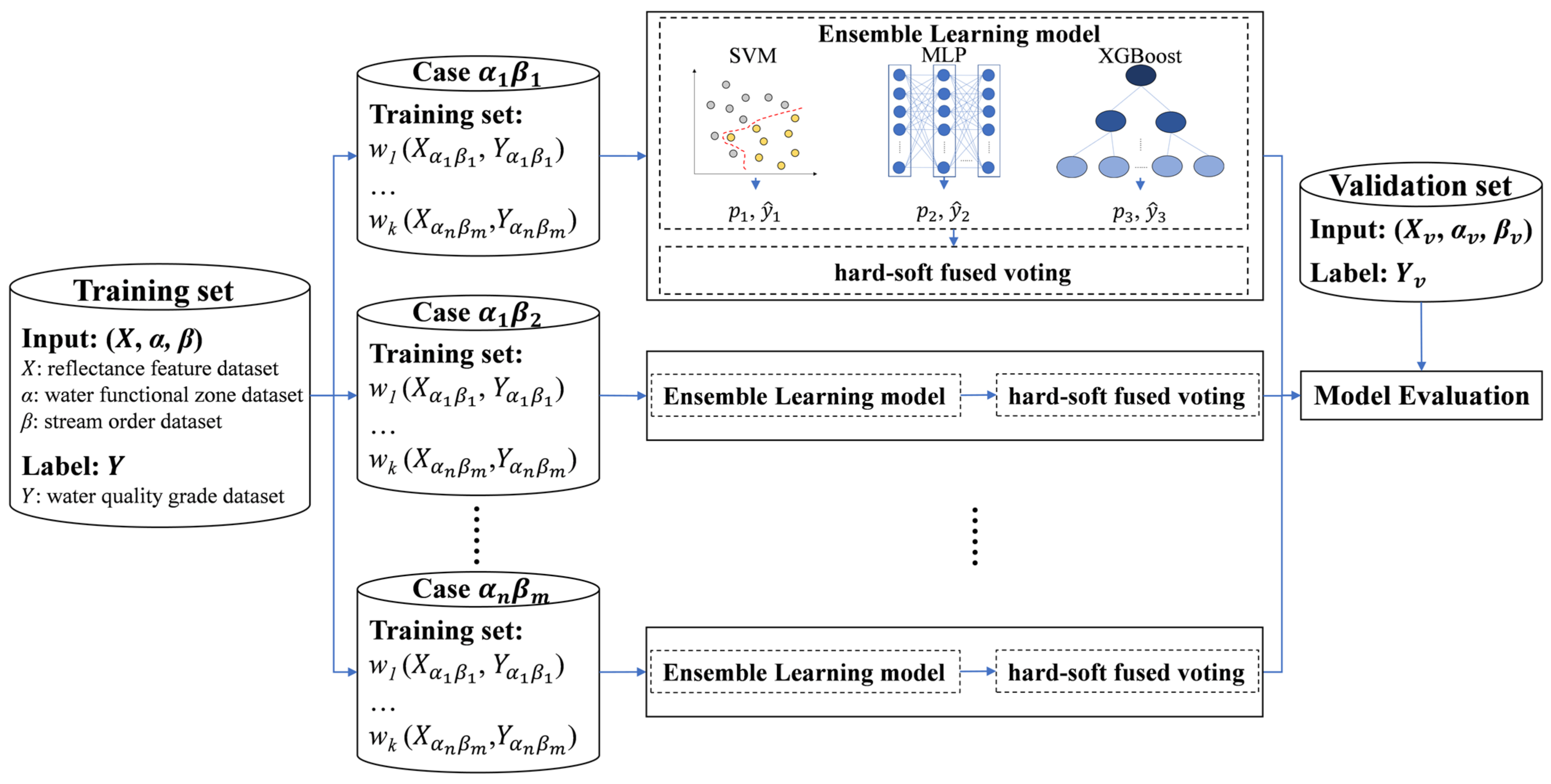
2.4. Spectral- and Spatial-Feature-Integrated Ensemble Learning

For remote sensing water quality grading, a spectral- and spatial-feature-integrated ensemble learning method was proposed. Samples were divided into different training sets according to the spatial features. Under the restriction of different spatial features, training sets were given different weights to be trained. A hard-soft fused voting method was used to obtain the final grading result.

2.4.1. Ensemble Learning Model

For the ensemble learning method (Figure 4), three machine-learning-based techniques were applied: support vector machine (SVM), multilayer perceptron (MLP), and extreme gradient boosting (XGBoost).

The reflectance feature dataset $X$ was integrated with the spatial feature dataset ($\alpha , \beta$) as the model input. According to the spatial features, which were the water functional zone condition (${\alpha }_1$, ${\alpha }_2$, ……, ${\alpha }_n$) and stream order condition (${\beta }_1$, ${\beta }_2$, ……, ${\beta }_m$), the reflectance feature dataset $X$ was divided into different training sets ($X_{{\alpha }_1{\beta }_1}$, $X_{{\alpha }_1{\beta }_2}$, ……, $X_{{\alpha }_2{\beta }_1}$, $X_{{\alpha }_2{\beta }_2}$, ……, $X_{{\alpha }_n{\beta }_m}$). The $n$ and $m$ are numbers of different spatial feature types. Different weights $W$ were given to the training set. Under the restriction of different spatial conditions, the weight $W$ was different.

SVM is a classifier with sparsity and robustness that can use hyperplanes to perform nonlinear classifications. SVM has been successfully utilized in remote sensing water quality inversion [34]. The optimal kernel function, slack variable, penalty parameter, and gamma coefficient was selected to construct a hyperplane. The penalty parameter followed the classification optimization problems below:

$$\min \frac{1}{2}\left|\left|w\right|\right|+C{\displaystyle \sum }_{i=1}^i{\xi }_i$$

(7)

$$s.t. y_i\left[\left(w{x}_i\right)+b\right]\ge 1-{\xi }_i \left(i=1, 2,\dots \dots ,n\right)\left({\xi }_i\ge 0\right)$$

(8)

where $w$ is the coefficient of the hyperplane equation. $\xi$ is the slack variable, which is the allowed amount of deviation from the functional margin for the corresponding training data points. $C$ is the penalty parameter. When using kernel functions of ‘RBF’, ‘poly’, and ‘sigmoid’, the gamma coefficient needs to be optimized. The equation of the gamma coefficient is as follows:

$$gamma=\frac{1}{2\times {\sigma }^2}$$

(9)

where $\sigma$ is the standard deviation parameter in the normal distribution.

MLP is a multilayer neural network that contains a single input layer, multiple hidden layers, and one output layer. For water quality inversion, neural networks have shown promising results by generating high overall model accuracies [9]. A single hidden layer neural network can be written as the equations below:

$$H=\Phi \left(X{W}_h+b_h\right)$$

(10)

$$O=softmax\left(H{W}_o+b_o\right)$$

(11)

where $X$ denotes the samples. $\Phi$is the activation function. $W_h$ and $W_o$ are the weights of the hidden layer and output layer, respectively. $b_h$ and $b_o$ are the biases of the hidden layer and output layer, respectively. $O$ is the output value. The softmax function is used to map the output to (0,1), which indicates the classification probability.

XGBoost, which is a tree boosting system, implements the gradient-boosting decision tree (GBDT) efficiently, and many improvements are made in this system. This system is widely used by data scientists and provides state-of-the-art results for many problems [67]. Additionally, it has been successfully used in water quality monitoring [68]. In the general case, the objective function, which consists of two parts (training loss and regularization term) can be transformed into the equation below:

$$ob{j}^{\left(t\right)}={\displaystyle \sum }_{i=1}^{n}l\left(y_i,{\widehat{y}}_i^{\left(t-1\right)}+f_t\left(x_i\right)\right)+\mathsf{\Omega }\left(f_t\right)+c$$

(12)

where $l$ is the loss function and $\mathsf{\Omega }$ is the regularization function. $n$ is the number of samples. $y$ is the label value, and $\widehat{y}$ is the model predictive value. $t$ is the step number of model prediction. $f$ is the tree function, which contains the structure of the tree and the leaf scores. $x$ is the sample value. $c$ is the constant.

Each classifier can output three groups of possibilities ($P$ ([$p_1, p_2, p_3$])) and the grading results ($\widehat{Y}$ ([${\widehat{y}}_1, {\widehat{y}}_2, {\widehat{y}}_3$])). The possibility of each classifier has six possible values according to the six water quality parameter grades.

A hard-soft fused voting method was used to obtain the final grading result. If the three grading results of the classifiers were the same or two of the results were the same, the hard-voting strategy was used. In addition, an improved soft-voting strategy was used. The voting method is shown below:

$$\left\{\begin{array}{c}Index\left(Max\left(A{P}^T\right)\right) if {\widehat{y}}_1\ne {\widehat{y}}_2\ne {\widehat{y}}_3\\ Mode\left(\widehat{Y}\right) if else\end{array}\right.$$

(13)

where $Index$ is the method, which obtains the index of a certain value. $Max$ means the method that obtains the largest value of a list. $A$ is the accuracy array of the three classifiers. $Mode$ indicates the method, which obtains the mode of a list.

2.4.2. Model Evaluation

Five-fold cross validation was used to validate the models. The results of SVM, MLP, XGBoost, and the ensemble learning method using traditional spectral features, and the results of SVM, MLP, XGBoost, and the ensemble learning method using spectral and spatial features were compared. Five-fold cross validation was used to validate the models.

Precision, recall, and F1 scores were used to evaluate the results. For multiclassification, the macro average is a common strategy to evaluate the models [69,70]. The model evaluation indexes and the calculation formulas are shown in

Table 2. Evaluation indexes for water quality grading model.

Evaluation Index	Calculation Formula
Precision	$\frac{TP}{TP+FP}$
Recall	$\frac{TP}{TP+FN}$
F1 score	$2\times \frac{Precision\times Recall}{Precision+Recall}$
Macro Precision	$\frac{1}{n}{\displaystyle {\displaystyle \sum }_{i=1}^n}Precisio{n}_i$
Macro Recall	$\frac{1}{n}{\displaystyle {\displaystyle \sum }_{i=1}^n}Recal{l}_i$
Macro F1 score	$\frac{1}{n}{\displaystyle {\displaystyle \sum }_{i=1}^n}F{1}_i$

Where $TP$ denotes true positive, $FP$ denotes false positive, $FN$ denotes false negative, $F1$ denotes the F1 score, and $n$ denotes the number of grades.

.

3. Results

3.1. Feature Analysis Results for Urban River Water Quality Remote Sensing

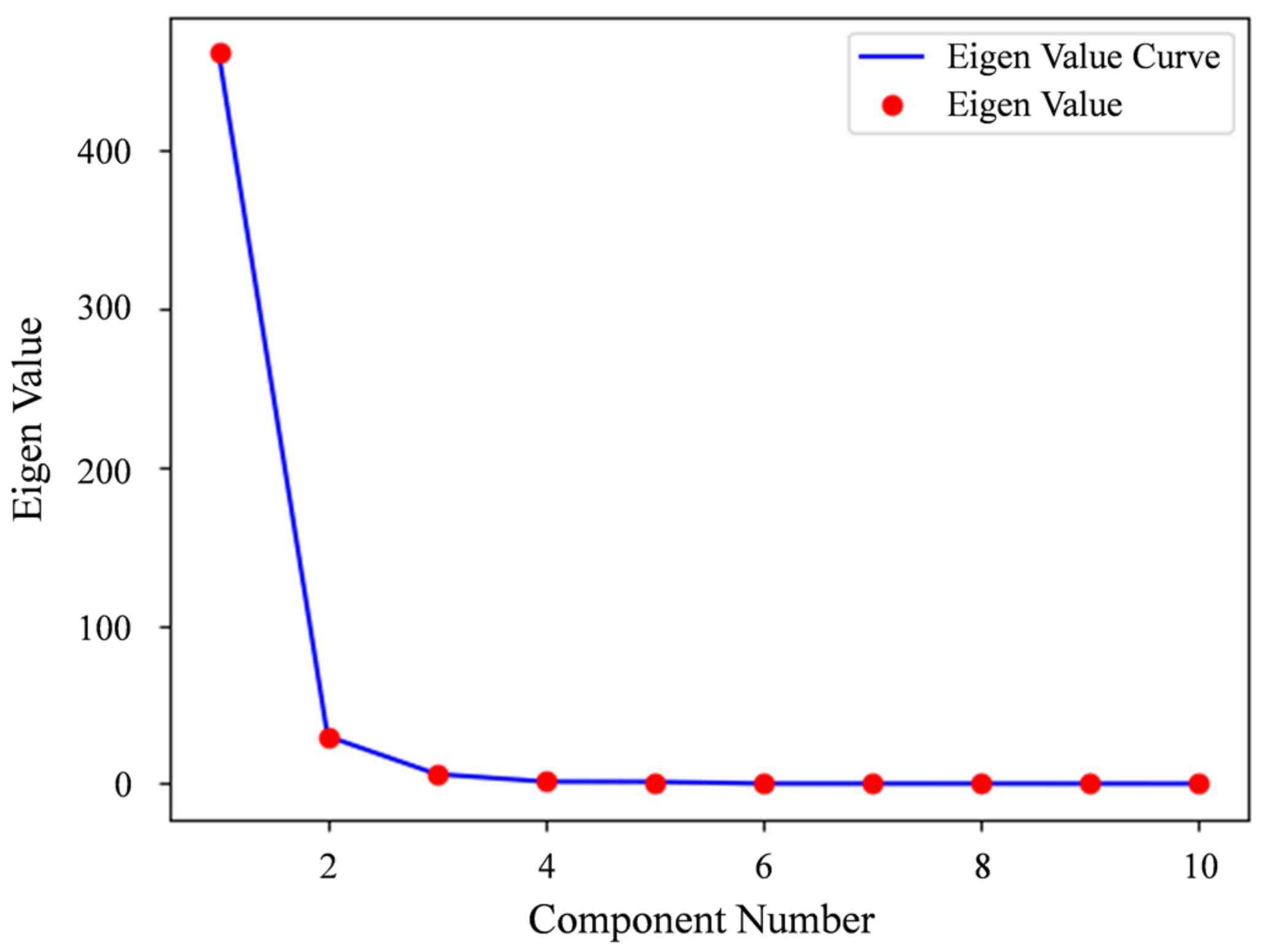
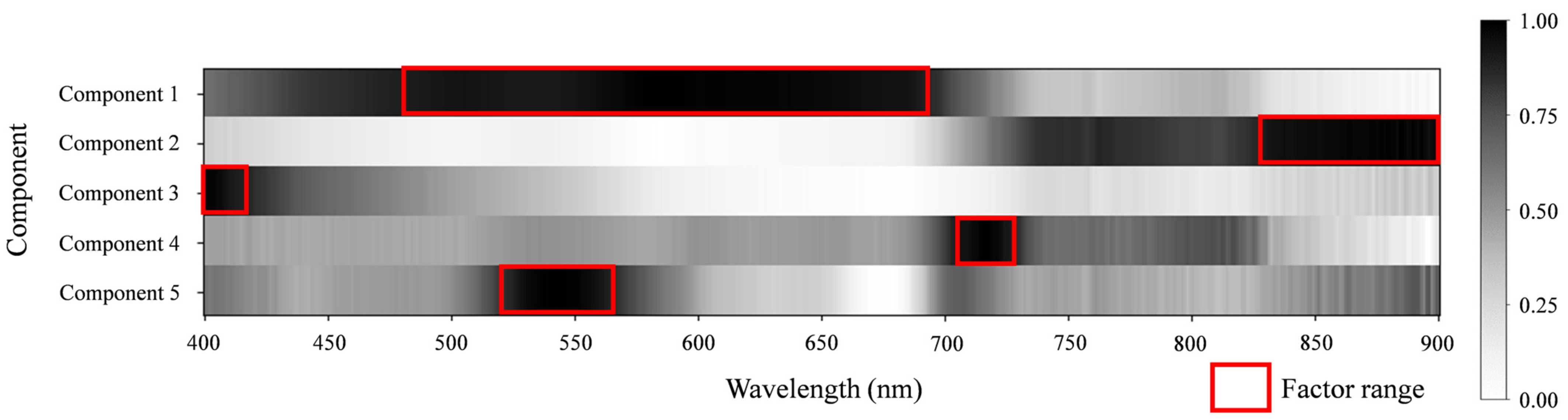
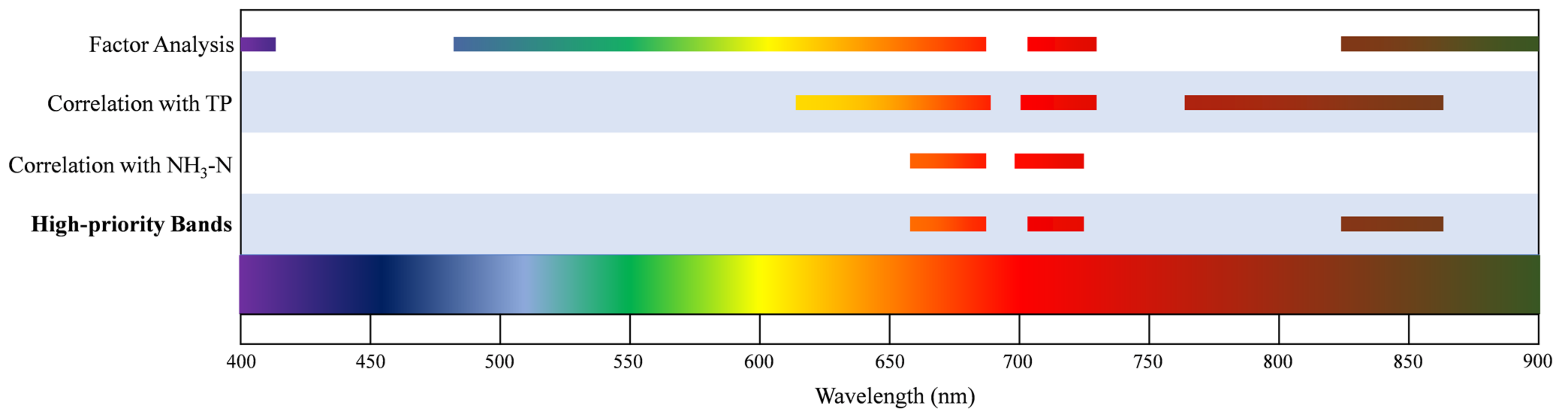
3.1.1. Spectral Feature Analysis

The spectral feature analysis was based on the reflectance dataset collected before the application of the experiment. The purpose was to determine the bands used on the multispectral array camera. A scree test was used to choose the numbers of bands that needed to be extracted. The scree plot is shown in Figure 5. Among all eigenvalues, five values were larger than 1, which were 460.96, 29.95, 6.10, 1.37, and 1.23. Thus, the number of grouped factors was five. Then, factor analysis was used to select the spectral features. The results of the five different components that were normalized are shown in Figure 6. The main contribution to the wavelength area of factor 1 was from 483 to 690 nm, which corresponds to the largest eigenvalue. Those of the other four factors were from 829 to 900 nm, from 400 to 413 nm, from 705 to 726 nm, and from 526 to 562 nm. Hence, the green band, infrared band, blue band, and red band were the most important factors for representing the river reflectance.

The correlation between the spectrum band ratio and water quality parameters of the sampling dataset was analyzed to select the feature bands for the TP and NH₃-N grading models. The original results are shown in Figure 7. The largest correlation coefficient between the spectrum and TP was 0.52. For NH₃-N, the value was 0.53. Both values were too low, which means that they were not suitable for using linear regression to grade the water quality. To choose the feature band ranges, the results were normalized, as is presented in Figure 8. For TP, at approximately 820/650 nm and 710/650 nm, the normalized correlation coefficients were larger than 0.90. For NH₃-N, at approximately 710/675 nm, the normalized correlation coefficients were larger than 0.90.

Figure 9 shows the final selected bands. The resulting unions were from 400 to 413 nm, from 483 to 693 nm, 698–726 nm, and 790–900 nm, which were the possible center wavelength ranges for the multispectral sensor. The high-priority center wavelength ranges were at the results’ intersection, namely at 655–690 nm, 705–721 nm, and 829–861 nm. These wavelength ranges are the final bands that are used on the homemade narrowband multispectral array camera in this paper.

To determine the bandwidth of each selected band, the $APD$ between the reflectance of the center wavelength and reflectance of different bandwidths was calculated. In general, the $APD$ increases with increasing bandwidth, and the $APD$ is wavelength-dependent. The $APD$ values for the bands on the homemade camera are shown in Figure 10. For 675, 705, and 850 nm, the bandwidth needed to be narrower than 42, 34, and 18 nm, respectively, as shown in Figure 10. For the homemade camera, 10 nm was chosen as the bandwidth of all the bands, which was suitable according to the results.

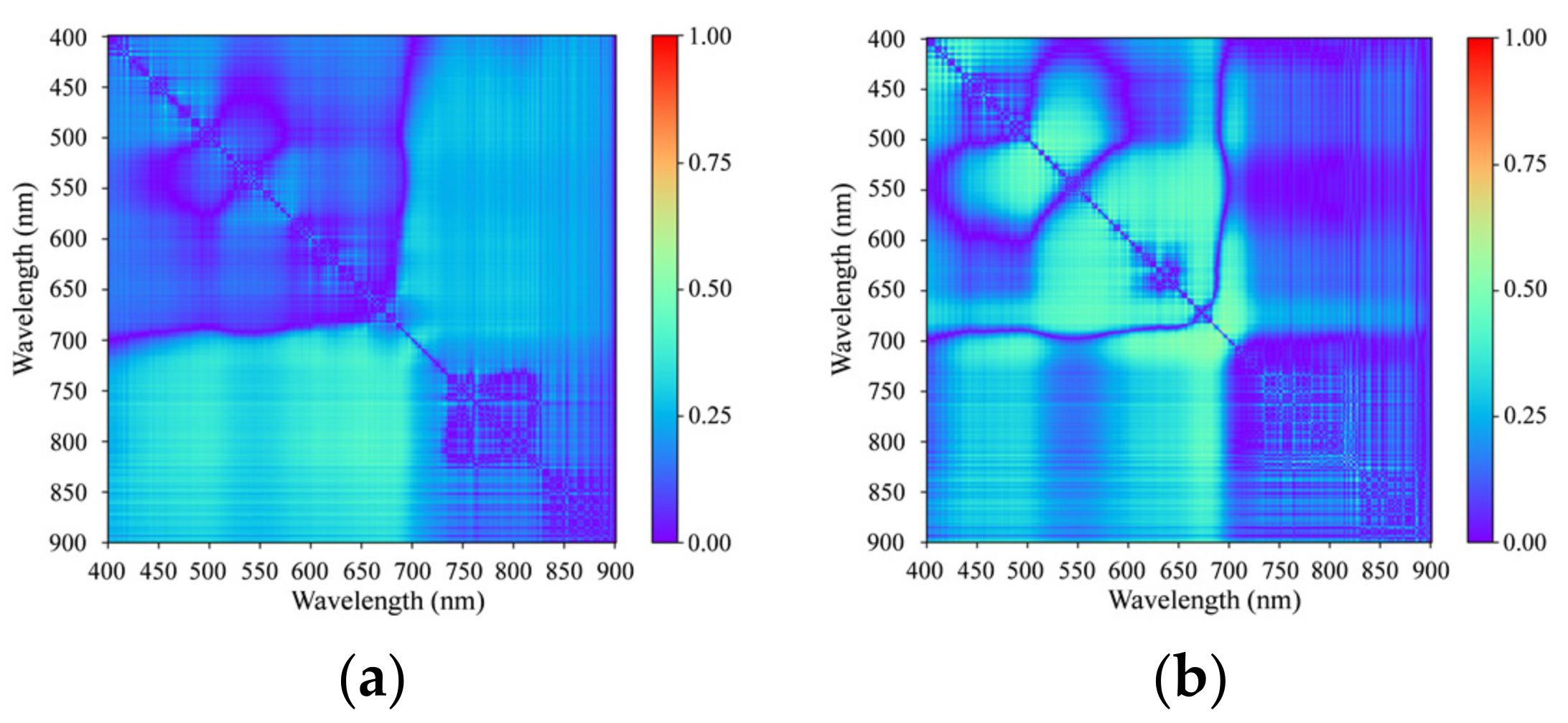
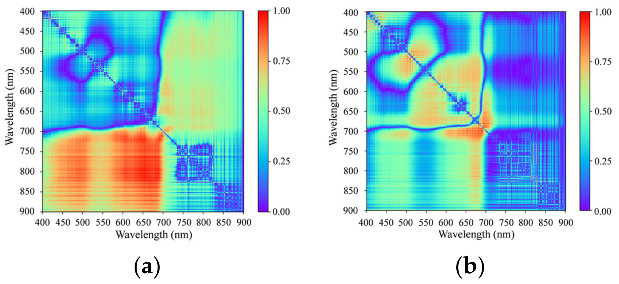
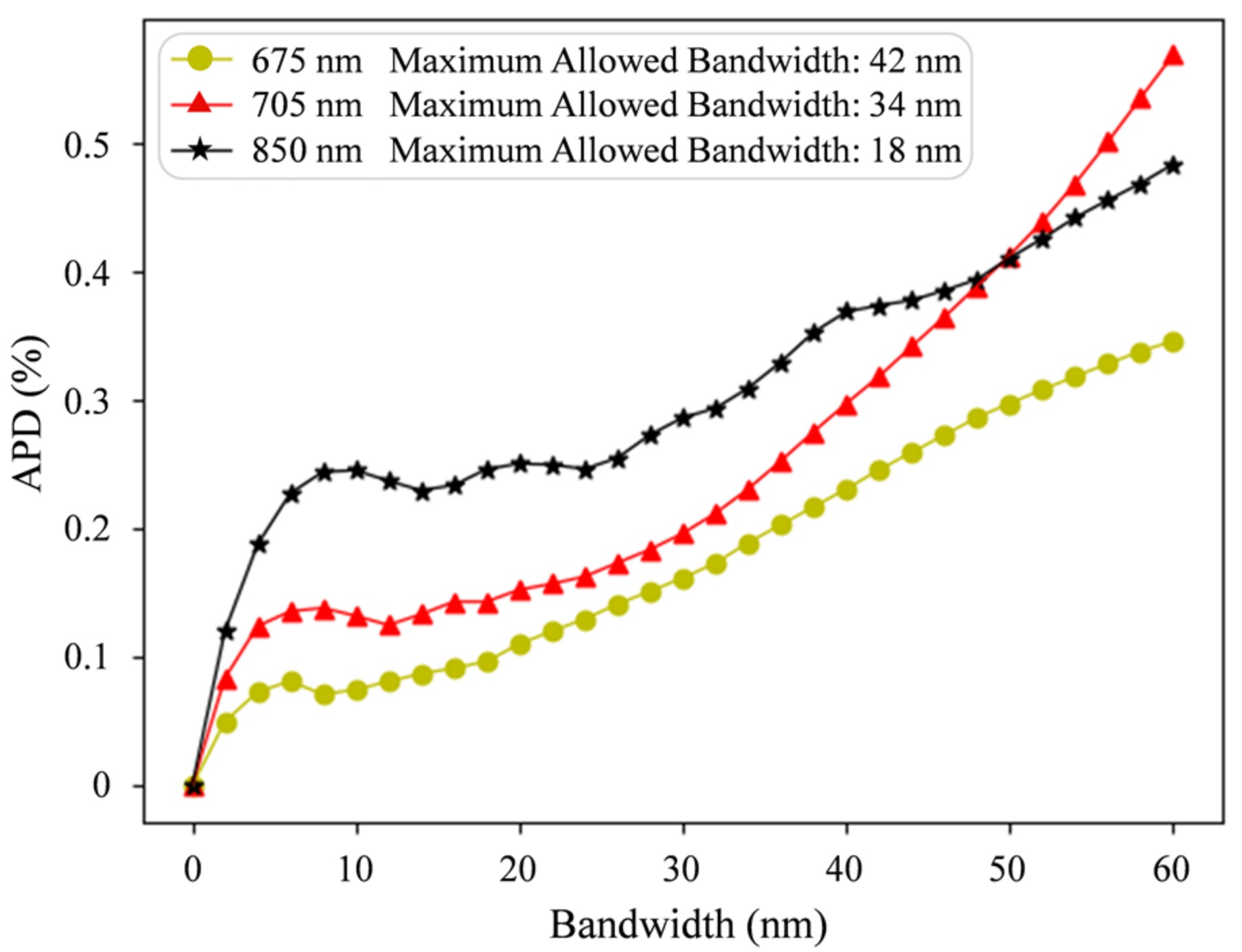
3.1.2. Spatial Feature Analysis

In this paper, the dataset was divided into four different training sets according to the recorded spatial feature of each sampling point: protected zone first-order stream, landscape zone first-order stream, landscape zone second-order stream, and industrial and agricultural zone second-order stream. The industrial zone and agricultural zone were combined because there were too few of each of them to be a training set. Thus, they were combined to balance the sampling quantity of each training set.

The RBF was used as the kernel function in this paper. For each training set, the kernel canonical correlation coefficients between TP and NH₃-N concentrations and spectral-feature reflectance were calculated. The results are shown in

Table 3. Kernel canonical correlation coefficients between water quality parameters concentration and spectral-feature reflectance.

Case	TP	NH3-N
Original dataset	0.66	0.68
First-order stream of protected zone	0.71	0.75
First-order stream of landscape zone	0.68	0.85
Second-order stream of industrial and agricultural zone	0.76	0.83
Second-order stream of landscape zone	0.68	0.79

. All the correlation coefficients of the training set using spatial features were larger than the correlation coefficients of the original dataset, which means that, upon introducing spatial features, the water quality parameters had a better interclass separability.

3.2. Modeling Results

In this section, eight different models are compared. Four of the models were SVM, MLP, XGBoost, and ensemble learning with only spectral features. The other four models were SVM, MLP, XGBoost, and ensemble learning with spectral and spatial features. The data of 236 sampling points were used to train and evaluate the models. Five-fold cross validation was used to evaluate all the models. Each fold used macro precision, macro recall, and macro F1 scores as the basis of evaluation.

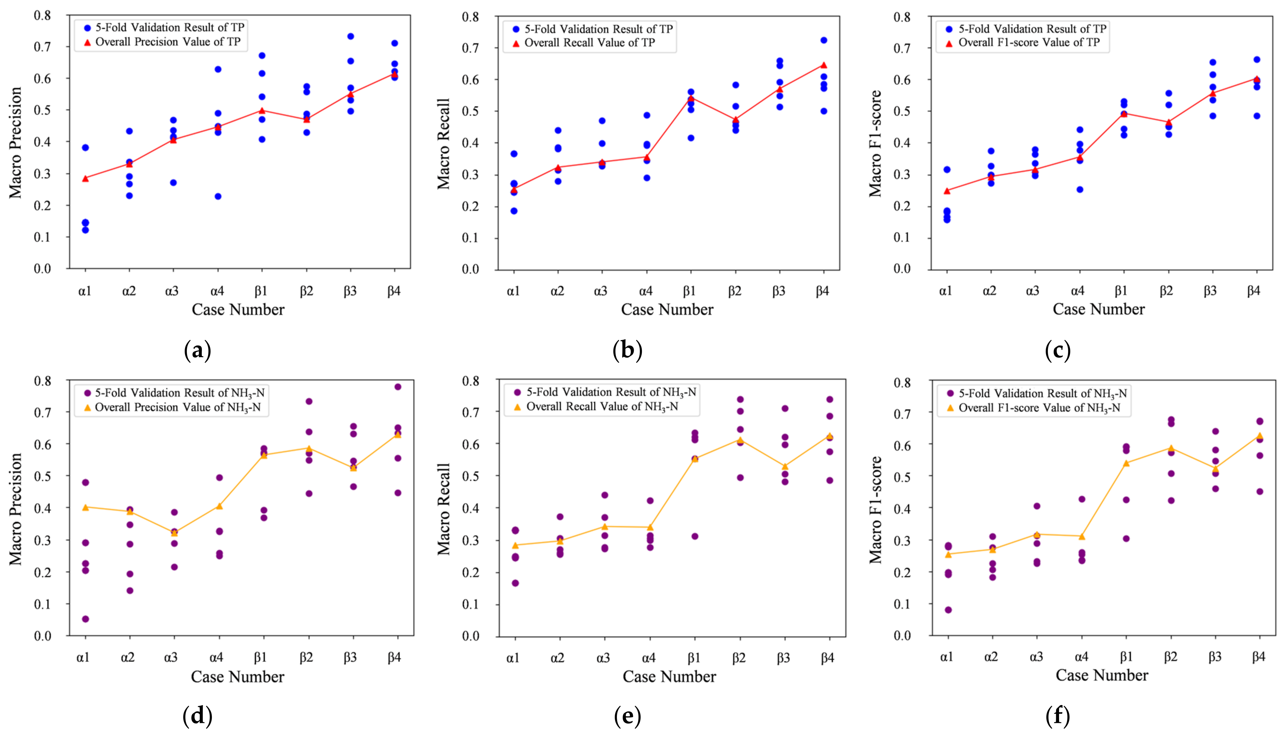
3.2.1. Results of Models Using Spectral Features

The grading models for TP and NH₃-N using only spectral features generated relatively low macro precision, macro recall, and macro F1 scores, which were not suitable for urban river water quality remote sensing (Figure 11). SVM showed the worst results for TP grading, which was only approximately 0.25 for the three kinds of evaluation values. MLP was relatively better than SVM. However, the evaluation values were all lower than 0.35. The macro precision of XGBoost was 0.41, but the other values were lower than 0.4. Ensemble learning produced the best TP grading results. However, the three values were 0.45, 0.36, and 0.36, which were also low.

SVM showed the worst recall and F1 scores for NH₃-N grading, which were 0.28 and 0.25, respectively. XGBoost showed the worst precision, which was 0.32. According to recall and F1 scores, XGBoost performed slightly better than SVM and MLP. However, the evaluation values were still around 0.35. The recall and F1 scores of ensemble learning were a slightly lower than XGBoost; however, precision was the highest among the four models.

The three machine-learning models were all worse than the ensemble learning model, whether for TP or NH₃-N, which indicates that the ensemble learning model had a higher classification accuracy than the single machine-learning model. Nevertheless, all the models using only spectral features are not suitable for urban water quality monitoring due to the low accuracy.

3.2.2. Results of Models Using Spectral and Spatial Features

Compared to the results of models using only spectral features, the accuracy of all models improved using spectral and spatial features (Figure 11). For TP grading, XGBoost had the greatest macro precision, macro recall, and macro F1 score improvement among the three traditional machine-learning models, which improved from approximately 0.35 to more than 0.55. The evaluation values of MLP and XGBoost both increased to approximately 0.50. Ensemble learning using spectral and spatial features performed best for TP grading. The macro precision, macro recall, and macro F1 scores were 0.61, 0.65, and 0.60, respectively.

MLP was the best model for NH₃-N grading among SVM, MLP, and XGBoost. The evaluation values were approximately 0.60. SVM showed similar results, which were slightly lower than those of MLP. XGBoost showed the worst result. The macro precision, macro recall, and macro F1 scores were just around 0.50. The evaluation values of the three machine-learning models all increased by at least 0.2 with the introduction of spatial features. Likewise, the ensemble learning model had the best training results. The macro precision, macro recall, and macro F1 scores were 0.63, 0.62, and 0.63, respectively.

From Figure 11, we can obviously find that when using both spectral and spatial features, the water quality classification ability of the machine-learning models improved dramatically. Moreover, despite the worse-than-grade Ⅴ TP, all the other grading accuracies were larger than 0.50 (Figure 12). Both ensemble learning models for TP and NH₃-N grading performed the best among all the grading models and were applied to the experiment in Yanghang town.

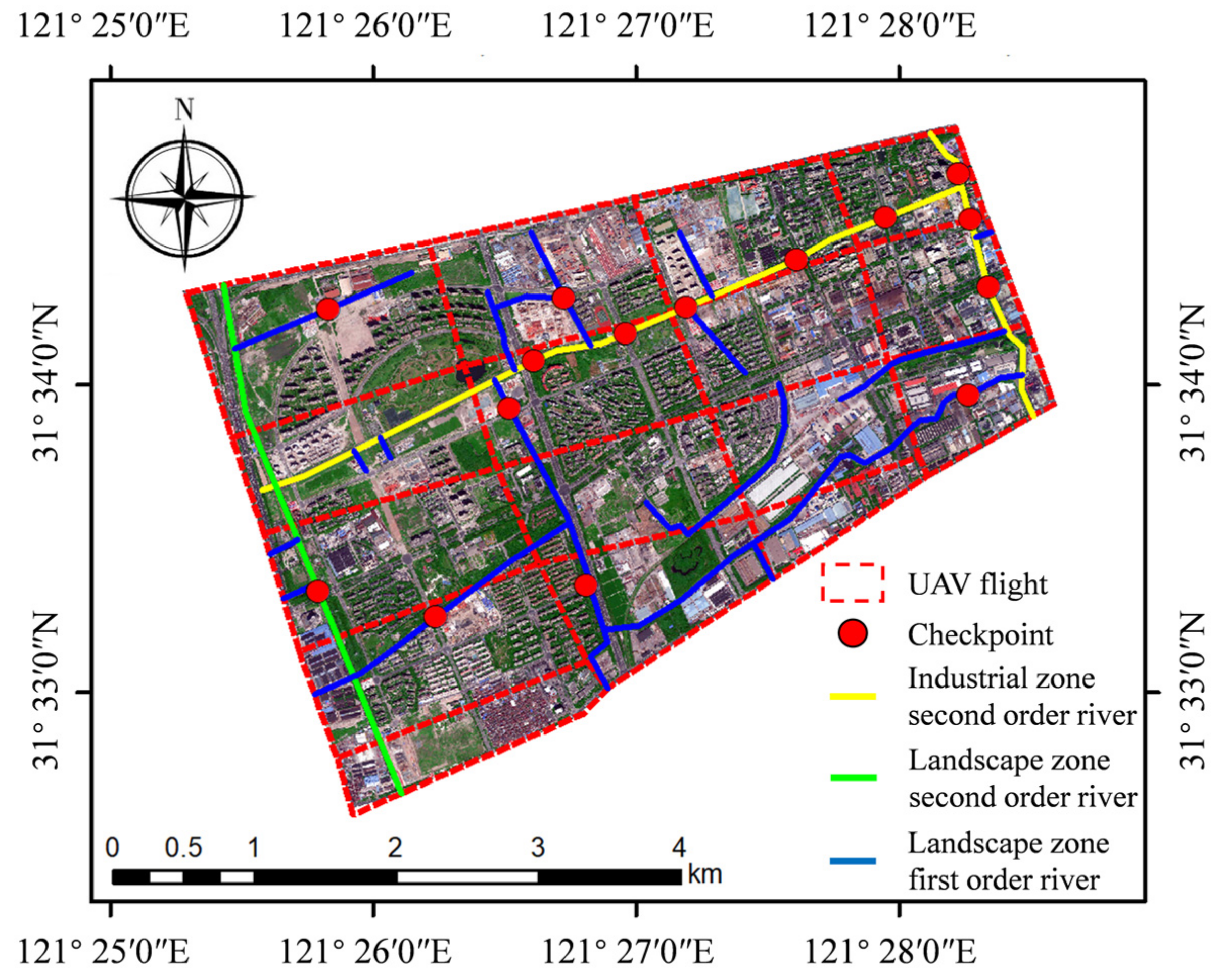
3.3. Application Experiment Results

The UAV-borne multispectral remote sensing water quality monitoring application experiment was performed from 4 September 2018 to 6 September 2018 in Yanghang Town, Baoshan District, Shanghai. Geometric correction, absolute radiometric correction, and relative radiometric correction was carried out to obtain the ground radiance. The standard reference panel images collected by the camera on the ground were used to generate the downward radiance interpolation curves. With the corrected remote sensing images and curves, the reflectance of the rivers was obtained. Considering the influence of different spatial factors of the rivers, ensemble learning models using spectral and spatial features were used to grade the water quality. Finally, water quality grading maps of TP and NH₃-N in Yanghang town were drawn.

3.3.1. Image Data Preprocessing

The remote sensing images and standard reference panel images were first corrected and fused. After these processes, each image had six channels: R, G, B, 675, 705, and 850 nm. The pixel values of multispectral channels had a functional mapping with radiance.

Each flight had a group of downward radiance values obeying the GPS timing system. With the radiance curves and corrected remote sensing images, the pixel values of multispectral channels were transformed to values that had a functional mapping with reflectance.

A PIX4Dmapper was used to establish the orthophoto map of Yanghang town. This map also had six channels. The three multispectral channels were orthophoto maps of reflectance. ArcMap was used to outline the rivers and clip the river parts from the map.

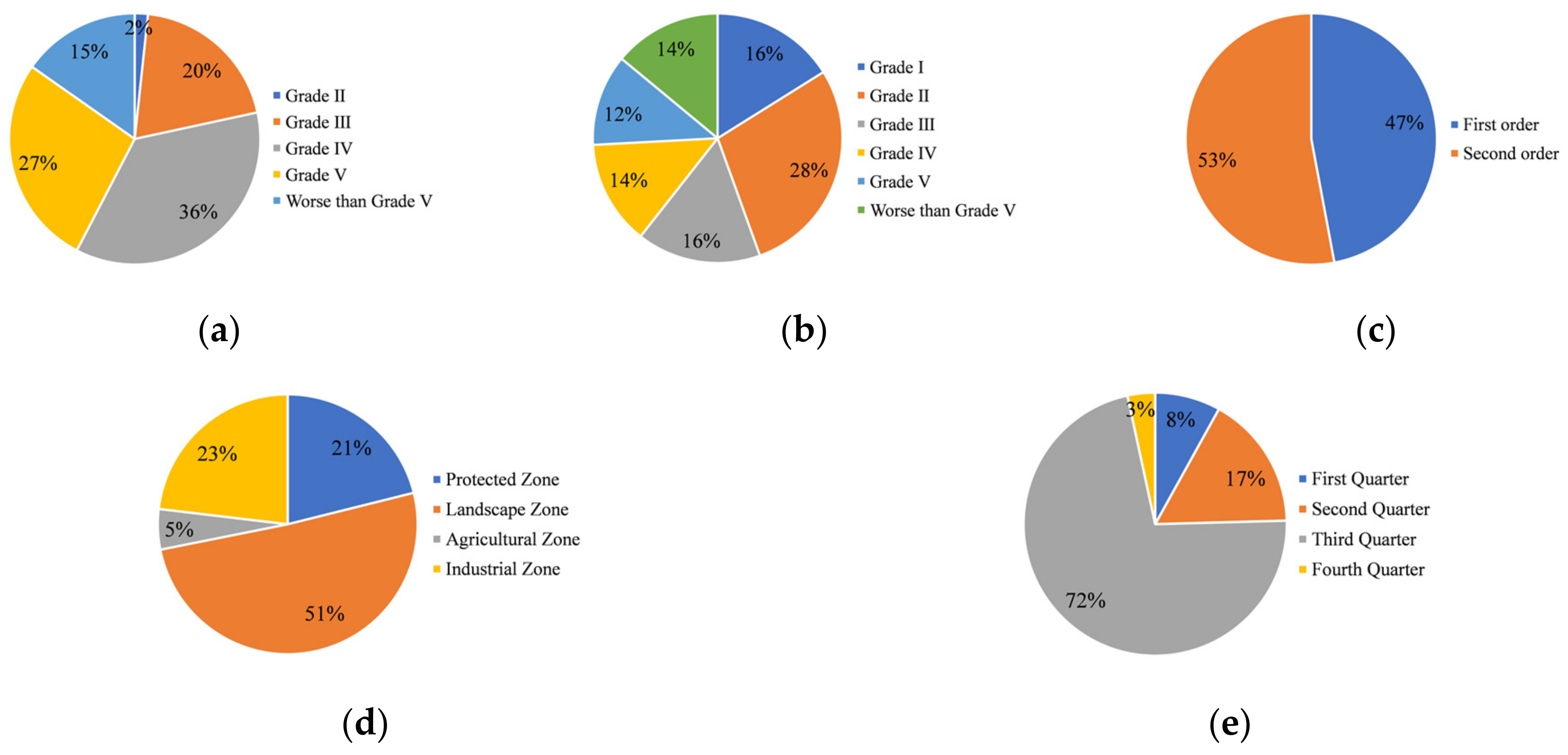
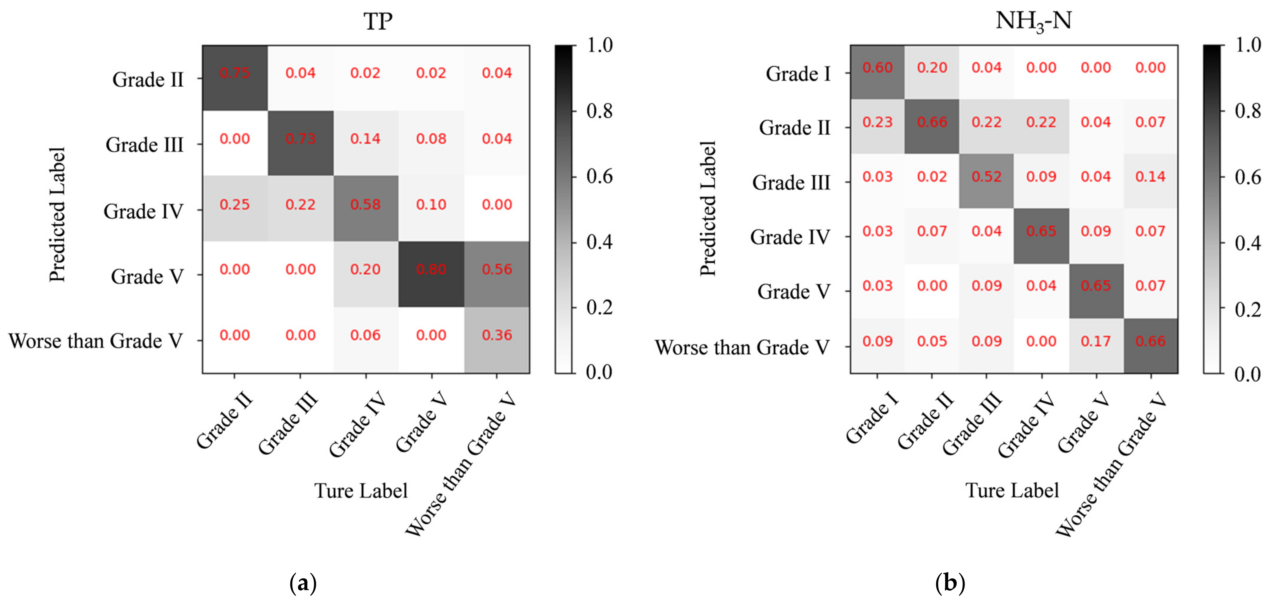
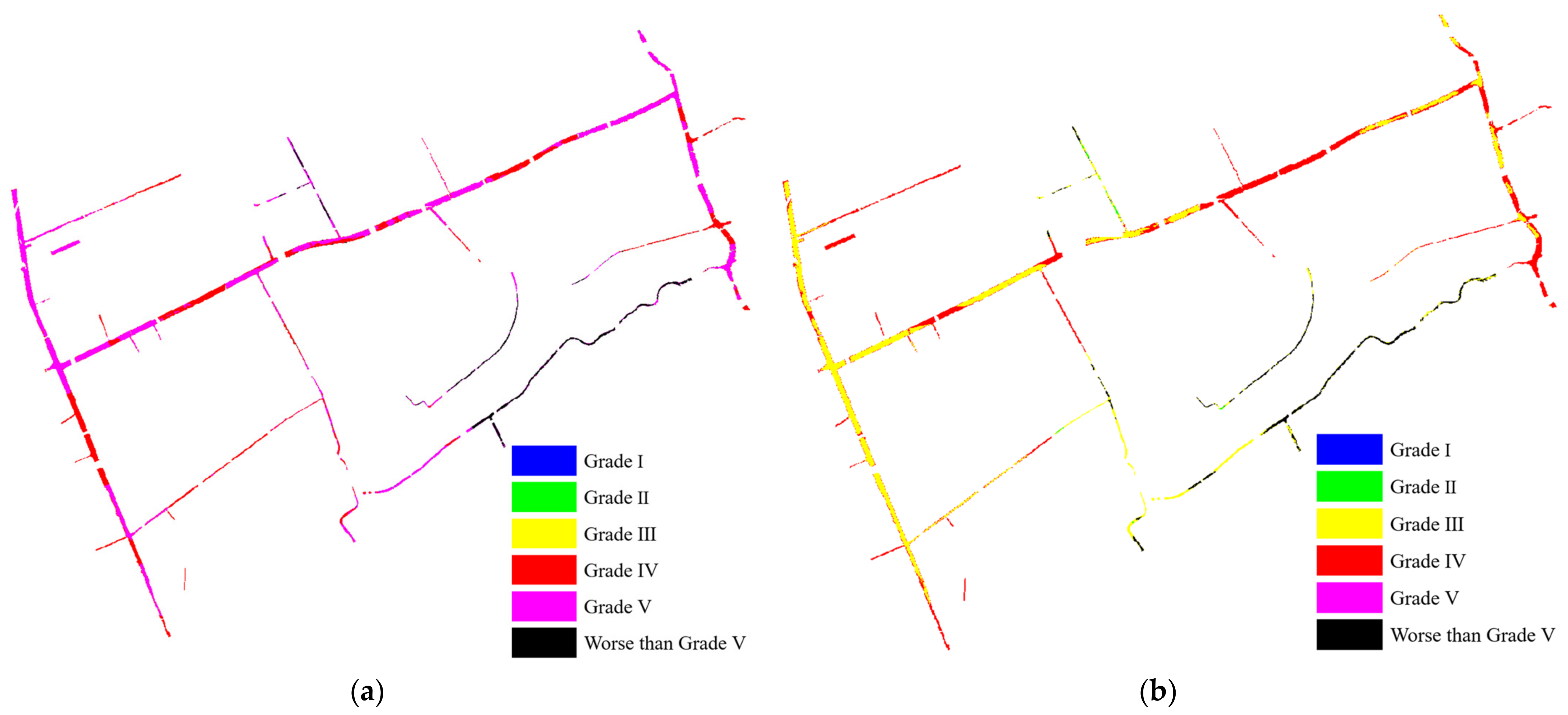
3.3.2. Water Quality Grading Results

With the reflectance map and ensemble learning models, the grading results of TP and NH₃-N were generated. According to the six grades, the grading results were represented by six colors, which are shown in Figure 13.

From the results, the TP situation of Yanghang town was mainly concentrated in grade IV, grade V, and worse than grade V. The second-order rivers, namely Yangsheng River, Meipu River, and Beisitang River, showed a similar water quality situation. Most of the river basins were grade V, and the other parts were grade IV. The TP situation of first-order rivers appeared to be worse than that of second-order rivers. Many river basins were worse than grade V.

The situation of NH₃-N was better than TP, which was mainly concentrated in grade III, grade IV, and worse than grade V. As with the trend of TP, NH₃-N was mainly grade III in Yangsheng River and the river upstream of Meipu River, but was grade IV in the river downstream of Meipu River. Unlike from TP, Beisitang River was between grade III and grade IV. The NH₃-N of the first-order rivers was distributed among grade II, grade III, and worse than grade V.

Compared with the checkpoints, the grading accuracy rates of TP and NH₃-N were both 0.67, respectively. For TP, checkpoints 4, 11, and 13 were overestimated by one grade. Checkpoint 8 was underestimated by one grade. Checkpoint 14 was overestimated by two grades. For NH₃-N, checkpoints 5 and 15 were overestimated by one grade. Checkpoints 6 and 9 were underestimated by one grade. Checkpoint 11 was overestimated by two grades (

Table 4. Difference between the grading result and true grade of each checkpoint.

Checkpoint Number	TP	NH3-N
1	0	0
2	0	0
3	0	0
4	+1	0
5	0	+1
6	0	−1
7	0	0
8	−1	0
9	0	−1
10	0	0
11	+1	+2
12	0	0
13	+1	0
14	+2	0
15	0	+1

). The statistics of the water quality grading accuracy are shown in

Table 5. Statistics of water quality grading precision.

Grading Results	TP	NH3-N
Correct grading	10	10
Overestimate 1 grade	3	2
Underestimate 1 grade	1	2
Overestimate 2 grades	1	1
Grading precision	0.67	0.67

.

4. Discussion

Multispectral remote sensing technology has been applied to monitor water quality for several decades. Researchers have proposed many effective methods to infer the water quality from spectral reflectance values or multispectral images. However, for complex urban river networks, it is still a new application field. In fact, a high-efficiency, high-frequency, and whole-basin water quality monitoring method is an urgent need for urban rivers because of the complexity, diversity, and variability of urban rivers. Aiming to address the practical need, our research proposed a spectral- and spatial-integrated ensemble learning method for urban river network water quality grading. The experiment in this paper proved that our method is an improvement for urban river water quality remote sensing.

4.1. Dataset Construction

In situ data collection is a key step before water quality remote sensing. To construct the water quality parameter inversion models, researchers collected their datasets. Usually, studies have focused on one or several rivers or lakes [46,71,72]. Therefore, the data collection areas were usually among these rivers or lakes. Additionally, water and spectrum sampling are works that require considerable labor power and time. This means that the samples are limited. Furthermore, these datasets mainly include spectrum and water quality data. However, water pollution is affected by many factors, such as the surrounding environment and climate. Remote sensing is a technology that can analyze spatial properties accurately. Thus, it is meaningful and feasible to add spatial property analysis to remote sensing water quality monitoring.

For river networks in large cities, it is almost impossible to cover all rivers and all environmental situations. Thus, collecting representative data is significant to extract the main features for urban water quality remote sensing. In this paper, the water functional zone, stream order, water quality diversity, and seasons were taken into consideration. This is a requirement we proposed for urban water quality remote sensing dataset collection that can be a reference for sampling. In the future, more samples will be added to our dataset. Furthermore, other environmental features will be considered. For example, the recent precipitation affects the discharge, which can directly worsen the water quality. Other features, such as the distribution of discharge outlets and isolation fences in the river, also affect the water quality. Thus, the dataset can be expanded and more reasonable.

4.2. Feature Analysis

Spectral feature analysis is an important step for remote sensing that aims to establish a connection between spectrum and observation targets. To avoid band redundancy, we chose to select feature bands in advance and use a multispectral camera. The band-selection methods usually only consider the spectrum feature. For environmental observations, it is also important to analyze the correlation between bands and the target. For multispectral cameras, bandwidth is another problem that needs to be considered, because bandwidth can affect the observation accuracy and image quality. Based on the aims and problems above, a feature analysis process was proposed. The features selected in this paper are proven effective according to the modeling and application experiment results. This analysis method also has some areas to improve in the future. Other methods, such as dimensionality reduction [13], clustering [14], and ranking [15], can be used to select the center wavelength, which may extract more potential bands. Other indexes can also be used to calculate the best bandwidth range. For example, camera performance is another aspect that can be considered.

Spatial features are a new and significant type of feature used in the model for remote sensing water quality monitoring in this paper. The water’s functional zone [21] and hydrodynamics [23] are two key factors that affect the water’s quality. We proved that the spatial features improve the grading accuracy. Furthermore, despite these two factors, other spatial factors or even environmental factors may also affect water quality, such as climate. Thus, which spatial or environmental features are the main features that can affect the inversion model is a topic worth studying.

4.3. Water Quality Grading Model

Water quality inversion modeling is the most important and difficult step in water quality remote sensing. TP and NH₃-N are two of the most significant water pollutants that need to be monitored. In future studies, the models for grading other water quality parameters will also be established. In this paper, to meet the actual needs of municipal water affairs, a model was established to grade TP and NH₃-N. Three strategies were used to improve the grading accuracy: adding spatial features, using ensemble learning, and using hard-soft fused voting. From the five-fold cross validation results, it can be clearly seen that these three strategies can improve the accuracy and generalization ability. Compared to the traditional machine-learning models using only spectral features, the macro precision, macro recall, and macro F1 scores improved from approximately 0.30 to approximately 0.60 when using our model. However, the evaluation indexes of the model show that the model can still be improved. We hope the accuracy can be improved to 0.80. By introducing the concentration of optically relevant components and other features that affect the water quality, the model can have a higher interpretability and accuracy. The inversion model can be improved using better machine-learning methods and voting methods. There are also limitations to this model. The machine-learning method itself also has weaknesses. If water quality measurement errors occur before establishing the model, this can have big consequences. Therefore, improving the robustness of the model is significant. In addition, not all regions have a strictly divided water functional zone. The spatial features used in the model need further improvement.

4.4. Application Process

To date, many researchers have performed numerous experiments with images collected with UAVs [42], aircraft [73], or satellites [74,75]. We hope to make remote sensing a routine monitoring method to support traditional water quality monitoring methods. Aiming to achieve this goal, we proposed a complete a feasible application process. The results prove that this process can be used for UAV-borne remote sensing water quality monitoring. Based on this process, some improvements can be made. For the data collection step, the flight route can be more targeted. For example, a long strip river may use a patrol route. The image correction method followed the calibration and correction method of the satellite multispectral camera. However, low-altitude remote sensing may require a more appropriate sensor-calibration and image-correction method. The water part image extraction step can use machine-learning to clip the image automatically. Furthermore, because of the object shadows on the shore, the grading results of some river parts appear to be a grade jump. How to deal with shadows is also a problem that needs to be considered. Thus, more work needs to be done in the future to achieve routine monitoring using remote sensing technology.

5. Conclusions

Whole-basin and high-frequency monitoring is an urgent need for urban river network water quality monitoring. Remote sensing is an appropriate technology to address this problem. Aiming to accurately invert the water quality situation, it is necessary to extract suitable features and establish a more universal model for key water quality parameters.

We proposed a spectral- and spatial-integrated ensemble learning method for urban river network water quality grading. The method includes three parts: an in situ sampling method and a practical application process, a feature analysis process, and spectral- and spatial-feature integrated water quality grading modeling. The sampling method aims to provide a reference to handle the problem of numerous rivers and complex environmental influences. Based on the sampling condition requirements, a representative dataset for urban water quality remote sensing can be collected. For multispectral cameras used for water quality remote sensing, we provide a process to select the bands, which also includes bandwidth analysis. Spatial features are the new features that were added in our study. The spatial features proved that they can improve the water quality grading accuracy. An ensemble learning model with a hard-soft fused voting method was proposed by using both spectral and spatial features. The new model can improve the TP and NH₃-N grading macro precision, macro recall, and macro F1 scores from approximately 0.30 to approximately 0.60, compared to the traditional machine-learning models, using only spectral features. Finally, an application process was proposed that was proven feasible. The precision of both the TP and NH₃-N grading results was 0.67.

The method proposed in this paper can extract suitable features and build a relationship model between the features and water quality. This model improves the accuracy of the water quality inversion model for complex urban river networks, which means it is more universal than other existing models. Based on UAV-borne multispectral remote sensing technology, our method can effectively deal with the high-efficiency, high-frequency, and whole-basin water quality monitoring problem. However, as also recommended in the discussion, further studies are needed to improve the grading result’s accuracy. In the future, we hope to make remote sensing a routine monitoring method to support traditional water quality monitoring methods.

References

1. Wang, Y.; Xian, C.; Jiang, Y.; Pan, X.; Ouyang, Z. Anthropogenic reactive nitrogen releases and gray water footprints in urban water pollution evaluation: The case of Shenzhen City, China. Environ. Dev. Sustain. 2019, 22, 6343–6361. [Google Scholar] [CrossRef]
2. Ye, Q. Quality evaluation of ecological restoration of urban water pollution based on analytic hierarchy process. J. Coastal Res. 2020, 104, 10–13. [Google Scholar] [CrossRef]
3. Huang, B.C.; He, C.S.; Fan, N.S.; Jin, R.C.; Yu, H. Envisaging wastewater-to-energy practices for sustainable urban water pollution control: Current achievements and future prospects. Renew. Sustain. Energy Rev. 2020, 134, 110134. [Google Scholar] [CrossRef]
4. Qu, M.; Lefebvre, D.D.; Wang, Y.; Qu, Y.; Zhu, D.; Ren, W. Algal blooms: Proactive strategy. Science 2014, 346, 175–176. [Google Scholar] [CrossRef] [PubMed]
5. Zhang, W.; Jin, X.; Liu, D.; Lang, C.; Shan, B. Temporal and spatial variation of nitrogen and phosphorus and eutrophication assessment for a typical arid river—Fuyang River in northern China. J. Environ. Sci. 2017, 55, 41–48. [Google Scholar] [CrossRef]
6. Gobler, C.; Burkholder, J.; Davis, T.; Harke, M.J.; Johengen, T.; Stow, C.; Waal, D.B.V.d. The dual role of nitrogen supply in controlling the growth and toxicity of cyanobacterial blooms. Harmful Algae 2016, 54, 87–97. [Google Scholar] [PubMed]
7. Niroumand-Jadidi, M.; Bovolo, F.; Bruzzone, L. Novel spectra-derived features for empirical retrieval of water quality parameters: Demonstrations for OLI, MSI, and OLCI sensors. IEEE Trans. Geosci. Remote Sens. 2019, 57, 10285–10300. [Google Scholar] [CrossRef]
8. Wang, X.; Yang, W. Water quality monitoring and evaluation using remote sensing techniques in China: A systematic review. Ecosyst. Health Sustain. 2019, 5, 47–56. [Google Scholar] [CrossRef] [Green Version]
9. Sagan, V.; Peterson, K.T.; Maimaitijiang, M.; Sidike, P.; Sloan, J.; Greeling, B.A.; Maalouf, S.; Adams, C. Monitoring inland water quality using remote sensing: Potential and limitations of spectral indices, bio-optical simulations, machine learning, and cloud computing. Earth-Sci. Rev. 2020, 205. [Google Scholar] [CrossRef]
10. Song, K.; Liu, G.; Wang, Q.; Wen, Z.; Lyu, L.; Du, Y.; Sha, L.; Fang, C. Quantification of lake clarity in China using Landsat OLI imagery data. Remote Sens. Environ. 2020, 243, 111800. [Google Scholar]
11. Gholizadeh, M.H.; Melesse, A.M.; Reddi, L. A comprehensive review on water quality parameters estimation using remote sensing techniques. Sensors 2016, 16, 1298. [Google Scholar] [CrossRef] [PubMed] [Green Version]
12. Spyrakos, E.; O’Donnell, R.; Hunter, P.D.; Miller, C.; Scott, M.; Simis, S.G.H.; Neil, C.; Barbosa, C.C.F.; Binding, C.E.; Bradt, S.; et al. Optical types of inland and coastal waters. Limnol. Oceanogr. 2018, 63, 846–870. [Google Scholar] [CrossRef] [Green Version]
13. Long, Y.; Rivard, B.; Rogge, D.; Tian, M. Hyperspectral band selection using the N-dimensional Spectral Solid Angle method for the improved discrimination of spectrally similar targets. Int. J. Appl. Earth Obs. Geoinf. 2019, 79, 35–47. [Google Scholar]
14. Wang, Q.; Zhang, F.; Li, X. Optimal clustering framework for hyperspectral band selection. IEEE Trans. Geosci. Remote Sens. 2018, 56, 5910–5922. [Google Scholar] [CrossRef] [Green Version]
15. Jia, S.; Tang, G.; Zhu, J.; Li, Q. A novel ranking-based clustering approach for hyperspectral band selection. IEEE Trans. Geosci. Remote Sens. 2016, 54, 88–102. [Google Scholar] [CrossRef]
16. Yan, F.; Wang, S.; Zhou, Y.; Zhao, Q.; Zhou, W.; Zhu, L.; Du, X.; Chen, S.; Wang, L.; Zhang, P. Correlation analysis of spectral reflectance in determining preliminary algorithms for water quality monitoring in Taihu Lake, China. In Proceedings of the IGARSS 2004, IEEE International Geoscience and Remote Sensing Symposium, Anchorage, AK, USA, 20–24 September 2004; Volume 7, pp. 4889–4892. [Google Scholar]
17. Lee, Z.; Weidemann, A.; Arnone, R. Combined effect of reduced band number and increased bandwidth on shallow water remote sensing: The case of WorldView 2. IEEE Trans. Geosci. Remote Sens. 2013, 51, 2577–2586. [Google Scholar] [CrossRef]
18. Cao, Z.; Ma, R.; Duan, H.; Xue, K. Effects of broad bandwidth on the remote sensing of inland waters: Implications for high spatial resolution satellite data applications. ISPRS J. Photogramm. Remote Sens. 2019, 153, 110–122. [Google Scholar] [CrossRef]
19. Liu, C.; Zeng, D.; Wu, H.; Wang, Y.; Jia, S.; Xin, L. Urban land cover classification of high-resolution aerial imagery using a relation-enhanced multiscale convolutional network. Remote Sens. 2020, 12, 311. [Google Scholar] [CrossRef] [Green Version]
20. He, X.; Li, P. Surface water pollution in the middle chinese loess plateau with special focus on hexavalent chromium (Cr6+): Occurrence, sources and health risks. Expo. Health 2020, 12, 385–401. [Google Scholar] [CrossRef]
21. Ping, G.; Ya-Shan, S.; Chao, Y. Water function zoning and water environment capacity analysis on surface water in Jiamusi urban area. Procedia Eng. 2012, 28, 458–463. [Google Scholar] [CrossRef] [Green Version]
22. Rong, W.; Tian-Yin, H.; Wei, W. Different factors on nitrogen and phosphorus self-purification ability from an urban Guandu-Huayuan river. J. Lake Sci. 2016, 28, 105–113. [Google Scholar] [CrossRef] [Green Version]
23. Zhou, H.; Chen, X.; Ying, T.; Xuan, Y.; Wangjin, Y.; Liu, X. Variations and behavior of wastewater-marking pharmaceuticals influenced under hydrodynamic conditions in urban river systems. Int. J. Environ. Sci. Technol. 2018, 16, 5669–5684. [Google Scholar] [CrossRef]
24. Wu, C.; Wu, J.; Qi, J.; Zhang, L.; Huang, H.; Lou, L.; Chen, Y. Empirical estimation of total phosphorus concentration in the mainstream of the Qiantang River in China using Landsat TM data. Int. J. Remote Sens. 2010, 31, 2309–2324. [Google Scholar] [CrossRef]
25. Du, C.; Wang, Q.; Li, Y.; Lyu, H.; Zhu, L.; Zheng, Z.; Wen, S.; Liu, G.; Guo, Y. Estimation of total phosphorus concentration using a water classification method in inland water. Int. J. Appl. Earth Obs. Geoinf. 2018, 71, 29–42. [Google Scholar] [CrossRef]
26. Ogashawara, I.; Li, L. Removal of Chlorophyll-a Spectral Interference for Improved Phycocyanin Estimation from Remote Sensing Reflectance. Remote Sens. 2019, 11, 1764. [Google Scholar] [CrossRef] [Green Version]
27. Liu, G.; Li, S.; Song, K.; Wang, X.; Wen, Z.; Kutser, T.; Jacinthe, P.-A.; Shang, Y.; Lyu, L.; Fang, C.; et al. Remote sensing of CDOM and DOC in alpine lakes across the Qinghai-Tibet Plateau using Sentinel-2A imagery data. J. Environ. Manag. 2021, 286, 112231. [Google Scholar] [CrossRef]
28. Giardino, C.; Candiani, G.; Bresciani, M.; Lee, Z.; Gagliano, S.; Pepe, M. BOMBER: A tool for estimating water quality and bottom properties from remote sensing images. Comput. Geosci. 2012, 45, 313–318. [Google Scholar] [CrossRef]
29. Albert, A.; Gege, P. Inversion of irradiance and remote sensing reflectance in shallow water between 400 and 800 nm for calculations of water and bottom properties. Appl. Opt. 2006, 45, 2331–2343. [Google Scholar] [CrossRef]
30. Chang, N.; Imen, S.; Vannah, B. Remote sensing for monitoring surface water quality status and ecosystem state in relation to the nutrient cycle: A 40-year perspective. Crit. Rev. Environ. Sci. Technol. 2015, 45, 101–166. [Google Scholar] [CrossRef]
31. Kutser, T.; Herlevi, A.; Kallio, K.; Arst, H. A hyperspectral model for interpretation of passive optical remote sensing data from turbid lakes. Sci. Total Environ. 2001, 268, 47–58. [Google Scholar] [CrossRef]
32. Wang, P.; Boss, E.; Roesler, C. Uncertainties of inherent optical properties obtained from semianalytical inversions of ocean color. Appl. Opt. 2005, 44, 4074–4085. [Google Scholar] [CrossRef] [PubMed]
33. Tung, T.M.; Yaseen, Z.M. A survey on river water quality modelling using artificial intelligence models: 2000–2020. J. Hydrol. 2020, 585, 124670. [Google Scholar] [CrossRef]
34. Wang, X.; Zhang, F.; Ding, J. Evaluation of water quality based on a machine learning algorithm and water quality index for the Ebinur Lake Watershed, China. Sci. Rep. 2017, 7, 12858. [Google Scholar] [CrossRef] [Green Version]
35. Maier, P.; Keller, S. Machine Learning Regression on Hyperspectral Data to Estimate Multiple Water Parameters. In Proceedings of the 2018 9th Workshop on Hyperspectral Image and Signal Processing: Evolution in Remote Sensing (WHISPERS), Amsterdam, The Netherlands, 23–26 September 2018; pp. 1–5. [Google Scholar]
36. Wang, X.; Ma, L. Apply semi-supervised support vector regression for remote sensing water quality retrieving. In Proceedings of the 2010 IEEE International Geoscience and Remote Sensing Symposium, Honolulu, HI, USA, 25–30 July 2010; pp. 2757–2760. [Google Scholar]
37. Zhang, Y.; Wu, L.; Ren, H.; Liu, Y.; Zheng, Y.; Liu, Y.; Dong, J. Mapping water quality parameters in urban rivers from hyperspectral images using a new self-adapting selection of multiple artificial neural networks. Remote Sens. 2020, 12, 336. [Google Scholar] [CrossRef] [Green Version]
38. Peterson, K.; Sagan, V.; Sidike, P.; Cox, A.L.; Martinez, M. Suspended Sediment Concentration Estimation from Landsat Imagery along the Lower Missouri and Middle Mississippi Rivers Using an Extreme Learning Machine. Remote Sens. 2018, 10, 1503. [Google Scholar] [CrossRef] [Green Version]
39. Peterson, K.; Sagan, V.; Sloan, J. Deep learning-based water quality estimation and anomaly detection using Landsat-8/Sentinel-2 virtual constellation and cloud computing. GIScience Remote Sens. 2020, 57, 510–525. [Google Scholar]
40. Dong, X.; Yu, Z.; Cao, W.; Shi, Y.; Ma, Q. A survey on ensemble learning. Front. Comput. Sci. 2019, 14, 241–258. [Google Scholar] [CrossRef]
41. Peterson, K.T.; Sagan, V.; Sidike, P.; Hasenmueller, E.A.; Sloan, J.J.; Knouft, J.H. Machine learning-based ensemble prediction of water-quality variables using feature-level and decision-level fusion with proximal remote sensing. Photogramm. Eng. Remote Sens. 2019, 85, 269–280. [Google Scholar] [CrossRef]
42. Stöcker, C.; Bennett, R.; Nex, F.; Gerke, M.; Zevenbergen, J. Review of the current state of UAV regulations. Remote Sens. 2017, 9, 459. [Google Scholar] [CrossRef] [Green Version]
43. Liu, C.; Zhou, X.; Zhou, Y.; Akbar, A. Multi-temporal monitoring of urban river water quality using UAV-Borne multi-spectral remote sensing. Int. Arch. Photogramm. Remote Sens. Spatial Inf. Sci. 2020, XLIII-B3-2020, 1469–1475. [Google Scholar] [CrossRef]
44. McEliece, R.; Hinz, S.; Guarini, J.M.; Coston-Guarini, J. Evaluation of nearshore and offshore water quality assessment using UAV multispectral imagery. Remote Sens. 2020, 12, 2258. [Google Scholar] [CrossRef]
45. Su, T.-C. A study of a matching pixel by pixel (MPP) algorithm to establish an empirical model of water quality mapping, as based on unmanned aerial vehicle (UAV) images. Int. J. Appl. Earth Obs. Geoinf. 2017, 58, 213–224. [Google Scholar] [CrossRef]
46. Wei, L.; Huang, C.; Wang, Z.; Wang, Z.; Zhou, X.; Cao, L. Monitoring of urban black-odor water based on nemerow index and gradient boosting decision tree regression using UAV-Borne hyperspectral imagery. Remote Sens. 2019, 11, 2402. [Google Scholar] [CrossRef] [Green Version]
47. Ouillon, S.; Petrenko, A. Above-water measurements of reflectance and chlorophyll-a algorithms in the Gulf of Lions, NW Mediterranean Sea. Opt. Express 2005, 13, 2531–2548. [Google Scholar] [CrossRef] [PubMed]
48. Mueller, J.L.; Fargion, G.; McClain, C.; Mueller, J.; Frouin, R.; Davis, C.; Arnone, R.; Carder, K.; Mobley, C.; McLean, S.; et al. Ocean Optics Protocols for Satellite Ocean Color Sensor Validation, Revision 4. Volume III: Radiometric Measurements and Data Analysis Protocols; National Aeronautical and Space Administration: Greenbelt, MD, USA, 2003. [Google Scholar]
49. The Ministry of Environmental Protection of the People’s Republic of China. Environmental Quality Standards for Surface Water (GB 3838–2002); The Ministry of Environmental Protection of the People’s Republic of China: Beijing, China, 2002. [Google Scholar]
50. Shanghai Water Authority. Functional Zoning of Water Environment in Shanghai; Shanghai Water Authority: Shanghai, China, 2004. [Google Scholar]
51. Scheidegger, A.E. Horton’s law of stream numbers. Water Resour. Res. 1968, 4, 655–658. [Google Scholar] [CrossRef]
52. Ma, X.; Wang, L.; Yang, H.; Li, N.; Gong, C. Spatiotemporal Analysis of Water Quality Using Multivariate Statistical Techniques and the Water Quality Identification Index for the Qinhuai River Basin, East China. Water 2020, 12, 2764. [Google Scholar] [CrossRef]
53. Wang, J.; Fu, Z.; Qiao, H.; Liu, F. Assessment of eutrophication and water quality in the estuarine area of Lake Wuli, Lake Taihu, China. Sci. Total Environ. 2019, 650 Pt 1, 1392–1402. [Google Scholar] [CrossRef] [PubMed]
54. Wang, M. Effects of ocean surface reflectance variation with solar elevation on normalized water-leaving radiance. Appl. Opt. 2006, 45, 4122–4128. [Google Scholar] [CrossRef]
55. Schramm, S.; Rangel, J.; Salazar, D.A.; Schmoll, R.; Kroll, A. Target analysis for the multispectral geometric calibration of cameras in visual and infrared spectral range. IEEE Sens. J. 2021, 21, 2159–2168. [Google Scholar] [CrossRef]
56. Oniga, V.E.; Pfeifer, N.; Loghin, A.M. 3D calibration test-field for digital cameras mounted on unmanned aerial systems (UAS). Remote Sens. 2018, 10, 2017. [Google Scholar] [CrossRef] [Green Version]
57. Jiang, Y.H.; Zhang, G.; Tang, X.; Li, D.; Huang, W.; Pan, H.B. Geometric calibration and accuracy assessment of ZiYuan-3 multispectral images. IEEE Trans. Geosci. Remote Sens. 2014, 52, 4161–4172. [Google Scholar] [CrossRef]
58. Cao, S.; Danielson, B.; Clare, S.; Koenig, S.; Campos-Vargas, C.; Sanchez-Azofeifa, A. Radiometric calibration assessments for UAS-borne multispectral cameras: Laboratory and field protocols. ISPRS J. Photogramm. Remote Sens. 2019, 149, 132–145. [Google Scholar] [CrossRef]
59. Kelcey, J.; Lucieer, A. Sensor correction of a 6-band multispectral imaging sensor for UAV remote sensing. Remote Sens. 2012, 4, 1462–1493. [Google Scholar] [CrossRef] [Green Version]
60. Dinguirard, M.; Slater, P.N. Calibration of space-multispectral imaging sensors. Remote Sens. Environ. 1999, 68, 194–205. [Google Scholar] [CrossRef]
61. Sekrecka, A.; Wierzbicki, D.; Kedzierski, M. Influence of the sun position and platform orientation on the quality of imagery obtained from unmanned aerial vehicles. Remote Sens. 2020, 12, 1040. [Google Scholar] [CrossRef] [Green Version]
62. Minařík, R.; Langhammer, J.; Hanuš, J. Radiometric and atmospheric corrections of multispectral μMCA camera for UAV spectroscopy. Remote Sens. 2019, 11, 2428. [Google Scholar] [CrossRef] [Green Version]
63. Del Pozo, S.; Rodríguez-Gonzálvez, P.; Hernández-López, D.; Felipe-García, B. Vicarious radiometric calibration of a multispectral camera on board an unmanned aerial system. Remote Sens. 2014, 6, 1918–1937. [Google Scholar] [CrossRef] [Green Version]
64. Woods, C.M.; Edwards, M.C. 12 factor analysis and related methods. In Epidemiology and Medical Statistics; Rao, C.R., Miller, J.P., Rao, D.C., Eds.; Handbook of Statistics; Elsevier: Amsterdam, The Netherlands, 2007; pp. 367–394. [Google Scholar]
65. Koo, T.K.; Li, M.Y. A guideline of selecting and reporting intraclass correlation coefficients for reliability research. J. Chiropr. Med. 2016, 15, 155–163. [Google Scholar] [CrossRef] [Green Version]
66. Akaho, S. A kernel method for canonical correlation analysis. arXiv 2006, arXiv:cs/0609071. [Google Scholar]
67. Chen, T.; Guestrin, C. XGBoost: A scalable tree boosting system. In Proceedings of the 22nd ACM SIGKDD International Conference on Knowledge Discovery and Data Mining, New York, NY, USA, 13–17 August 2016; pp. 785–794. [Google Scholar]
68. Cheng, S.; Zhang, S.; Li, L.; Zhang, D. Water quality monitoring method based on TLD 3D fish tracking and XGBoost. Math. Probl. Eng. 2018, 2018, 1–12. [Google Scholar] [CrossRef] [Green Version]
69. Leitner, F.; Mardis, S.A.; Krallinger, M.; Cesareni, G.; Hirschman, L.; Valencia, A. An Overview of BioCreative II.5. IEEE/ACM Trans. Comput. Biol. Bioinform. 2010, 7, 385–399. [Google Scholar] [CrossRef] [Green Version]
70. Wang, X.; Chen, S.; Su, J. Real Network Traffic Collection and Deep Learning for Mobile App Identification. Wirel. Commun. Mob. Comput. 2020, 2020, 4707909:4707901–4707909:4707914. [Google Scholar] [CrossRef]
71. Morgan, B.J.; Stocker, M.D.; Valdes-Abellan, J.; Kim, M.S.; Pachepsky, Y. Drone-based imaging to assess the microbial water quality in an irrigation pond: A pilot study. Sci. Total Environ. 2020, 716, 135757. [Google Scholar] [CrossRef]
72. Keith, D.J.; Schaeffer, B.A.; Lunetta, R.S.; Gould, R.W.; Rocha, K.; Cobb, D.J. Remote sensing of selected water-quality indicators with the hyperspectral imager for the coastal ocean (HICO) sensor. Int. J. Remote Sens. 2014, 35, 2927–2962. [Google Scholar] [CrossRef]
73. Olmanson, L.G.; Brezonik, P.L.; Bauer, M.E. Airborne hyperspectral remote sensing to assess spatial distribution of water quality characteristics in large rivers: The Mississippi River and its tributaries in Minnesota. Remote Sens. Environ. 2013, 130, 254–265. [Google Scholar] [CrossRef]
74. Urbanski, J.A.; Wochna, A.; Bubak, I.; Grzybowski, W.; Lukawska-Matuszewska, K.; Łącka, M.; Śliwińska, S.; Wojtasiewicz, B.; Zajączkowski, M. Application of Landsat 8 imagery to regional-scale assessment of lake water quality. Int. J. Appl. Earth Obs. Geoinf. 2016, 51, 28–36. [Google Scholar] [CrossRef]
75. Liu, D.; Yu, S.; Cao, Z.; Qi, T.; Duan, H. Process-oriented estimation of column-integrated algal biomass in eutrophic lakes by MODIS/Aqua. Int. J. Appl. Earth Obs. Geoinf. 2021, 99, 102321. [Google Scholar] [CrossRef]
Figure 1. Sampling area and the sampling point location (I: Jinhuigang River, Punan Canal, and Qingcun Twon, Fengxian District. II: Yanghang Town, Baoshan District. III: Chongming District. IV: Taopu River, Baoshan District).
Remotesensing 13 04591 g001
Figure 2. The proportion of different requirements in the dataset. (a) Water quality grades of TP. (b) Water quality grades of NH3-N. (c) Stream order. (d) Water functional zone. (e) Quarter of the year.
Remotesensing 13 04591 g002
Figure 3. Flight zoning, river condition, and checkpoints in the Yanghang Town, Baoshan District, Shanghai study area.
Remotesensing 13 04591 g003
Figure 4. Spectral- and spatial-feature-integrated ensemble learning model for urban water quality grading.
Remotesensing 13 04591 g004
Figure 5. Scree plot for choosing the factor number of factor analysis.
Remotesensing 13 04591 g005
Figure 6. Normalized component results of factor analysis and selected factor ranges for feature bands selection.
Remotesensing 13 04591 g006
Figure 7. Correlation coefficient between spectrum band ratio and water quality parameters of the sampling dataset. (a) TP; (b) NH3-N.
Remotesensing 13 04591 g007
Figure 8. Normalized correlation coefficient between spectrum band ratio and water quality parameters of the sampling dataset. (a) TP; (b) NH3-N.
Remotesensing 13 04591 g008
Figure 9. Selected band ranges of factor analysis, correlation with TP, correlation with NH3-N, and high-priority selected bands.
Remotesensing 13 04591 g009
Figure 10. APD between reflectance of selected center wavelength (675, 705, and 850 nm) and reflectance of different bandwidth. Maximum allowed bandwidth ranges of selected center wavelength.
Remotesensing 13 04591 g010
Figure 11. Macro precision, macro recall, and macro F1 scores of 5-fold validation results and overall results (Case α1: SVM with spectral features. Case α2: MLP with spectral feature. Case α3: XGBoost with spectral features. Case α4: Ensemble learning with spectral features. Case β1: SVM with spectral and spatial features. Case β2: MLP with spectral and spatial features. Case β3: XGBoost with spectral and spatial features. Case β4: Ensemble learning with spectral and spatial features). (ac) TP. (df) NH3-N.
Remotesensing 13 04591 g011
Figure 12. Confusion matrix of water quality grading model using spectral and special features combining the 5-fold results. (a) TP. (b) NH3-N.
Remotesensing 13 04591 g012
Figure 13. Water quality grading result maps. (a) TP. (b) NH3-N.
Remotesensing 13 04591 g013