SAR-Based Flood Monitoring for Flatland with Frequently Fluctuating Water Surfaces: Proposal for the Normalized Backscatter Amplitude Difference Index (NoBADI)

Abstract

Space-based synthetic aperture radar (SAR) is a powerful tool for monitoring flood conditions over large areas without the influence of clouds and daylight. Permanent water surfaces can be excluded by comparing SAR images with pre-flood images, but fluctuating water surfaces, such as those found in flat wetlands, introduce uncertainty into flood mapping results. In order to reduce this uncertainty, a simple method called Normalized Backscatter Amplitude Difference Index (NoBADI) is proposed in this study. The NoBADI is calculated from a post-flood SAR image of backscatter amplitude and multiple images on non-flooding conditions. Preliminary analysis conducted in the US state of Florida, which was affected by Hurricane Irma in September 2017, shows that surfaces frequently covered by water (more than 20% of available data) have been successfully excluded by means of C-/L-band SAR (HH, HV, VV, and VH polarizations). Although a simple comparison of pre-flood and post-flood images is greatly affected by the spatial distribution of the water surface in the pre-flood image, the NoBADI method reduces the uncertainty of the reference water surface. This advantage will contribute in making quicker decisions during crisis management.

1. Introduction

Serious flooding events are caused by extreme weather conditions and seasonal tropical cyclones, and it is important for affected societies to respond quickly to disasters based on spatial awareness of the observed flood extent. Space-borne Synthetic Aperture Radar (SAR), a remote sensing technology from space, is an advanced solution for monitoring large-scale flood disasters extensively and quickly that is not hampered by cloud cover. The easiest method for identifying a flood surface is to extract low backscatter pixels, which in this case includes the permanent water surface. To exclude the permanent water surfaces such as rivers and lakes, significant backscatter reduction from a pre-flood SAR image would be extracted as flood-derived water surfaces [1,2,3,4]. Advanced methods analyze phase information based on the interferometric SAR (InSAR) technology. By means of L-band, C-band, and X-band SAR, not only basic experiments but also operational uses for actual crisis responses have been carried out [5,6].

When the spatial distribution of the water surface is not stable, the difference between the pre-flood and post-flood images becomes uncertain. In particular, low-elevation and flat terrains in the tropics tend to form numerous ponds and lakes with fluctuating water bodies due to intensive monsoon precipitation and other seasonal features. In such a case, different results of flood extraction would be obtained according to the acquisition dates of pre-flood images. This uncertainty might cause difficulties in rapid image analysis during an actual operation of crisis response.

One idea for reducing the uncertainty is to quantify the frequency of water extent in each pixel by considering the average and variability during non-flooding periods. Calculations of these statistical values are common in SAR-related studies, and examples include detecting anomaly pixels of the forest [7]. In this study, therefore, we focus on a simple method calculated from the mean and standard deviation values of multiple non-flooding conditions in addition to a post-flood image, which we call the Normalized Backscatter Amplitude Difference Index (NoBADI) in this study. The objective of this study is to evaluate the benefits of NoBADI applied to hurricane-derived flood areas formed around fluctuating water distributions. The obtained results are assessed by optically derived reference maps of water bodies and other SAR-based results, then possibilities and challenges of NoBADI are discussed.

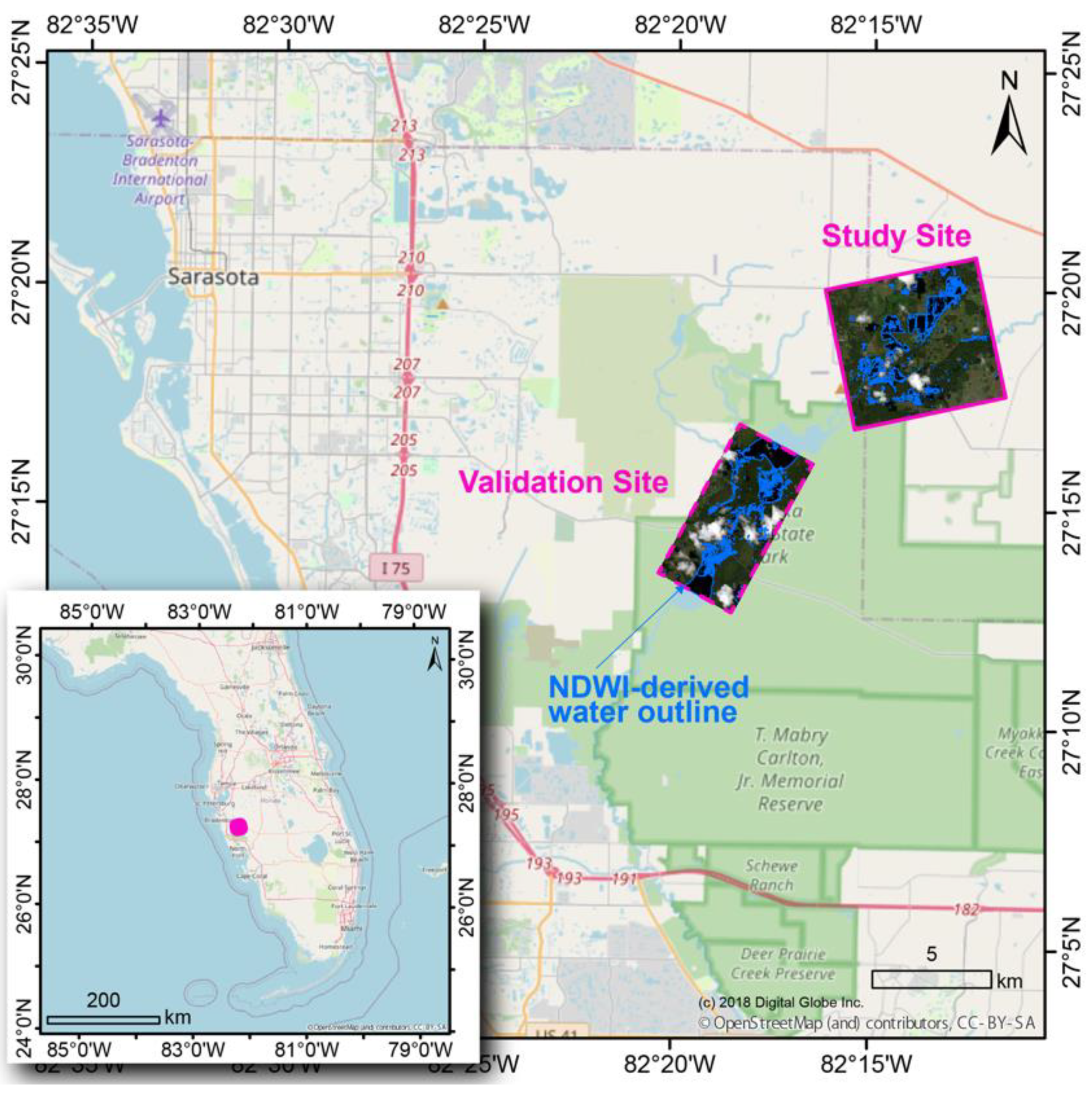
2. Study Site

In this study, we chose the Florida peninsula in the United States as our research site. The study site is rectangular in shape (8.219–8.227° W; 27.281–27.346° N) located 30 km east of Sarasota, upstream of the Myakka River State Park. The site contains the Lettuce Lake (Figure 1). Another rectangle is defined as a validation site in order to assess classification accuracy.

This peninsula is located between the Gulf of Mexico and the Atlantic Ocean. The general climate of the region is characterized by a humid subtropical climate, with rainy seasons from May to October and a dry season from October to the end of April. Average annual precipitation reaches 1137 mm, of which 193 mm is the maximum monthly precipitation in August. Surface temperatures range from 11 to 32 degrees Celsius in Tampa [8].

The topography is dominated by flat terrain and is characterized by the longest coastline in the states of the U.S. (2170 km), where more than half of that is classified as sand beach. Most surfaces in the Florida peninsula have elevations below 5 m. The highest place is the Sugarloaf Mountain (95 m) in the Lake Wales Ridge, located in the center of the peninsula.

The state of Florida, with a population of 19.6 million, was severely damaged by Hurricane Irma. The hurricane formed on the West coast of Africa on 27 August 2017 [9]. It landed in Florida as a Category 4 hurricane on September 10 [10]. Power outages due to the hurricane affected 6.7 million people [11,12], which is equivalent to 36 % of the total population in Florida [12]. Six point five million people were ordered to evacuate and there was a serious problem of traffic congestion [13]. Social disruption caused by the hurricane caused the direct death of 11 people, whereas 115 deaths were indirectly caused by deterioration of the medical environment [14]. The hurricane disappeared and became a tropical storm on 11 September west of Gainesville, Florida [9].

3. Data

3.1. Reference Optical Imagery

Optical satellite imagery collected by WorldView-2 (WV2) derives spatial distribution of post-flood water bodies. The satellite is equipped with a high-resolution optical sensor called the WorldView-110 camera. Satellite operation started in 2009 by DigitalGlobe and is still continued by MAXAR for mostly commercial use and those related to activities for national security. The optical sensor contains eight multispectral bands (coastal, blue, green, yellow, red, red edge, and near-infrared (2)) and one visible panchromatic instrument, with the spatial resolution of 1.85 m and 0.46 m at the nadir angle, respectively [15].

A post-flood WV2 imagery after Hurricane Irma passed was purchased from a Japanese sales agent, Japan Space Imaging. Imagery collection was carried out at 15:59 (UTC), 12 September 2017 under 3% cloud cover condition. The given data consist of a part of multi-spectral bands (blue: 450–510 nm; green 510–580 nm; red 630–690 nm; near-infrared 770–895 nm). Those of product level 2A (standard) after radiometric correction were resampled to 2 m pixel spacing (nearest neighbor) for a WGS84/UTM projection as a 16 bit digital number.

The possible range of water distribution which was not influenced by flood hazards is determined by another optical satellite imagery collected by Sentinel-2 (S2). Identical satellites of Sentinel-2A and Sentinel-2B are operated by the European Space Agency in the Copernicus program to distribute collected data free of charge. The main sensor is a Multi Spectral Instrument (MSI), which contains 12 multispectral bands from coastal to short-wave infrared with the spatial resolutions of 10, 20, and 60 m [16]. Single satellite operations began on 23 June 2015, and dual operations began on 7 March 2017. The revisit period for a single satellite is 10 days. The approximate observation time is 10:30 a.m. local time.

We collected and processed all available S2 data since 27 October 2015 (~325 scenes) in a cloud platform for remote sensing using Google Earth Engine (GEE) (Table S1). These data were observed along the relative orbit number of 97, which was adequate for the study site. Those in product level 2A, surface reflectance at the bottom of atmosphere (after atmospheric correction), were resampled in 10 m (equivalent pixel sizes in a geographic coordination system).

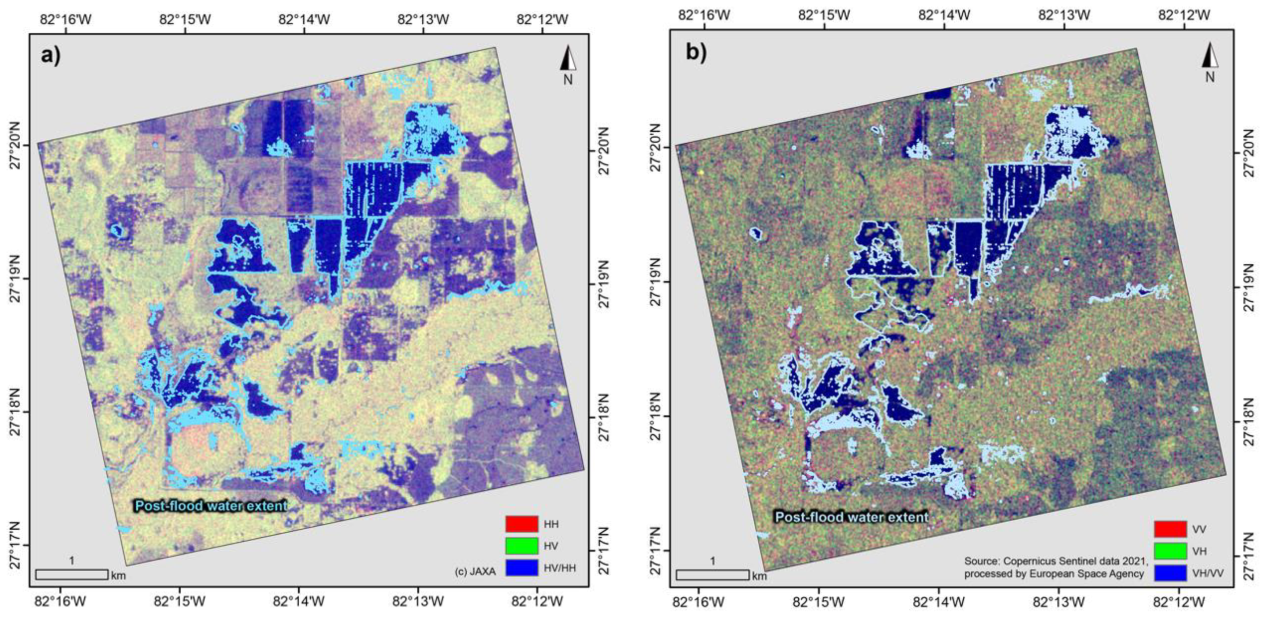
3.2. SAR Data

First, L-band SAR data were collected by the Phased Array type L-band Synthetic Aperture Radar-2 (PALSAR-2) aboard the Advanced Land Observing Satellite-2 (ALOS-2). ALOS-2 was launched on 24 May 2014 and is operated by the Japan Aerospace Exploration Agency (JAXA) for distributing SAR imagery for commercial use or free of charge. Four scenes before the flood (20 January 2015, 1 September 2015, 19 January 2016, and 30 August 2016) and one scene after the flood (12 September 2017) were observed at 5:32 (UTC) from Path 47 (Frame 0530) with an off-nadir angle of 36.6 degrees. Stripmap (fine beam) mode at 5.3/9.1 m spatial resolutions in azimuth/range directions with HH-HV dual polarization (SM3) was selected for these observations.

For the same five scenes, data in two product levels are separately and independently selected for different processes. One is backscatter amplitude image which is ortho-rectified and geocoded by means of SRTM-90 m (v4.1) (i.e., JAXA’s standard product, level 2.1) and resampled (bi-linear) to a pixel spacing of 6.25 m at an adequate WGS84/UTM (zone 17N) projection. Another includes Single Look Complex (SLC) data (i.e., JAXA’s standard product, level 1.1) in which phase information is included for an interferogram. We obtained amplitude (L2.1) data as a 16-bit digital number using the Geotiff format and SLC (L1.1) data in CEOS format.

Second, C-band SAR data were collected by Sentinel-1A/B satellites (S1). These are identical two satellites launched on 3 April 2014 (A) and 25 April 2016 (B) for constellational operation by ESA in the Copernicus program. We collected and processed all available data (~143 scenes) in GEE free of charge (Table S2), which contains data observed on the closest day (15 September 2017) to the flood event (10 September 2017). These data were observed along the relative orbit of 121 (ascending direction) adequate for the study site. ScanSAR (IWS: Interferometric Wide Swath) mode at 20/22m spatial resolutions in azimuth/range directions with VV-VH dual polarization was selected for these S1 observations. The acquired amplitude data were ortho-rectified and resampled to pixel spacing of 10 m (equivalent pixel sizes in a geographic coordination system) as Level-1 Ground Range Detected (GRD) products before our process.

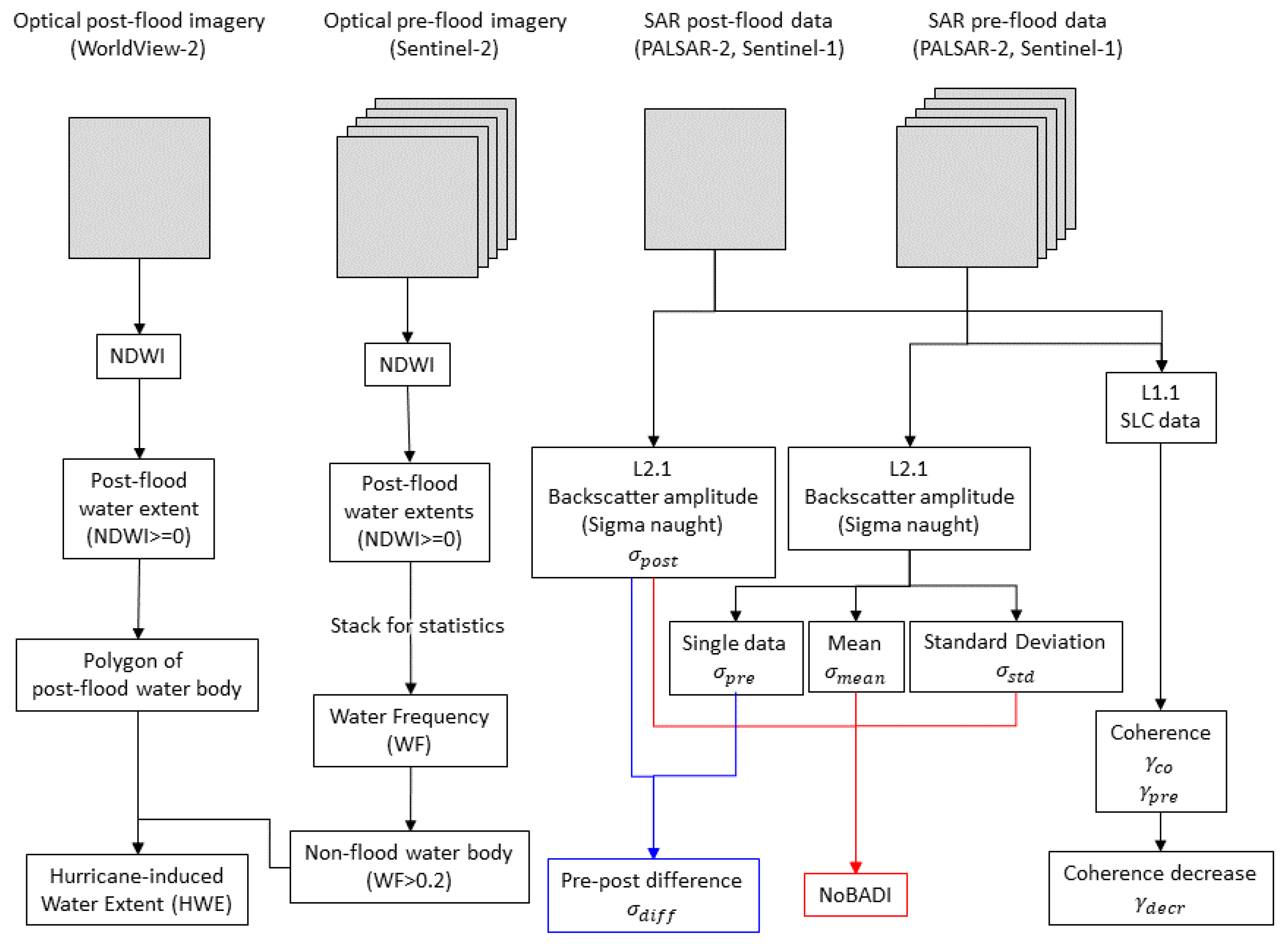
4. Methodology

4.1. Water Surface during the Flood

The post-flood water bodies as references are extracted from the WV2 image (Figure 2). Surface reflectance is calculated from the digital number using conversion parameters explained in [17]. The Normalized Difference Water Index (NDWI) for open water surface proposed by [18] is calculated as follows:

$$\mathrm{NDWI}=\frac{\mathrm{G}-\mathrm{N}}{\mathrm{G}+\mathrm{N}} ,$$

(1)

where G and N are the surface reflectance in the green and near-infrared bands. NDWI is then binarized with a threshold of 0.0, where higher values correspond to the water surface.

4.2. Water Surface Not/Highly Related to the Flood

We generated a water extent map with non-flood status. In the study site, a part of numerous potential water bodies may change their extent due to low-and-flat topography and tropical precipitation. Therefore, only the fixed map of water extent was difficult to determine. Instead, the spatial distribution of the frequency of water cover is quantified in this study. A large number of NDWI images were stacked to quantify water-inundated opportunity at 0 to 100%.

Cloud-covered pixels are excluded with an attached quality band “QA60”. NDWI is then calculated from the green (Band 3) and the near-infrared (Band 8) bands. Binarization of NDWI values with the threshold of 0.0 reclassifies water pixels from other land covers. In each location of the pixels, the number of water pixels divided by total available scene number denotes water frequency (WF). Pixels with permanent water will have a value of 1.0, and pixels with permanent land will have a value of 0.0. WF ranges from 0.0 to 1.0, with larger values for pixels that are covered by water more frequently.

The unique water extent caused by the hurricane Irma (HWE: Hurricane-induced Water Extent) is defined as the difference of WV2-derived water extent and S2-derived frequent water extent with a certain WF value. In the results, HWE is generated based on pre-flood water surface of WF > 0.2.

4.3. L-Band SAR Processing

We calculate NoBADI and other outputs from PALSAR-2 data for flood mapping. As initial processing, backscatter amplitude (i.e., sigma naught) was calculated from the given digital number (DN) in L2.1 data as follows.

$$\mathsf{\sigma }=10{\log }_{10}{\mathrm{DN}}^2-83.$$

(2)

Low-pass filter (mean of 3 × 3 pixels) for speckle noise reduction is conducted, then the pixels are resampled (Nearest Neighbor) relative to the projection of WGS84/UTM (Zone 17N).

This study proposes NoBADI, which expresses how rare the water cover is in each pixel. This value should be intensive/weakened when water covers hardly/frequently inundated places. Non-flood mean value and standard deviation value are calculated from four pre-flood images, which are all of available Stripmap-mode scenes with an equal off-nadir angle in this location. They are combined with post-flood pixel value in order to calculate NoBADI with the following equation:

$$\mathrm{NoBADI}=\frac{{\mathsf{\sigma }}_{\mathrm{post}}-{\mathsf{\sigma }}_{\mathrm{mean}}}{{\mathsf{\sigma }}_{\mathrm{std}}},$$

(3)

where σ_post is the post-flood backscatter amplitude (i.e., sigma naught), σ_mean is the mean of the non-flood backscatter amplitudes, and σ_std is the standard deviation of the non-flood backscatter amplitudes (Figure 2).

The standard deviation shows smaller values for stable land surfaces and larger values for frequently fluctuating surfaces. This method moderates the usual water extent and enhances irregular water extent, even if these have similar values in terms of amplitude decrease over the hurricane-induced flood.

In order to evaluate NoBADI results, general methods of water body extraction are also performed. The simple difference of backscatter amplitude is calculated as follows:

$${\mathsf{\sigma }}_{\mathrm{diff}}={\mathsf{\sigma }}_{\mathrm{post}}-{\mathsf{\sigma }}_{\mathrm{pre}},$$

(4)

where σ_pre is one of four scenes. Four results based on different pre-flood dates are calculated and compared.

In addition, coherence and coherence decreases are calculated by means of SLC (L1.1) data. Interferometric coherence, γ, can be calculated as follows:

$$\mathsf{\gamma }=\frac{\left|\langle {\mathrm{s}}_1{\mathrm{s}}_2^{*}\rangle \right|}{\sqrt{\langle {\mathrm{s}}_1{\mathrm{s}}_1^{*}\rangle \langle {\mathrm{s}}_2{\mathrm{s}}_2^{*}\rangle }},$$

(5)

where s1 and s2 are a pair of single look complex (SLC) SAR data, s* represents the complex conjugate of s, and the bracket 〈 〉 indicates averaging in a local window (4 × 4 pixels in this study). Coherence represents the similarity between two SAR images, and it decreases as the state of the ground surface changes.

To cancel non-hazardous changes from the coherence output, two coherence images including a pre-flood pair (19 January and 30 August 2016), coherence γ_pre, and a pre-flood and post-flood pair (12 September 2017 and 30 August 2016), coherence γ_co, were used. The coherence decrease, γ_decr, is calculated as follows.

$${\mathsf{\gamma }}_{\mathrm{decr}}={\mathsf{\gamma }}_{\mathrm{co}}-{\mathsf{\gamma }}_{\mathrm{pre}}.$$

(6)

4.4. C-Band SAR Processing

Furthermore, we calculated NoBADI from S1 data for flood mapping. Backscatter amplitude (i.e., sigma naught) was ready in GEE. NoBADI is calculated as proposed above, where all available scenes in GEE are stacked in order to calculate the mean and the standard deviation. After the processing, pixels are resampled (Nearest Neighbor) relative to the projection of WGS84/UTM (Zone 17N).

5. Results

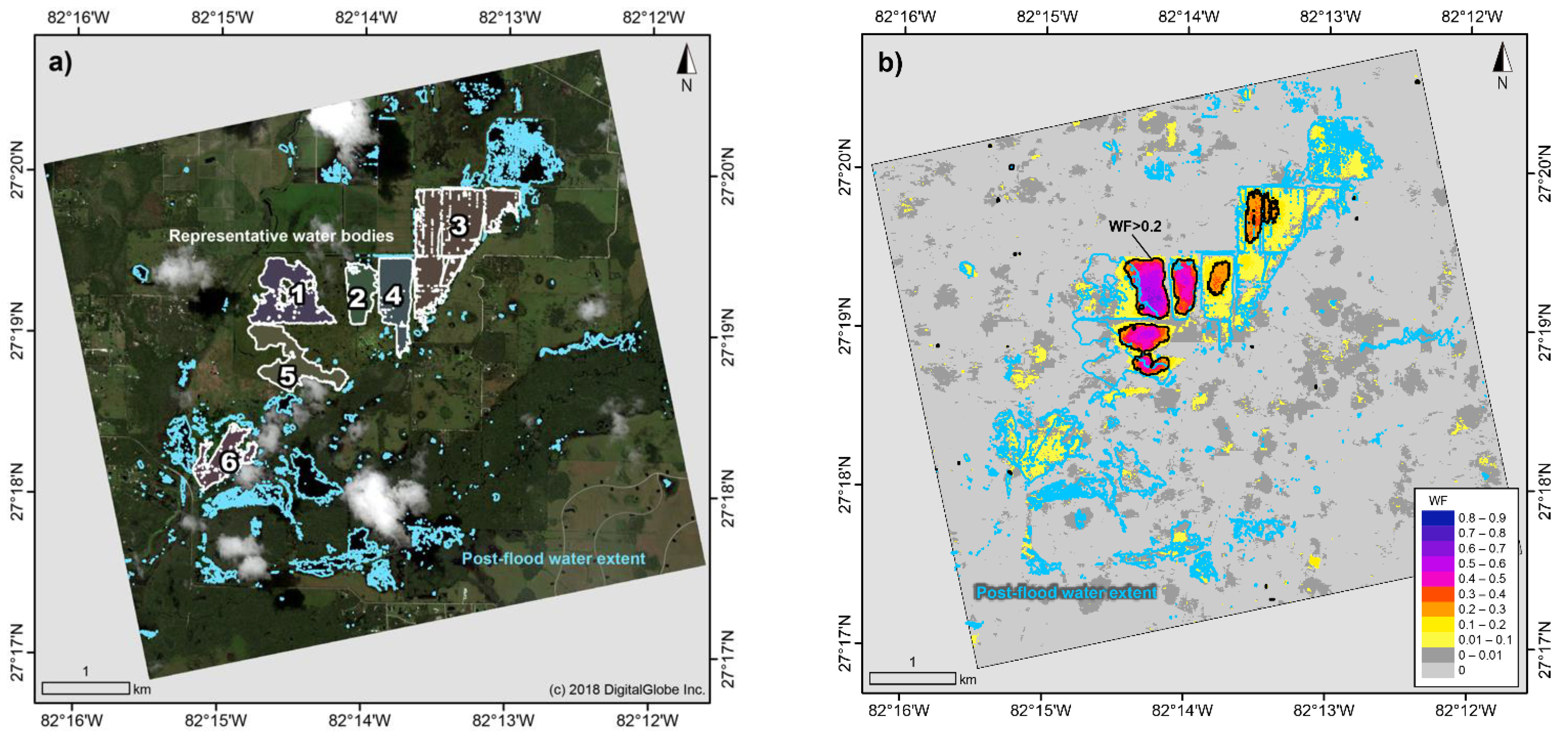
5.1. Optical Water Mapping for Reference

Most parts of the post-flood water bodies in the study site are correctly extracted from the WV2-derived NDWI image and can be observed in visual comparison with the WV2 true color image (Figure 3a). More than six relatively large water bodies (ID numbers attached) and many smaller areas have been extracted. Some rather smaller portions (~10 m) of the water bodies are excluded, probably due to the mixed-pixel effect. Subsequent S2 and SAR data have larger pixel sizes than compared to these small water bodies; therefore, this exclusion does not affect the research objectives.

Potential water bodies, which are not related to hazardous conditions, are obtained by stacking the S2-NDWI images and quantifying the frequency of the presence of water bodies per pixel (0–100%) (Figure 3b). There are several locations with high WF values above 0.2 (indicated by the black outlines in Figure 3b), and slightly lower values are distributed around them. These locations are also covered by water during floods and correspond to the water areas of ID:1–6 (Figure 3a). Therefore, these locations are likely to be potential water bodies (lakes and/or ponds) with some area fluctuation. Scattered portions showing 0–0.01% values of WF (in darker gray) are distributed homogeneously in the study site. These do not correspond to post-flood water-body distribution and potential land cover.

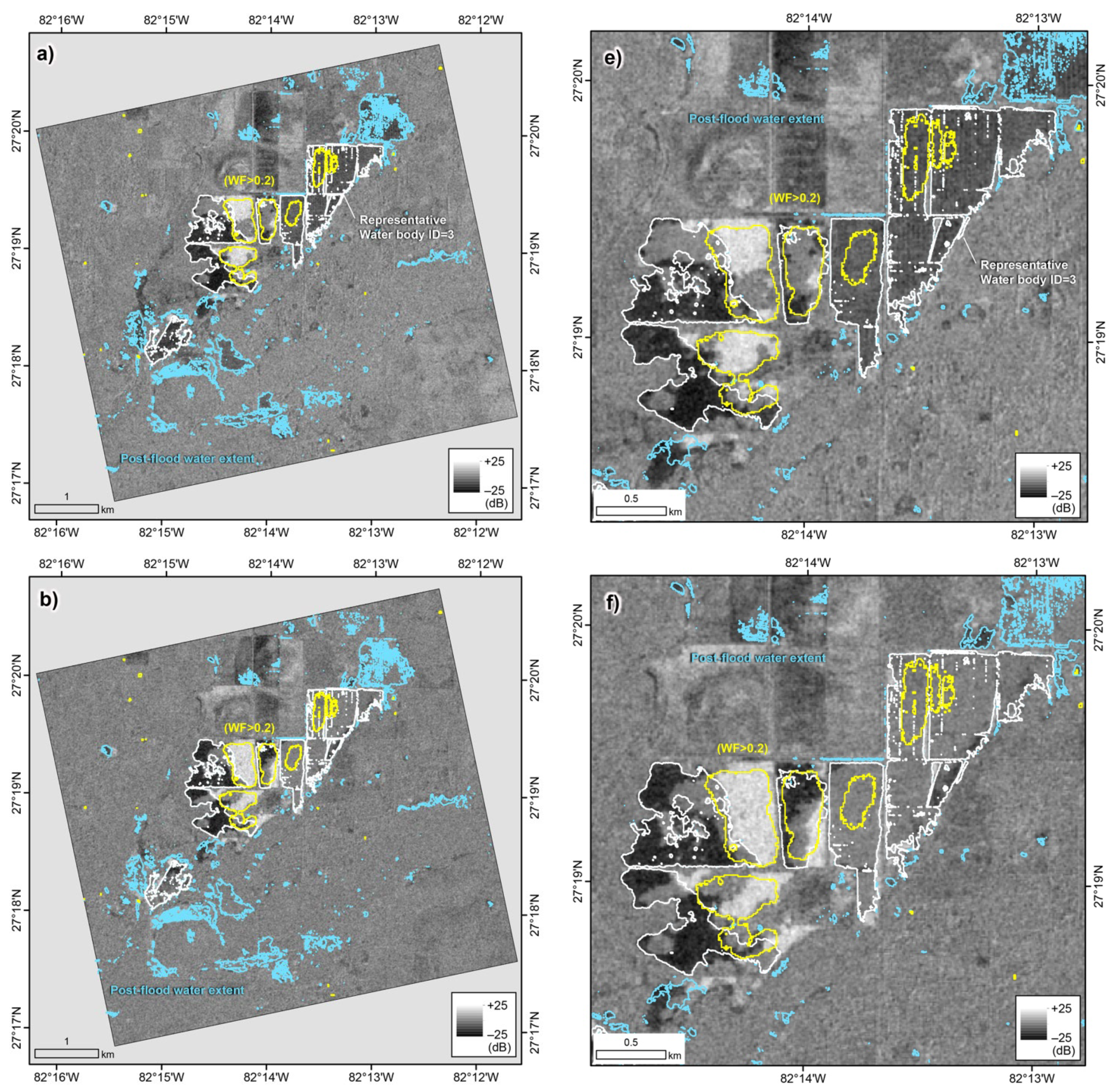
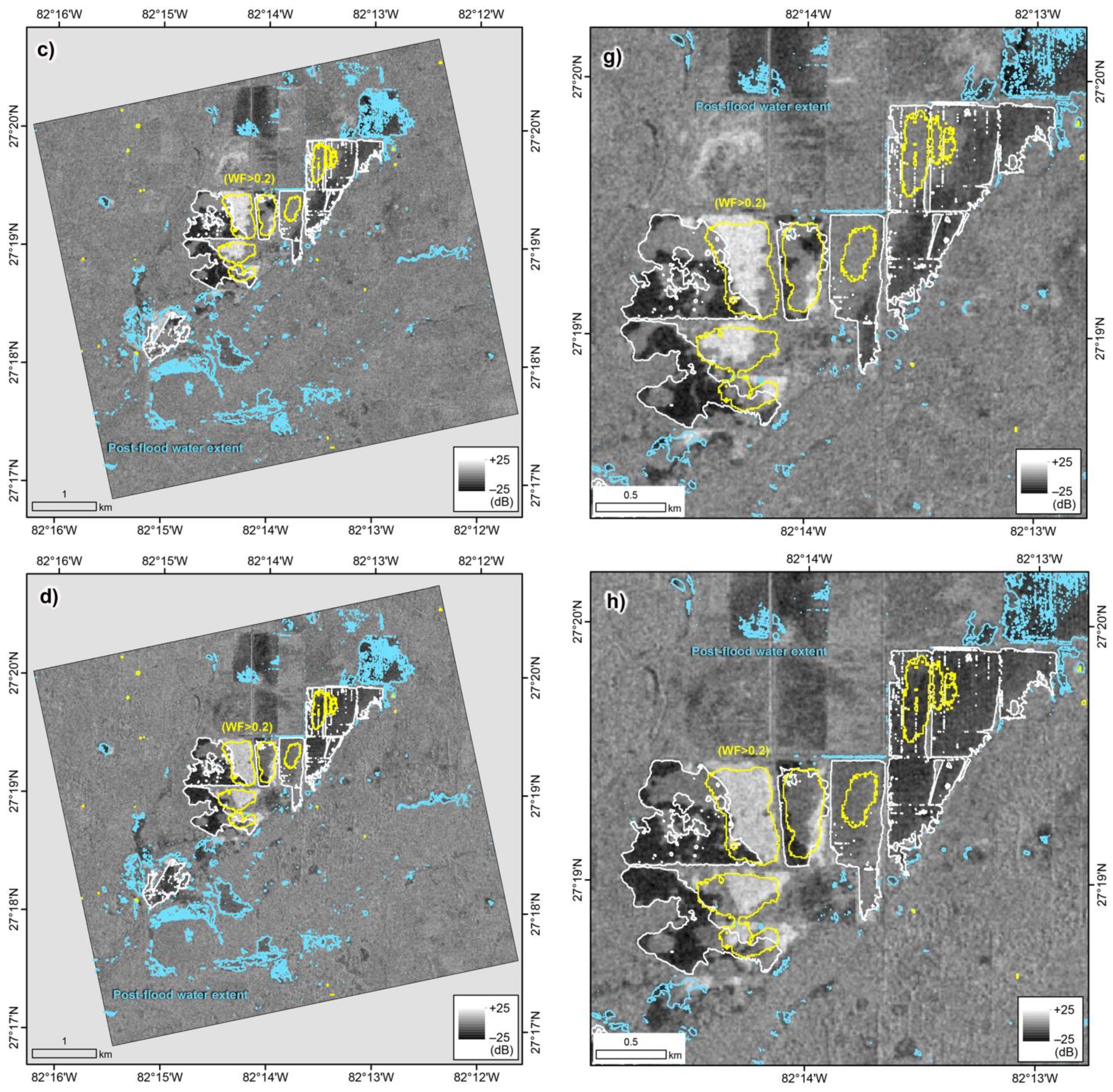
5.2. Single Post-Flood SAR Imagery

Simple visual interpretation of a post-flood SAR image suggests spatial distribution of post-flood water bodies, including potential water extent. Color composite images of PALSAR-2(Figure 4a) and S1 (Figure 4b) dual polarizations denote multiple domains in blue, which is emphasized by their flat surface with smaller volumetric scatter as same as smaller backscatter. Some of these extents correspond to WV2-derived post-flood water distributions (blue outlines as same as Figure 3). The PALSAR-2 image has higher contrast and has easy to visually identify flat surfaces (in blue) than compared to the S1 image. On the other hand, the S1 image emphasizes water bodies that have been identified by WV2 data (blue outlines).

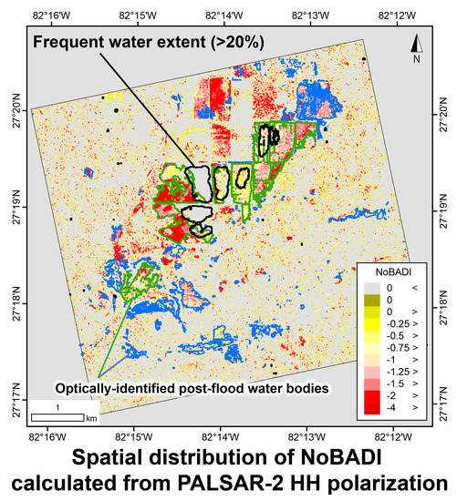
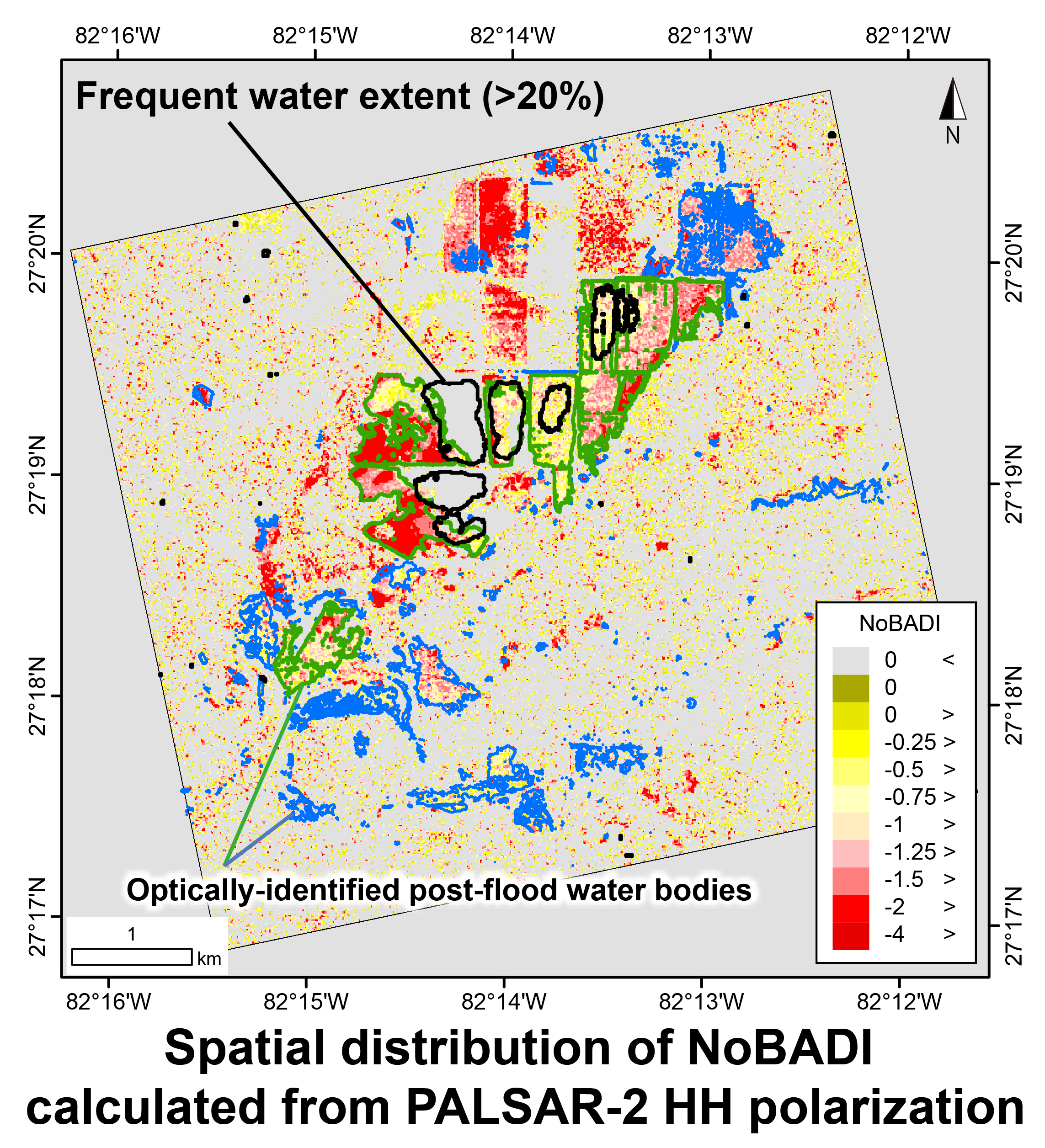
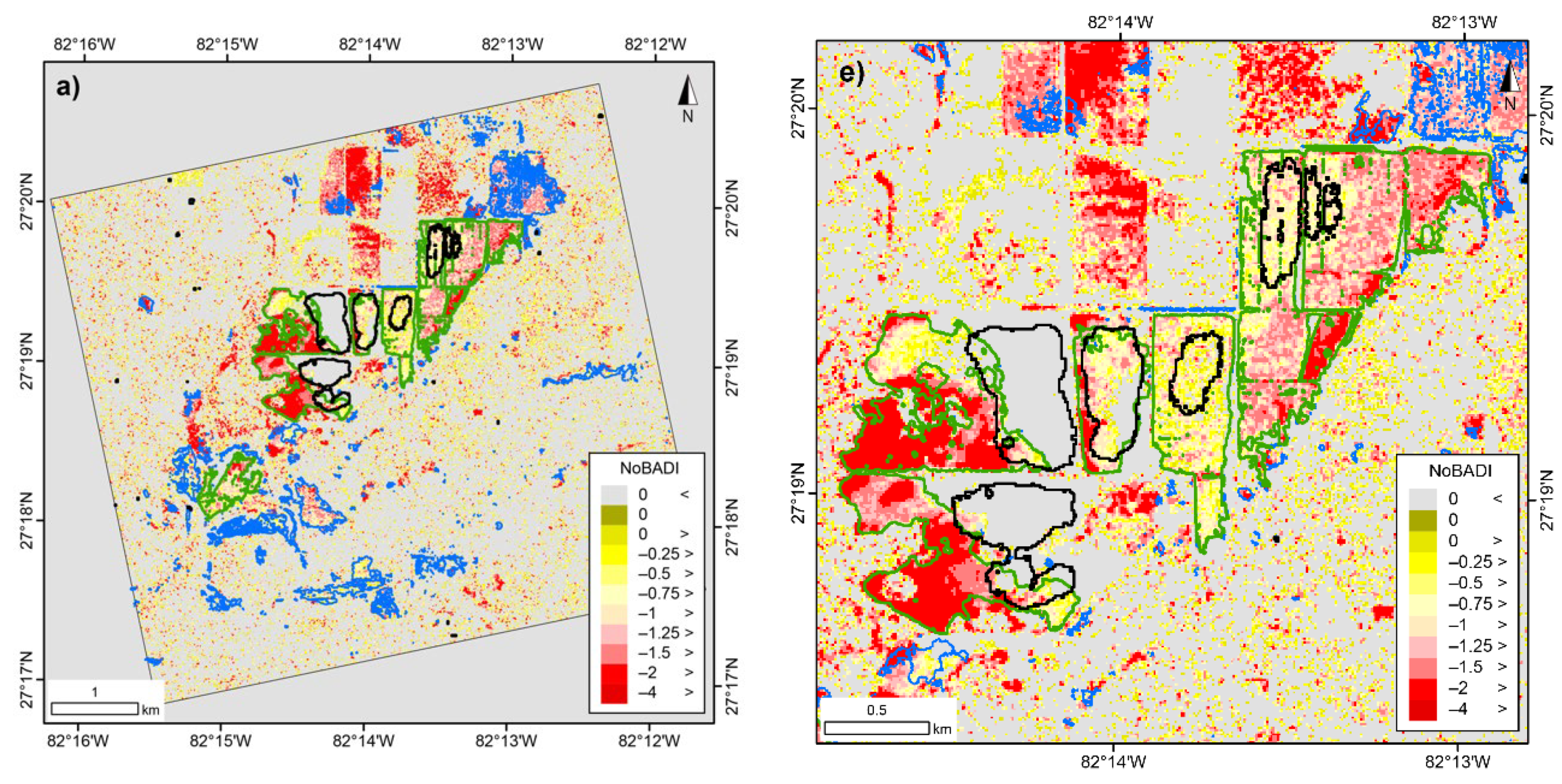
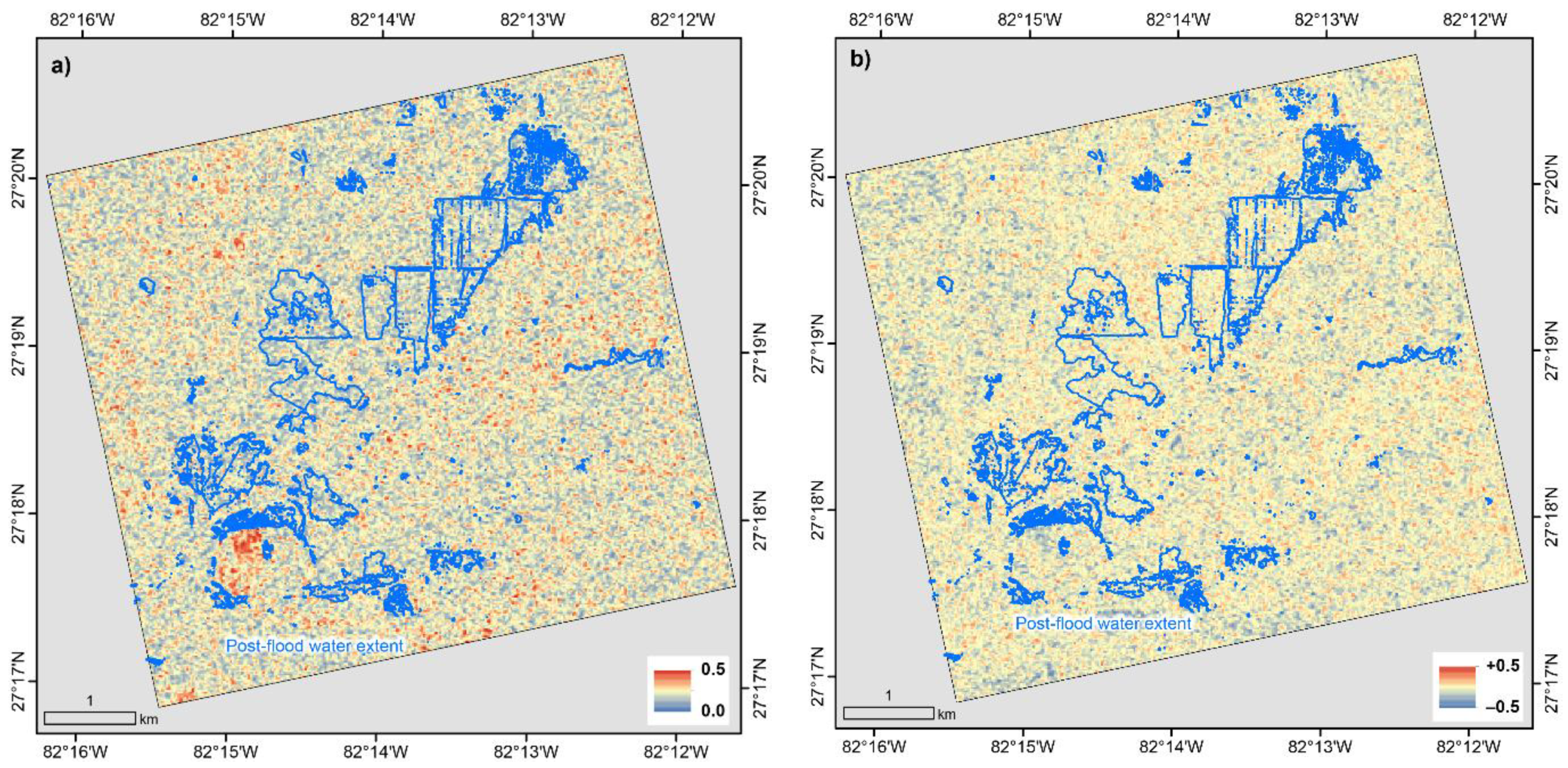
5.3. NoBADI

Spatial distributions of NoBADI in the study site were calculated from PALSAR-2 HH (Figure 5a) and HV (Figure 5b) polarizations as well as from S1 VV (Figure 5c) and VH (Figure 5d) polarizations, respectively. All images show higher values (zero or greater) that are mostly outside the WV2-derived flood portions (in blue/white outlines), whereas the majority of negative values are distributed inside the flood portions. These trends are not influenced by the difference of SAR wavelength (C-/L-bands), polarization (HH, HV, VV, and VH), and stacked number (4 or 143 scenes) of pre-flood images.

In the close-up panels (Figure 5e–h) centered on the representative major flood portions, it can be observed that high values close to zero are distributed in the frequent water areas (>20%) (in black outlines), while lower negative values (<−1) are distributed in the peripheral areas (green/blue) within the post-flood water bodies. These results indicate that NoBADI values generally have lower negative values only in HWE, avoiding potential water extents.

Several parts located at the central north edge of the study site denoted significantly lower values (in light blue) in terms of PALSAR-2 results (Figure 5a,b), which are not shown in S1 results (Figure 5c,d). These locations are not optically referenced in the WV2 true-color image (Figure 3a) because they correspond to cloud shadows. The presence of the water bodies was expected in the PALSAR-2 image (Figure 4a) but not in the S1 image (Figure 3b). Based on this limited information, it is possible that the water body here has decreased between the two observation dates, which may be the reason for the difference in NoBADI results.

5.4. Pre–Post Difference

In order to evaluate the NoBADI results, simple before/after differences in the amplitude of SAR backscatter were calculated for each polarization of PALSAR-2 HH (Figure 6a), HV (Figure 6b), S1 VV (Figure 6c), and VH (Figure 6d). Backscatter amplitude is small in flat surfaces such as water and paved roads. Darker pixels would indicate a severe decrease in backscatter (e.g., flood inundation), while brighter pixels would indicate a severe increase in backscatter (e.g., loss of water extent).

Dark regions should, therefore, correspond to flood-derived water extents. However, their distribution does not correspond to potential water extents (outline in yellow). Fundamentally, their spatial distribution is not homogeneous in the pre-flood water extent (blue/white outlines) among the four images that are visually identifiable in the closed-up panels (Figure 6e–h). Inside a representative water body of ID-3, for example, flood-derived water extent was suggested in the largest area based on the conditions of 19 January 2016 (Figure 6g) and 30 August 2016 (Figure 6h), whereas it was slightly suggested based on the condition of 20 January 2015 (Figure 6e). Based on the condition on 1 September 2015 (Figure 6f), relatively moderate and partial flooding is expected.

The comparison of the most recent month does not ideally match the distribution of the reference water extent. Irregular changes in potential water bodies and not seasonal differences are dominant in the study area. This result suggests that selecting the most recent month’s data as a reference does not always result in accurate water extraction from simple before/after differences.

5.5. Coherence

Multiple previous studies focused on coherence and other InSAR-derived results for flood mapping. The spatial distributions of PALSAR-2 coherence between post-flood (12 September 2017) and pre-flood (30 August 2016) scenes (Figure 7a) and coherence decrease versus two pre-flood scenes (30 August 2016 and 19 January 2016) (Figure 7b) were calculated. The two results do not show any visually identifiable features, and even pre-flood water bodies are difficult to extract. These results suggest that background coherence is generally low in this study area. This may be due to the relatively active growth of vegetation in the tropics and the disturbance of the physical properties of the ground by frequent rainfall over one year.

6. Discussion

6.1. Overview of NoBADI

In this study, a simple function of combining multiple SAR backscatter amplitude data, named NoBADI, was applied to hurricane-induced flood conditions in the study site where the water bodies potentially fluctuate. Single use of pre-flood data would derive different results according to the pre-flood conditions, whereas NoBADI has higher potential to exclude potential water bodies through the statistical algorithm. No significant difference was found between L-band and C-band observations. Indeed, hundreds of pre-flood data, as demonstrated with S1 data, support higher reliability of output information than small samples. According to the result of NoBADI calculated from PALSAR-2 data, however, four pre-flood data, at least, enable the correct output of NoBADI.

Detailed interpretation suggests slightly different characteristics of L-bands/C-bands in terms of volumetric scatter. As described in the Results section, the PALSAR-2 post-flood single image had higher contrast and flat surfaces that were easier to identify than the S1 image. On the other hand, the S1 image emphasizes water bodies, which have been identified by WV2 data. A major reason for the lower contrast for non-water flat domains in S1 data is possibly the difference of L-bands/C-bands. By comparing the two wavelengths, C-band is largely influenced by short grass and coarse vegetation (i.e., volumetric scattering).

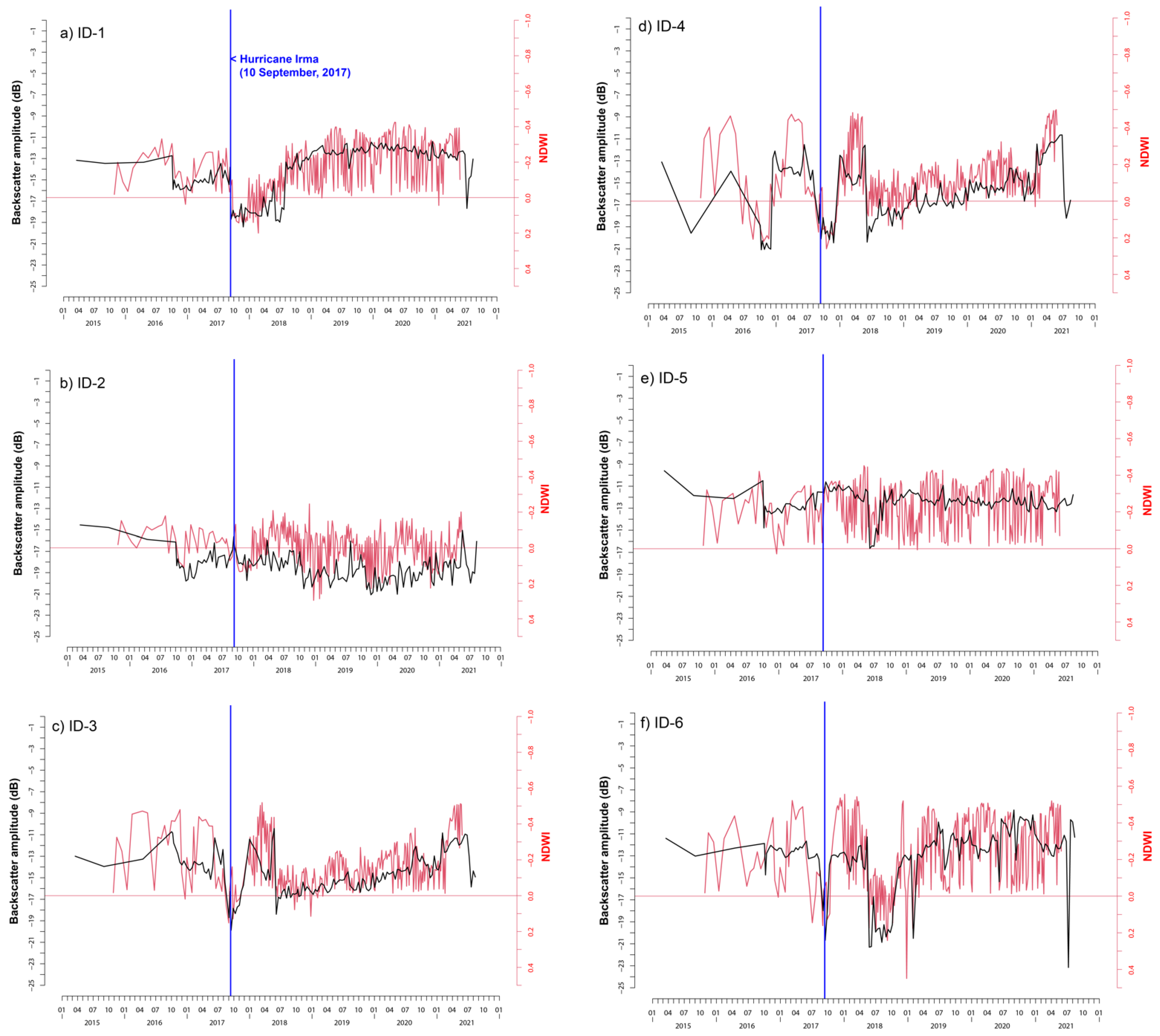
6.2. SAR Backscatter Amplitude and Water Extent

To understand the sensitivity of backscatter amplitude relative to temporal changes of a water-covered area, we compared the relationship between the S1-derived backscatter amplitude (VV) and the S2-derived NDWI in temporal profiles (Figure 8). Each panel corresponds to the domains of representative post-flood water body from ID-1 to ID-6. The backscatter amplitude is negatively correlated with the water extent represented by the average NDWI value for the six domains. This means that backscatter amplitude is a highly sensitive proxy for water existence.

A detailed comparison shows that when the backscatter amplitude is below -16 dB, the NDWI is positive (most of the area is covered by water). The ID-2 domain has a significant drop of backscatter amplitude on September 2016. This means that the land surface turns into a water surface, possibly artificially. The ID-5 domain has mostly positive NDWIs, suggesting land cover in the long term. This domain was temporarily covered by water in response to Hurricane Irma during mid-September 2017, but it is not reflected in the profile possibly due to rapid recovery.

For all profiles, there is no uniform seasonal variation. It was not seasonal changes but transient and irregular events that were dominant for water extent changes. NDWI values have frequent and wide-range fluctuations compared to backscatter amplitude. This is because cloud mask is not applied on this analysis due to statistical limitations. However, we observe that the general trend is the same as in backscatter amplitude.

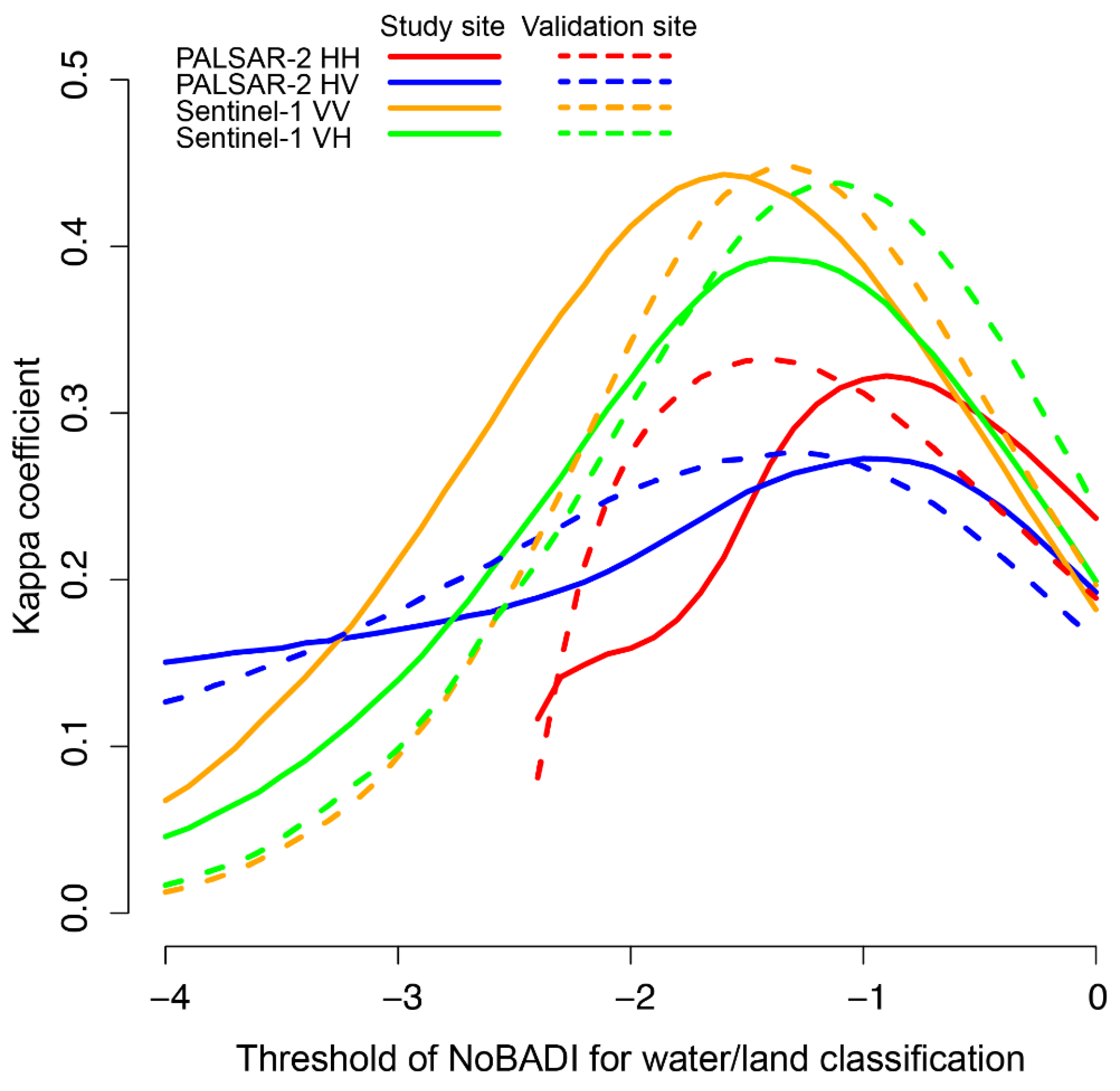
6.3. Optimization of Threshold Value for NoBADI Water Extraction

In the NoBADI analysis, one threshold value is set for binarization, then pixels with lower values are considered flood-derived water extent. Classification accuracy is evaluated by matching NoBADI-derived water pixels versus S2-derived water pixels above the WF of 0.2. In this accuracy validation, the Kappa coefficient is calculated by setting the NoBADI threshold (th.) to multiple values from −4 to 0.

Variations of the Kappa coefficient corresponding to multiple NoBADI threshold are obtained from PALSAR-2 HH, HV, S1 VV, and VH datasets (Figure 9). The highest coefficient value is 0.43 (th. = −1.6) on S1/VV scenes, followed by 0.39 (th. = −1.4) on S1/VH scenes. PALSAR-2 results derive lower maximum coefficients of 0.32 (th. = −0.9) on HH scenes and 0.27 (th. = −1.0) on HV scenes. Selecting these thresholds enables the most optimized extraction of flood-derived water extent. S1 will derive more than PALSAR-2, but PALSAR-2 has more flexible observation criteria for emergency observation under international partnerships. The choice of which one to use will be determined by the timing of observations after the disaster occurs.

To assess sensitivity of the Kappa coefficient, the same calculation was performed for the validation site (see Figure 1). The highest coefficient value is 0.45 (th. = −1.3) on S1/VV scenes, followed by 0.44 (th. = −1.2) on S1/VH scenes. PALSAR-2 results derive lower maximum coefficients of 0.33 (th. = −1.4) on HH scenes and 0.28 (th. = −1.3) on HV scenes. The study site and the validation site, thus, have different values for optimized threshold, which have smaller differences in S1 than PALSAR-2. The S1/VH scenes have values of the Kappa coefficient above/below 0.4, but the VV scenes have similar values both above 0.4 between the two sites. The sensitivity of Kappa coefficient demonstrated in the two sites suggests that S1/VV scenes derive relatively robust outputs that are slightly influenced by selecting the area for analysis.

6.4. Advantages of NoBADI

Fundamentally, the NoBADI method, as we demonstrated in Florida by means of C-band and L-band SAR, is not affected by cloud cover and that supports urgent and promising observation just after or even during the effects of the hurricane. Figure 5 shows the comprehensively similar features of NoBADI’s spatial distribution, although detailed differences are caused among C-bands/L-bands and HH/HV/VV/VH polarizations. Other SAR sensors such as Radarsat-2, NISAR, ALOS-4, and upcoming ones onboard commercial small satellites can potentially apply this method. Note that the X-band has not been verified at this time, so it is expected to be evaluated in the future.

Figure 6 shows that spatial distributions of backscatter amplitude decreasing over the flood event are different depending on the scene that is used as the pre-flood condition. These differences that happen to occur are especially significant within the post-flood water extents, except stable water extents (WF > 0.2) (i.e., HWE). Furthermore, Figure 8 shows that SAR backscatter amplitude and NDWI are irregularly fluctuated and not related to the seasonal cycle. It is possible that the dominant factor here is not the overall seasonality but the uneven cycle of precipitation and evaporation. This suggests that selecting a pre-flood scene in the same season as a post-flood scene does not necessarily improve the uncertainty.

The NoBADI value is not a physical value directly corresponding to backscatter amplitude (dB) but an index that expresses how rare the water extent is. Water extents in a location sometimes covered by water would denote moderate values near zero because standard deviation is relatively large due to frequent changes of land cover. On the other hand, water extents caused in surfaces with small opportunities of water cover would have significantly lower values, which is highlighted in the NoBADI map. For these reasons, spatial distributions of NoBADI (Figure 5) do not denote homogeneous values in the entire surfaces of the HWE. Instead, we can selectively recognize rare water extents as significantly lower NoBADI values.

6.5. Toward Operational Use of Crisis Response

Recent studies of SAR-based flood monitoring analyzed multi-temporal scenes acquired in their study sites [19,20]. Complicated and highly technical methods, however, need to be evaluated in terms of their applicability for each flood case in different topographies and the limitation of available SAR data archives. Our study proposes a simple function of NoBADI aiming to be a standard method for low and flat topography. We conclude that different wavelengths, different polarizations, and the number of pre-flood scenes have certain effects on the output results. These characteristics should be considered for practical applications in crisis response.

NoBADI results do not show neighboring and homogeneous distribution of pixel values for the HWE, but denser and lower pixel values with some deviations around expected places of the HWE (Figure 5). It is possibly the reason why values of the Kappa coefficient are relatively small values that are not larger than 0.5. This may have some difficulties for simple conversion to vector-format polygons. Therefore, further geoinformatics consideration would be needed, such as filter processing and segmentation. Thus, in the present status, NoBADI should be used for the purpose of narrowing down the target area in the first stage of operational use during crisis response. It would be followed by further rigorous analysis in order to collect more accurate information.

7. Conclusions

This study assessed Hurricane-induced Water Extent (HWE) by using SAR-based method of NoBADI and considering the potential fluctuation of water extent in Florida. Both of L-band and C-band SAR data extracted flood-derived water while excluding potential water distribution. These wavelengths can be used to obtain initial information about the flood distribution, and the classification accuracy is higher in the C-band. Future studies will be expected for the validation of NoBADI analysis in other locations that have different temporal patterns of water surface fluctuation.

References

- Agnihotri, A.K.; Ohri, A.; Gaur, S.; Shivam; Das, N.; Mishra, S. Flood inundation mapping and monitoring using SAR data and its impact on Ramganga River in Ganga basin. Environ. Monit. Assess. 2019, 191, 760. [Google Scholar] [CrossRef] [PubMed]
- Bayik, C.; Abdikan, S.; Ozbulak, G.; Alasag, T.; Aydemir, S.; Sanli, F.B. Exploiting multi-temporal Sentinel-1 SAR data for flood extend mapping. In Proceedings of the International Archives of the Photogrammetry, Remote Sensing and Spatial Information Sciences—ISPRS Archives, Istanbul, Turkey, 18–21 March 2018; Volume 42. [Google Scholar]
- Sanyal, J.; Lu, X.X. Application of Remote Sensing in Flood Management with Special Reference to Monsoon Asia: A Review. Nat. Hazards 2004, 283–301. [Google Scholar] [CrossRef]
- Long, S.; Fatoyinbo, T.E.; Policelli, F. Flood extent mapping for Namibia using change detection and thresholding with SAR. Environ. Res. Lett. 2014, 9, 035002. [Google Scholar] [CrossRef]
- Meyer, F.J.; Ajadi, O.A.; Schultz, L.; Bell, J.; Arnoult, K.M.; Gens, R.; Nicoll, J.B. An automatic flood monitoring service from Sentinel-1 SAR: Products, delivery pipelines, and performance assessment. In Proceedings of the IGARSS 2018—2018 IEEE International Geoscience and Remote Sensing Symposium, Valencia, Spain, 22–27 July 2018; pp. 6576–6579. [Google Scholar] [CrossRef]
- Meyer, F.J.; Ajadi, O.A.; Schultz, L.; Bell, J.; Arnoult, K.M.; Gens, R.; Molthan, A.L.; Nicoll, J.B.; Hogenson, K. Applications of a SAR-based flood monitoring service during disaster response and recovery. In Proceedings of the IGARSS 2019—2019 IEEE International Geoscience and Remote Sensing Symposium, Yokohama, Japan, 28 July–2 August 2019; pp. 4649–4652. [Google Scholar]
- Watanabe, M.; Koyama, C.N.; Hayashi, M.; Nagatani, I.; Tadono, T.; Shimada, M. Refined algorithm for forest early warning system with ALOS-2/PALSAR-2 ScanSAR data in tropical forest regions. Remote Sens. Environ. 2021, 265, 112643. [Google Scholar] [CrossRef]
- Florida State University Florida Climate Center. Available online: https://climatecenter.fsu.edu/ (accessed on 31 January 2021).
- Cangialosi, J.P.; Latto, A.S.; Berg, R. National Hurricane Center Tropical Cyclone Report: Hurricane Irma (30 August–12 September 2017); NOAA National Centers for Environmental Information: Asheville, NC, USA, 2018. [Google Scholar]
- National Aeronautics and Oceanic Administration BULLETIN—Hurricane Irma Intermediate Advisory Number 45A. Available online: https://www.capeweather.com/weather-ftopicp-27027.html (accessed on 31 August 2021).
- Chakalian, P.M.; Kurtz, L.C.; Hondula, D.M. After the Lights Go Out: Household Resilience to Electrical Grid Failure Following Hurricane Irma. Nat. Hazards Rev. 2019, 20, 05019001. [Google Scholar] [CrossRef]
- Mitsova, D.; Esnard, A.M.; Sapat, A.; Lai, B.S. Socioeconomic vulnerability and electric power restoration timelines in Florida: The case of Hurricane Irma. Nat. Hazards 2018, 94, 689–709. [Google Scholar] [CrossRef]
- Feng, K.; Lin, N. Reconstructing and analyzing the traffic flow during evacuation in Hurricane Irma (2017). Transp. Res. Part D Transp. Environ. 2021, 94, 102788. [Google Scholar] [CrossRef]
- Issa, A.; Ramadugu, K.; Mulay, P.; Hamilton, J.; Siegel, V.; Harrison, C.; Campbell, C.M.; Blackmore, C.; Bayleyegn, T.; Boehmer, T. Deaths Related to Hurricane Irma—Florida, Georgia, and North Carolina, September 4–October 10, 2017. MMWR. Morb. Mortal. Wkly. Rep. 2018, 67, 829–832. [Google Scholar] [CrossRef] [PubMed] [Green Version]
- MAXAR Technologies WorldView-2 Datasheet. Available online: https://resources.maxar.com/data-sheets/worldview-2 (accessed on 31 August 2021).
- European Space Agency Sentinel-2 MSI User Guide. Available online: https://sentinel.esa.int/web/sentinel/user-guides/sentinel-2-msi (accessed on 31 August 2021).
- Updike, T.; Comp, C. Radiometric Use of WorldView-2 Imagery Technical Note; DigitalGlobe: Westminster, CO, USA, 2010; pp. 1–17. [Google Scholar]
- McFeeters, S.K. The use of the Normalized Difference Water Index (NDWI) in the delineation of open water features. Int. J. Remote Sens. 1996, 17, 1425–1432. [Google Scholar] [CrossRef]
- Uddin, K.; Matin, M.A.; Meyer, F.J. Operational flood mapping using multi-temporal Sentinel-1 SAR images: A case study from Bangladesh. Remote Sens. 2019, 11, 1581. [Google Scholar] [CrossRef] [Green Version]
- Martinis, S.; Rieke, C. Backscatter analysis using multi-temporal and multi-frequency SAR data in the context of flood mapping at River Saale, Germany. Remote Sens. 2015, 7, 7732–7752. [Google Scholar] [CrossRef] [Green Version]
Publisher’s Note: MDPI stays neutral with regard to jurisdictional claims in published maps and institutional affiliations. |
© 2021 by the authors. Licensee MDPI, Basel, Switzerland. This article is an open access article distributed under the terms and conditions of the Creative Commons Attribution (CC BY) license (https://creativecommons.org/licenses/by/4.0/).
Share and Cite
Nagai, H.; Abe, T.; Ohki, M. SAR-Based Flood Monitoring for Flatland with Frequently Fluctuating Water Surfaces: Proposal for the Normalized Backscatter Amplitude Difference Index (NoBADI). Remote Sens. 2021, 13, 4136. https://doi.org/10.3390/rs13204136
Nagai H, Abe T, Ohki M. SAR-Based Flood Monitoring for Flatland with Frequently Fluctuating Water Surfaces: Proposal for the Normalized Backscatter Amplitude Difference Index (NoBADI). Remote Sensing. 2021; 13(20):4136. https://doi.org/10.3390/rs13204136
Chicago/Turabian StyleNagai, Hiroto, Takahiro Abe, and Masato Ohki. 2021. "SAR-Based Flood Monitoring for Flatland with Frequently Fluctuating Water Surfaces: Proposal for the Normalized Backscatter Amplitude Difference Index (NoBADI)" Remote Sensing 13, no. 20: 4136. https://doi.org/10.3390/rs13204136
APA StyleNagai, H., Abe, T., & Ohki, M. (2021). SAR-Based Flood Monitoring for Flatland with Frequently Fluctuating Water Surfaces: Proposal for the Normalized Backscatter Amplitude Difference Index (NoBADI). Remote Sensing, 13(20), 4136. https://doi.org/10.3390/rs13204136