Abstract
Spaceborne synthetic aperture radar (SAR) represents a powerful source of data for enhancing maritime domain awareness (MDA). Wakes generated by traveling vessels hold a crucial role in MDA since they can be exploited both for ship route and velocity estimation and as a marker of ship presence. Even if deep learning (DL) has led to an impressive performance boost on a variety of computer vision tasks, its usage for automatic target recognition (ATR) in SAR images to support MDA is still limited to the detection of ships rather than ship wakes. A dataset is presented in this paper and several state-of-the-art object detectors based on convolutional neural networks (CNNs) are tested with different backbones. The dataset, including more than 250 wake chips, is realized by visually inspecting Sentinel-1 images over highly trafficked maritime sites. Extensive experiments are shown to characterize CNNs for the wake detection task. For the first time, a deep-learning approach is implemented to specifically detect ship wakes without any a-priori knowledge or cuing about the location of the vessel that generated the wake. No annotated dataset was available to train deep-learning detectors on this task, which is instead presented in this paper. Moreover, the benchmarks achieved for different detectors point out promising features and weak points of the relevant approaches. Thus, the work also aims at stimulating more research in this promising, but still under-investigated, field.
1. Introduction
In recent years, the improvement of maritime domain awareness (MDA) is assuming a crucial role in achieving effective maritime security, border control, environmental protection of marine protected areas (MPA) and the control of illegal, unreported and unregulated (IUU) fishing and law enforcement systems. However, the future enhancement of MDA will demand collecting and merging terabytes (TB) of data coming from several different sources (e.g., land, sea-based, airborne and spaceborne sensors). Currently, the most exploited system for maritime monitoring is the automatic identification system (AIS), whose requirements have been regulated by the international maritime organization (IMO) [1]: medium and large ships (>300 tons) have to carry the AIS transmitter to communicate data regarding its identification and route information. However, the AIS transmitter can be deliberately turned off. In such a case, the ship becomes a “dark vessel”, i.e., ship operating without an AIS transponder or even with this device switched off [2]. With this regard, both ongoing projects [3] and data providers [4] are focusing resources towards the detection of dark vessels by integrating AIS data and information acquired by synthetic aperture radar (SAR) images [5,6,7,8]. Results confirm the satellite technologies as a key solution providing support and improving the current capabilities of existing maritime monitoring systems, thanks to the large amount of available data. For instance, more than 12 TB are produced each day by Sentinel missions [9]. Recent studies [10] have shown that the detection, recognition and reconstruction of the ship wake can strongly contribute to the improvement of MDA, since the wake (a) provides additional information about the route, i.e., ship velocity and heading, and (b) enables the detection of ships not imaged in SAR images due to their motion, materials and sizes. The traditional approaches for wake detection in SAR images assume a wake structure basically composed by linear features, i.e., the turbulent wake, two narrow-V wakes and the Kelvin pattern, appearing as bright and dark lines [11]: the detection problem is thus typically challenged with domain transforms such as Radon [5] or Hough. However, wakes can assume very different appearances depending on the ship speed, hull shape, orientation (range and azimuth), sea condition and wind speed, radar signal wavelength and observation geometry, but also their appearance can be very similar to that resulting from different phenomena, like sea surface films and oil spills [12].
With its ability to automatically glean patterns from data, deep learning (DL) has generated an international hype in the space sector in general, and for remote sensing in particular. Concerning SAR applications, DL architectures have been applied for numerous tasks including despeckling [13], SAR-optical image fusion [14] and automatic target recognition (ATR) [15]. More in depth, the research activities about ATR for maritime surveillance have been mainly focused on the ship detection problem by convolutional neural networks (CNNs), proving better accuracy at less test cost [16,17]. Furthermore, in the wake-detection field, the DL-based methods can arguably be a promising choice, since they well address the problem of generalization and benefit of HPC (high-performance computing) architectures with clusters of GPUs. The various wake appearances can be properly addressed in various environments and maritime weather conditions thanks to the capability of “supervised learning”. To the knowledge of the authors, no deep learning architecture dedicated to wake detection in SAR images has been developed yet. The only results published in the literature [18] adopt a CNN classifier to detect ship wakes from TerraSAR-X images for route estimation purposes. Hence, it is applied only for wakes close to a well distinguishable ship in X-band imagery. Besides, their approach to achieve object detection constrains to use a significant number of region proposals and, thus, is computationally inefficient. The problem can be bypassed by state-of-the-art object detectors, which utilize anchor boxes for the automatic search of instances [19].
The contribution of the paper to DL-based wake detection is thus two-fold: (i) discussing the main properties of existing DL-based object detectors, and (ii) showing the first application of DL-based wake detection conceived to recognize ship wakes in SAR images. To achieve the former, an SAR Ship Wake Dataset (SSWD) has been properly built and detailed, representing an additional original contribution of this work and paving the way to open discussions in the scientific community. The paper is organized as follows: Section 2 shows an overview of the most mature DL-based detectors, Section 3 introduces the complexity of wake visibility and detectability, Section 4 details the dataset, Section 5 described the setup and the metrics used in Section 6 to assess the performance of the DL architectures both on the SSWD and on C- and X-band products.
2. Selected Object Detectors
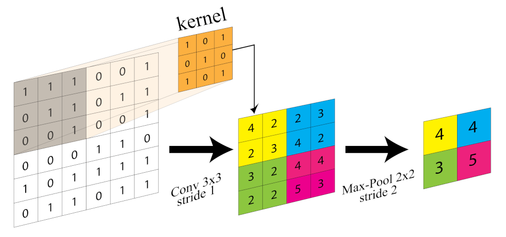
Convolutional neural network (CNN, or ConvNet) is a deep neural network well-suited for visual tasks. They are a type of feed-forward artificial neural network (ANN) with variations of multilayer perceptrons designed to use minimal amounts of preprocessing. CNNs have been successfully applied to numerous computer vision tasks, such as classification, semantic segmentation, and object detection. In 2012, AlexNet [20] won the ImageNet competition on the classification task. Since then, CNN architectures have drawn huge interest due to their capability of gleaning low-, mid- and high-level features stacking together convolutional and pooling layers (Figure 1).

Figure 1.
Convolution (kernel size 3 × 3 and stride 1) and Pooling (kernel size 2 × 2 and stride 1) layer illustration.
After AlexNet, more complex and sophisticated networks followed, such as ZF-Net [21], VGG-Net [22], GoogLeNet (Inception v1) [23], and ResNet [24]. However, the encoder architecture only allows one to perform the classification task: to achieve object detection the CNN architecture must be broadened. Object detection is the visual task that aims at recognizing instances of a predefined set of classes (e.g., ship, wake, oil spill) and accurately locates them in the image with bounding boxes. A naive approach to achieve object detection is to tile different Regions of Interest (RoIs) from the starting image and use of a CNN to classify the presence of the object within that region. In this way, the object detection problem is rearranged as a classification problem. Notably, the detectors using this approach are referred to as two-stage detectors, since the detection process is devised in two steps. Anyway, since objects might have different spatial locations and aspect ratios, this solution forces selection of a huge number of RoIs at the expense of a high computational burden. Girshick and Ross put their strengths into the object detection task, introducing the region-based convolutional neural network (R-CNN or regions with CNN) [25]. Compared to traditional methods, R-CNN greatly improved the results on the Pascal VOC dataset [26]. The advantage of R-CNN is using only 2000 RoIs (or region proposals), generated using a greedy algorithm called “selective search”. After region proposal generation, RoIs are warped into a square, fed into the CNN and then an SVM (support-vector machine) classifies the extracted features to locate the presence of the object within the candidate RoI. Still, this algorithm requires a significant amount of time for training and testing, making it hard to apply in the industry. To solve this problem, numerous improvements of R-CNN followed, enabling better performance at a less computational cost. The most recent ones are semi-supervised object detectors (SS-ODs) [27,28], which exploit both labeled and unlabeled data. These make use of pseudo-labels to perform a feature distillation with guided contrastive learning in a mutual teacher-student fashion. Since these approaches extend the default detection frameworks, the latter are described in the next sub-sections, and applied to the proposed dataset.
Concluding this section it is important to point out that the recent literature has shown completely different schemes which are anchor-free [29,30,31] or transform-based [32,33,34]. However, these will not be analyzed in this first assessment.
2.1. Two-Stage Detectors
The evolution of R-CNN detectors is referred to in the literature as an R-CNN family. Hereinafter, the developments from Faster R-CNN to Mask R-CNN and Cascade Mask R-CNN are detailed.
2.1.1. Faster R-CNN
The same authors of R-CNN lately proposed Faster R-CNN [19]. The bottleneck of the region proposal computation is tackled by a region proposal network (RPN), i.e., a fully convolutional network trained to generate region proposals. RPN indeed predicts RoIs from the feature map generated by the backbone using anchor boxes. These are a set of bounding boxes having predefined width and height. Anchors are defined to capture the scale and aspect ratio of specific objects. Then, the proposed RoI pooling layer takes every RoI and linearly downscales them to the size of the feature map. Finally, that feature map section is converted into a fixed dimension map. It is worth noting that the size of the feature map is reduced after the convolutional and pooling layers. This solves the major hurdle of object detection: fully connected (FC) layers set a fixed input size requirement to the network. As a result, the same feature map is used for all the proposals, thus allowing one to pass the entire image to the CNN instead of each proposal individually. This architecture classification is not more executed by an SVM for each class but through a single softmax layer [35]. Indeed, the architecture holds two different outputs. The first one being a discrete probabilistic distribution of anchor belonging to classes. As mentioned, is obtained through a softmax function prompted on the outputs of the FC layer. The other outputs are the bounding box coordinates fitted by the bounding box regressor [19].
As the learning process in DL is cast as an optimization problem, a loss function must be defined for calculating the error of the model during the supervised learning process. The loss function resembles the model performance in one scalar number, which allows candidate solutions to be ranked. The loss function associated with each extracted RoI, is set as in [19]:
where is the normalization term set to the mini-batch size (i.e., the number of samples from the dataset used for training one epoch), is the normalization term set number of anchors while is a coefficient setting the relative importance between and in the determination of the loss function.
The loss function associated with the classifier is:
with denoting the ground truth (binary) of whether the anchor is an instance or not. Instead, the loss function relative to the regressor is equal to:
in which is the smooth L1 loss defined as:
It is worth noting that Equation (1) defines a multi-task loss function, which considers both the classification and the bounding box regression results. This implementation brushed up detection speed and accuracy [19] and has shown impressive results on a variety of computer vision tasks, providing a network foundation with high detection accuracy.
2.1.2. Mask R-CNN
Two years later, Mask R-CNN [36] was developed by Facebook AI Research (FAIR). Mask R-CNN was based on Faster R-CNN and outperformed all existing single-model entries (at that moment) on every task, including the COCO 2016 challenge winners [36]. Mask R-CNN further extends the capabilities of Faster R-CNN, adding a branch for generating a high-quality segmentation mask for each RoI. The mask branch (Figure 2) operates in tandem with the classifier and bounding box regressor.
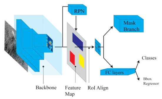
Figure 2.
Mask R-CNN architecture illustration.
This FC network processes each RoI, outputting a segmentation mask in a pixel-to-pixel manner. Besides, adding only a small computational overhead, the fast detection speed is preserved.
The most evident advantage of Mask R-CNN was its usage of the RoI align layer in substitution of the RoI pooling layer for RoI extraction from the feature map. This solves the coarse spatial quantization problem for feature extraction overcoming the round-off errors due to floating point division. This is done with the proper alignment of the extracted features with the input. Indeed, the RoI align layer utilizes bilinear interpolation to prompt the input feature values at four locations sampled in a regular way for each RoI bin. Then, the result is combined, utilizing average or max operators [36]. For the definition of multi-task loss of Mask R-CNN, the authors of [36] added to the loss function of Faster R-CNN and the loss of a segmentation mask. The loss is therefore formulated as:
The mask branch generates a mask of dimension for each RoI and for each of k classes. Thus, the total output is of size . As stated in [36], there is no competition among classes in mask generation because the model learns masks for each class separately. The is defined by [37], as a binary cross-entropy loss of the average per-pixel sigmoid output over the k dimensions:
where is the label of a pixel, is the ground-truth mask and is the predicted value of the same pixel for the class k [36].
2.1.3. Cascade Mask R-CNN
As a further aspect, there is always a trade-off involved in object detection between detector quality and performance. In this context, quality denotes accuracy of the predicted bounding boxes with reference to the ground truth, while performances are evaluated trough object detection metrics. See Section 5.2 for more details. This trade-off is defined by the intersection over union (IoU) (detailed in Section 5.2). As reported by [38], this issue has two causes. The first one is related to the object proposal mechanism which tends “to produce hypotheses distributions heavily imbalanced towards low quality” [38]. Consequently, large values of IoU thresholds determine a reduction of positive training samples during training. The second one regards the mismatch between detector quality and assumptions available at the inference time [38]. Cascade R-CNN [38] addresses this problem with an architecture built with a sequence of detectors (e.g., Faster R-CNN or Mask R-CNN) trained with increasing IoU thresholds, e.g., {0.5, 0.6, 0.7}. Therefore, this strategy progressively improves the quality of hypotheses, thus acting as a preventive measure against overfitting [38]. In the present paper, the Cascade approach will be tested using Mask R-CNN as detector.
2.2. One-Stage Detectors
In addition to the above-discussed two-stage detectors, one-stage detectors exist, which achieved sufficient quality and performance. Lacking a region proposal step, they are arguably referred as region-free models (RF-models). The lack of a prior task to generate proposals leads to simpler and faster model architectures. In this ambit, RetinaNet [39] is worthy of being mentioned. It is a one-stage object detector, which prevents positive-negative RoI imbalance with a huge number of RoIs and a custom loss function, i.e., focal loss. Focal loss was formally formulated as [39]:
where the cross entropy loss is modulated by the factor with the tunable focusing parameter . The balancing parameter was lately introduced to guarantee slightly improved accuracy [39]. For notation convenience, is defined as:
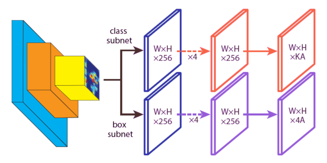
RetinaNet attaches to the backbone of two subnetworks, “one for classifying anchor boxes and one for regressing from anchor boxes to ground-truth object boxes” [39]. The architecture is very similar for the two aforementioned networks but the parameters are not shared. The network design results are very simple, enabling the focal loss function to eliminate the accuracy gap between RetinaNet and state-of-the-art two-stage detectors while running at faster speeds. Figure 3 illustrates RetinaNet subnetworks, in which W, H, and represent the width, height and number of channels of the feature map, respectively. Instead, K denotes the number of object classes, and A the number of anchors [39].

Figure 3.
RetinaNet FCN subnetwork illustration: (top) classification subnet and (bottom) bounding box regression subnet.
2.3. Backbone Network
The baseline detectors used in this work all utilize deep residual network (ResNets) backbones. This is a common choice for dense object detectors and it is done in purpose for comparing the performance of the detectors on the same dataset under the same conditions. ResNet backbones are selected as the main feature extractor, since they are deep but stable. Thanks to their residual building blocks, they represent an effective way to solve the vanishing gradient problem [24]. Their combination with feature pyramid networks (FPN) [40] is another common choice used to construct the “top-down feature pyramid structure fusing the inherent multi-scale feature map” [40]. The composite structure of ResNet and FPN makes the detectors adaptable to detect either small and large objects.
3. Wake Imaging Mechanism
As mentioned in the Introduction, the wake generated by a moving ship shows several components, namely the turbulent wake, narrow-V wake and Kelvin pattern. They are arranged in two fans, the first one composed by the turbulent wake and the narrow-V wake within an aperture of 4°, and second one including the Kelvin features, i.e., transverse, divergent and cusp waves, within an aperture of about 19° [41]. However, the above-described wake structure is not always realized [42], i.e., the V-shape of the wake depends on the Froude number ():
where u is the vessel velocity, g the acceleration of gravity, and L the vessel length at the waterline. In detail, increasing the Froude number, the narrow-V wakes become narrower [43] and the Kelvin pattern modifies so that (i) for Fr < 0.7, i.e., sub-critical conditions, the well-known pattern is shown; (ii) for 0.7 < Fr < 1, i.e., trans-critical conditions, the angle of the divergent waves angle increases; (iii) for Fr > 1, i.e., super-critical conditions, no transverse or cusp waves are present.
Moreover, when the wake is imaged by an SAR, its appearance is dependent on the imaging mechanisms and the detectability of its components are influenced by both radar-related and environmental-related parameters [44]. Indeed, since the turbulent wake is smoother than its surroundings, reflecting less energy back to the radar, it appears as a dark strip in the image. On the contrary, the narrow-V wakes are shown as two bright lines, resulting from Bragg scattering of radar pulses from waves generated by the hull moving through the water. Similarly, the features of the Kelvin pattern are shown as bright features. Regarding the detectability, the turbulent wake is widely recognized as the most distinguishable component with a larger contrast at lower frequencies under moderate wind speeds [45]. Instead, narrow-V wakes are seen only at low-wind speeds (<3 m/s) in deep and shallow water. Concerning the Kelvin pattern, the visibility of all components, that are extremely rare [46], depends on several factors, (i) polarization, with the fan more distinguishable at the horizontal (HH), than at the vertical (VV)-polarized images, (ii) incidence angle, with more pronounced components at steeper angles [47] and (iii) direction of propagation of the waves, which leads to a more visible wake when it is parallel to the radar look direction [46]. Indeed, when waves propagate parallel to the azimuth direction, the velocity bunching [46] effect makes them smeared, thus notably limiting their visibility in the image. Moreover, the Kelvin transverse or cusp wakes can be distinguishable when the image resolution is better than half of their wavelength [48]. As a result, assuming the typical resolution of Sentinel-1 Interferometric Wave mode of about 20 m, the cusps cannot be resolved as an individual wavefront, appearing as a bright border of the Kelvin fan, for ships moving slower than 15 knots.
4. Dataset Description
The developed SAR Ship Wake Dataset (SSWD) includes 261 wake chips (512 × 512 pixels) extracted from Interferometric Wide (IW) swath Sentinel-1 SAR images gathered in vertical transmit-vertical receive (VV) polarization.
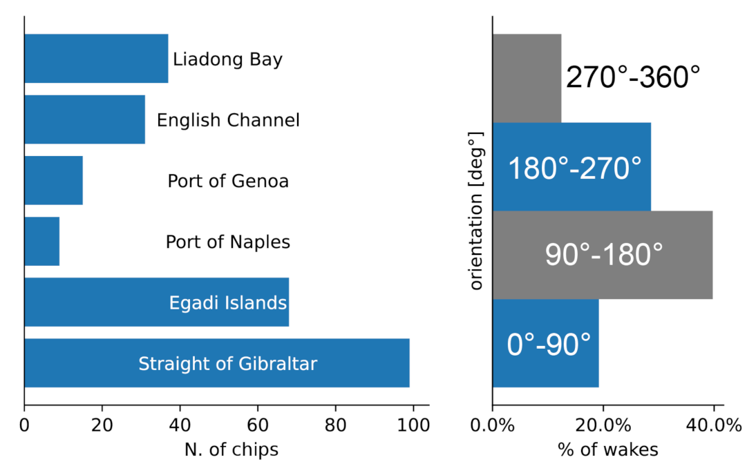
The images were obtained from Copernicus Open Access Hub and correspond to Level-1 ground range detected (GRD) products with a pixel spacing of about 10 m × 10 m (ground range × azimuth). Sites cover highly trafficked maritime sites, like the Strait of Gibraltar, Egadi Islands (Italy), the Gulfs of Genoa and Naples (Italy), the English Channel, and the Liaodong Bay (China). They have been selected for maximizing chip diversity, so to include different ship classes, heading, speed and orientations, that is the moving direction of the ship in the image. Figure 4 (left) summarizes the number of chips acquired in each procurement site of SSWD. The total number of wakes labeled was 291, it is greater than the number of chips since the 12% of chips include more than one wake. Figure 4 (right) also shows the statistical distribution of the wake orientation. The relevant angle is computed counter-clockwise with respect to the ground range direction.

Figure 4.
Statistical distribution of chip wakes across procurement sites (left) and orientation distribution along the four quadrants (right).
It is evident that the dataset shows a balanced behavior: orientations between 0–90° and 180–270° are almost equally represented as the ones between 90–180° and 270–360°. After subsetting, data conversion to 8-bit depth was performed by clipping the histogram (95%) with the SNAP (ESA) toolboxes. To save VRAM (video random access memory) and allow faster training, a size of ∼512 × 512 pixels was chosen for each chip. Significant attention was given to the annotations since a wrong labeling could damage the data veracity. Data labeling was performed with the VIA image annotator tool [49] using polygons rather than the rectangular bounding boxes, as shown in Figure 5. When the wakes were not tilted vertically or horizontally, the narrow shape leaks big parts of the sea into the bounding box. Polygon annotations overcome the problems of the narrow shape during the random rotations of the data augmentation strategy allowing a better bounding box refinement. Besides, polygons make the annotations suitable for training segmentation methods.
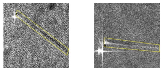
Figure 5.
Polygonal mask annotations of ship wakes labeled using VIA tool.
Concluding this section, it is important to point out that ships have been excluded from labeled polygonal masks. This is crucial to avoid the feature association between wakes and bright ships, which is not always true in practice, i.e., in the case of go-fast vessels [43] or large azimuth offsets [50].
5. Setup and Metrics
In this section, the setup used for implementing architectures introduced in Section 2 is reported, and the evaluation metrics are explained.
5.1. Setup
All the experiments on SSWD are supported by a local machine with the 64-bit Ubuntu 18.04 operating system. The software configuration consisted of a python environment, Detectron2 [51] build on top of PyTorch 1.9.0 framework, CUDA 10.2, cuDNN 8.1.0. The hardware used includes NVIDIA GTX-1060 GPU (6 GB memory) and Intel i5-8600K CPU @3.60 GHz and 16 GB RAM.
All the hyperparameters were kept the same to compare the performance of the detectors. The latter were trained with GPU and finished in 5000 epochs. In the standard way, the weight decay and momentum were set to 0.0001 and 0.9, respectively. The IoU threshold was set to 0.5 when training and validating, while the IoU thresholds for Cascade R-CNN are set to {0.5, 0.6, 0.7}. The optimizer selected was SGD (stochastic gradient descent) with a learning rate of 0.0005. Due to the high dimension of the objects in the dataset, anchor sizes have been raised to {32, 64, 128, 256, 512}, while the anchor scales were left as defaults {0.5, 1, 2}. The parameters related to RPN were left as default for all detectors and are reported in Table 1.

Table 1.
RPN training parameters.
In the end, the details of RetinaNet implementation related to its focal loss are set according to [52], which applied the method for ship detection in SAR images. Relevant parameters are reported in Table 2.
Table 2.
RetinaNet training parameters.
The rest of the hyperparameters were set according to the default values of the baseline implementations.
5.2. Evaluation Metrics
The performance evaluation of object detectors was commonly carried out by normative metrics such as IoU (intersection over union), precision, recall and . In supervised learning, the labeled data was used to estimate the overlap rate, i.e., the correlation between prediction and ground truth. This is measured by IoU, defined as:
where and denote the predicted and ground truth bounding box, respectively. Depending on the threshold set for IoU, a classifier may misjudge background and instances. Thus, it is possible to divide the classification results into four categories: True Positives (TP), True Negatives (TN), False Negatives (FN) and False Positives (FP). TP and TN denote the amount of correctly classified positive and negative samples, respectively. FP and FN denote the number of false alarms and missed positive samples, respectively. Precision and recall are defined as:
In the Cartesian coordinate system, placing the horizontal coordinate on the recall and the vertical precision, the precision-recall curve was obtained. The precision-recall curve shows the trade-off between precision and recall for different IoU thresholds. The (average precision) can be defined as the area under this curve, as shown in Equation (13):
in which P represents precision and r represents recall. When multiple categories are present, the average prompted on all categories is defined as the mean or .
Common dataset evaluation formats are pascal visual object classes (Pascal VOC) [53] and Microsoft Common Objects in Context (MS COCO) [54]. Since MS COCO metrics are abundant and comprehensive, MS COCO evaluation metrics were applied for the evaluation of the proposed dataset. MS COCO has the strict metric of IoU thresholds, such as , and , which is the primary challenge metric. The subscript denotes the calculation under the specified IoU threshold. The calculation was instead an average of ten IoU thresholds distributed from 0.5 to 0.95 with a constant step of 0.05. In terms of the capabilities in multi-scale object detection, MS COCO scale division for object detection [54] groups the instances into three categories, i.e., , and . The small objects () are characterized by bounding box areas below 32 × 32 pixels, while the large objects () have an area above 96 × 96 pixels. The latter metrics are more specific for camera images.
, , have been taken to benchmark the performance of the detectors on SSWD.
6. Results
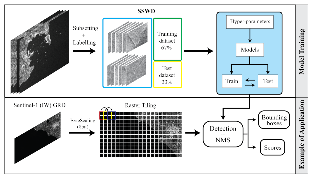
In this section, the architectures introduced in Section 2 were implemented for the DL-based wake detection in order to gain further insight into the evaluation metrics of each architecture. Then, the detection performance of the best-trained model was evaluated on a test scenario in the Gulf of La Spezia, Italy, where ground truth (AIS) was available. A detailed workflow of the proposed methodology is reported in Figure 6. Finally, a further application on X-band products in different polarizations is shown.

Figure 6.
Workflow of the proposed methodology: (top) model training and (bottom) model performance evaluation on a test scenario in the Gulf of La Spezia.
6.1. Results on SSWD
Since there is only one class, problems of class imbalance were not faced. However, the wake detection problem was still intrinsically tricky to solve due to the coherent speckle-noise always present both in the clutter and the wake. As stated above, Faster R-CNN, RetinaNet, Mask R-CNN and Cascade Mask R-CNN have been benchmarked with different backbone combinations. The utilized baselines include both ResNet-50 and ResNet-101 coupled with (a) FPN: use ResNet + FPN (feature pyramid network) with standard conv and FC heads for mask and bounding box predictions; (b) ResNet+C4: use ResNet conv4 backbone with conv5 head; (c) DC5 (Dilated-C5): use a ResNet conv5 backbone with dilations in conv5, and standard conv and FC heads for mask and box prediction, respectively [51].
A transfer-learning procedure is carried out for all the models on SSWD. Both the pre-trained weights of ImageNet and Coco datasets have been tested but, since ImageNet weights have achieved lower results, they have not been reported. As stated above, the fine-tuning has been performed training 5000 epochs with SGD and a learning rate of 0.0005. Our training strategy involves early-stopping of the models with the best (mean average precision) for taking into account both precision and recall. For this purpose, a hook function has been implemented to evaluate the models on the test set every 50 epochs. It is worth noting that since there is only one class, and coincide. A data augmentation strategy (i.e., resizing, shifting, flipping and rotating) is also involved to prevent overfitting. The performance of heavily under-trained weights (∼12 coco epochs) have been evaluated. Table 3 compares model scores on , and . The is equal to in this case because it was not possible to estimate and . This indicates that SSWD are not present as a significant number of small and medium wake instances. Deeper networks involving ResNet-101 have achieved better performance (by mean ) on SSWD. The best backbone combination is ResNet + FPN, followed by slight improvements of ResNet + DC5 against ResNet + C4. In all cases, the under-trained weights have shown lower performance. The best model so far is Cascade Mask R-CNN, which achieved a of . In Figure 7, the training and validation losses are reported over 5000 iterations of the model.
Table 3.
Coco evaluation of the state-of-art object detection models of SSWD.

Figure 7.
Sentinel-1 GRD (IW) image gathered in VV polarization over La Spezia on 18/07/2020 at 17:14 UTC (latitude-longitude coordinates). Product ID: S1A_IW_GRDH_1SDV_20200718T171436_20200718T171501_033512_03_E220_DEFC.
As highlighted in the graph, the validation loss function stabilizes after 1000 iterations, while the training loss continues to decrease.
As is possible to notice, the graph shows the that started climbing steadily, peaking at ∼1500 iterations. The trends of the and validation loss demonstrate that, despite the small dataset, overfitting has been properly handled. Our preliminary results on SSWD regarding SS-ODs show no significant improvements against the Cascade approach. Nonetheless, additional tests are demanded in the future, even combining the two methodologies.
6.2. Results on a Sentinel-1 Product
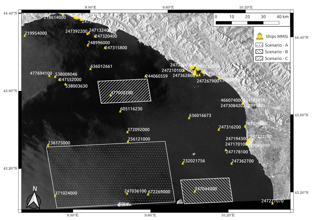
Wake detection is herein discussed for a VV-polarized IW-GRD Sentinel-1 image (Figure 7) gathered over the Gulf of La Spezia, Italy.
The satellite image is completed by AIS data, acquired by the AIS ground station of La Spezia-Castellana (Station #890) at latitude and longitude of 44.07° North and 9.82° East, respectively, and from an altitude above sea level of about 200 m. Figure 7 shows three scenarios selected in different environments and sea-state conditions, Scenario A illustrates the detection over a condition of the rough sea with surface natural films (Figure 8), Scenario B includes an area of quiet sea condition (Figure 9), and Scenario C is characterized by areas of wind-speed change (Figure 10). It is worth detailing that with the nomenclature, surface films including eddies or other surface currents, as used in [12]. In order to analyze the detection performance of the best-trained model, i.e., Cascade Mask R-CNN (ResNet-50 + FPN backbone), it is worth noting that there is a significant difference between a tile and entire Sentinel-1 imagery. Indeed, a raster-tiling and a non-max suppression (NMS) algorithm are required as pre-processing and post-processing steps, respectively, to not lose the receptive field.

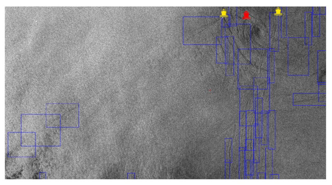
Figure 8.
Detections over Scenario A (Azimuth-Ground Range coordinates). Dark vessel in middle indicated in red.
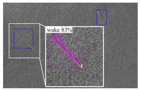
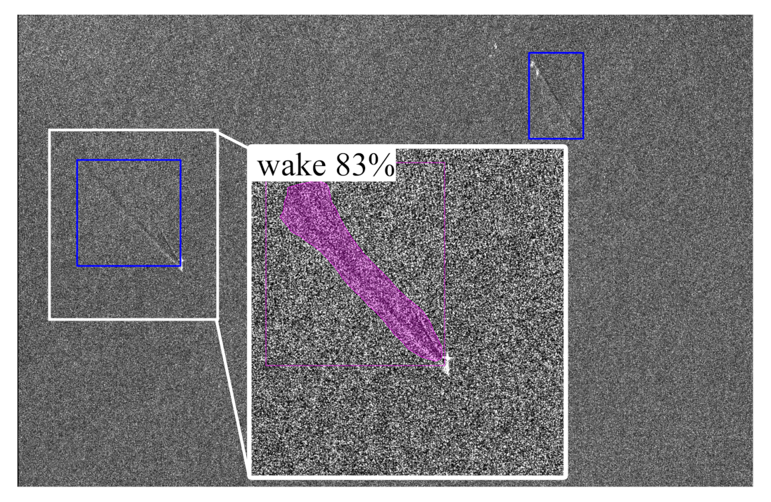
Figure 9.
Detections over Scenario B (Azimuth-Ground Range coordinates).
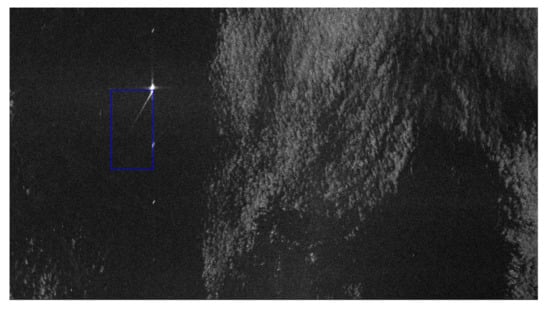
Figure 10.
Detections over Scenario C (Azimuth-Ground Range coordinates).
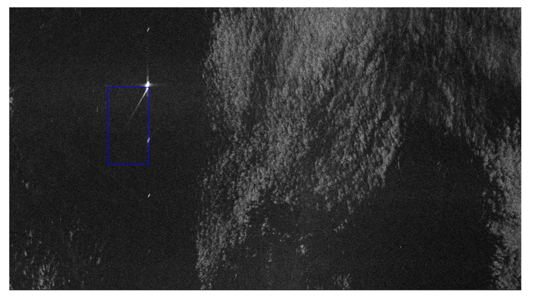
A land-masking and common byte-scaling have been performed using the SNAP (ESA) processing toolbox, using the SRTM 3 sec DEM with an extended shoreline of 10 px. Then, a sliding window of 1000 × 1000 pixels moves with a stride of 500 pixels; despite the usage of a modest hardware, the 4264 tiles obtained are processed in less than 800 s. As seen from Figure 8, in scenario A, two collaborative ships and a dark vessel in the middle are present.
The blue rectangles in Figure 8, Figure 9 and Figure 10 represent the bounding boxes output of Cascade Mask R-CNN after the non-maximum suppression algorithm. As stated above, NMS and raster-tiling are demanded due to the impossibility of performing an end-to-end training with a single GPU. These detections are filtered with a global confidence score threshold of 0.55.
The narrow natural surface films have been imaged as an almost straight feature and, hence, have been interpreted by the algorithm as ship wakes. However, all the wakes have been detected with the commonly assumed confidence score threshold of 0.55. More in detail, the trace of the ship wake on the left has shown an interesting behaviour since it extends for several kilometers: in the section where the contrast is poor, the detector was not able to find the wake, but in a close section the contrast boost led the detection again to be feasible. In a quiet sea condition (scenario B), the detector has shown a remarkable performance able to capture all the wakes with no false alarms. For the sake of highlighting the capability of the algorithm, the binary mask obtained by the segmentation branch of Cascade Mask R-CNN and the confidence score of one of the two detected wakes is also reported. In Scenario C, the wind-speed change has generated a variation of the backscattered energy from the sea, thus, a particular pattern is visible. Still, the detector has been able to handle this situation with no false alarm generated in a bright/dark border and the unique ship wake in the scene is correctly detected.
From a statistical point of view, an error analysis of the detector has been conducted on whole SAR images covering the Gulf of Genoa, Italy. They are Interferometric Wide (IW) swath mode Sentinel-1 C-band images gathered in VV polarization, and correspond to Level-1 Ground Range Detected (GRD) products. All the images are acquired in ascending phase with a ground range and an azimuth spacing of 10 m. The following Table 4, lists the image IDs completed by wind and maritime traffic data, provided by in situ measurements at Genoa and La Spezia stations, respectively. The images are not present in the paper for brevity but are reported in the Supplementary Materials.
Table 4.
List of products under inspection for error analysis.
We denote TP as the true positives, TN, the true negative, and FP, the false negatives. The available data allow us to affirm that when the turbulent wake is clearly focused by SAR, the trained detector provides almost 100% of TP, i.e., all the wakes are detected by the model, 0% of TN, i.e., no wake imaged in the scene is lost, but is very difficult to quantify the FP. This is due to the impossibility of the identification of a ground truth, even with a visual inspection of the SAR image. In some cases, false positives clearly derived from other features over sea, such as natural surface films, but in other cases, mainly when the ship is not imaged, it is not possible to discriminate about the nature of the feature.
6.3. Results on X-Band Products
As domain shifting and transfer learning are a common practice in deep learning, in this section the generalizability reached by the developed and trained detector is assessed. Thus, the detection performances are hereby evaluated on the German TerraSAR-X (TSX) and Italian Cosmo-Skymed (CSK) X-band products. Main characteristics are reported in Table 5, where it is possible to notice that the products are in Azimuth-Slant Range coordinates.
Table 5.
Main characteristics of TerraSAR-X (TSX) and Cosmo-Skymed (CSK) X-band products.
It is worth noting that the algorithm has been trained on C-band images, which, in terms of complexity, offer relatively fewer features compared to X-band SAR imagery. The application of the proposed methodology is motivated showing the robustness of the results against multi-domain unseen data.
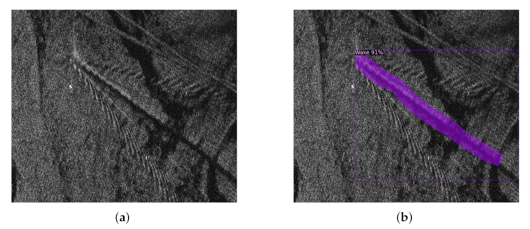
Firstly, the results over TSX data are evaluated. These images hold characteristics similar to sentinel-1 IW products, i.e., the same polarization and same wake characteristics present, but the resolution and wavelength of the signal are different. A subset of the TSX product is reported in (Figure 11a). The product gathered over the Gulf of Naples, Italy, on 9 June 2011 shows two wakes in opposite azimuth directions. The sea state is in a quiet condition and the two turbulent wakes are sharply distinguishable from the sea clutter. The results shown in Figure 11b demonstrate that the detector is able to recognize the presence of two different ship wakes; this is very interesting since the two wakes barely cross in the bottom, which could be prone to lead to a false interpretation as a unique V-shape wake. The confidence scores are still high enough and the contour of the ship wakes are well defined.
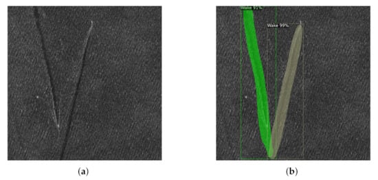
Figure 11.
Subset (2000 × 2000 pixels) of the TSX product (TSX1_SAR_SSC_BTX1_SM_D_SRA_20110609T164931_20110609T164939) gathered in VV polarization over the Gulf of Naples, Italy on 9 June 2011 (Azimuth-Slant Range coordinates). (a) Reference image, (b) Segmentation results.
Finally, results are evaluated on CSK data, which are completely different in terms of sensor, resolution, polarization and different wake characteristics. In Figure 12a, a subset of CSK SLC images in Azimuth-Slant Range coordinates is reported. The image is gathered in HH polarization over the Gulf of Naples, Italy, on 30 June 2008. It contains a ship wake in which the Kelvin wakes generated by the vessel motion are clearly visible. Results shown in Figure 12b confirm the generalization of the proposed methodology. As expected, the segmentation mask well contours the turbulent and narrow-V wakes but does not recognize the kelvin cusps. However, this is quite understandable, since the detector has not been trained to recognize such features, which are not imaged in medium resolution C-band imagery, like Sentinel-1 IW products. It is worth noting that the confidence score is high enough to discriminate the wake from the surrounding surface films, which have not been misjudged by the algorithm.

Figure 12.
Subset (1825 × 1563 pixels) of the CSK product (CSKS1_SCS_B_HI_0B_HH_RA_SF_20080630045711_20080630045718) gathered in HH polarization over the Gulf of Naples, Italy, on 30 June 2008 (Azimuth-Slant Range coordinates). (a) Reference image, (b) Segmentation results.
7. Conclusions
Leveraging the generalization capabilities of DL-based methods, this paper assessed the effectiveness of object detectors for the sake of wake detection in SAR images. With different incident angles of the radar signal, environmental factors, polarization methods, orientations, frequency, ship velocity, ship type, etc., the ship wake greatly changes its appearance. Due to the lack of large datasets in the SAR community, an original dataset of ship wakes (SSWD) has been built, by exploiting the C-band SAR images gathered by Sentinel-1 satellites. Since an assessment about the best DL model for wake detection is not available from the literature, an analysis of metrics has been discussed as limited to the most mature architectures, i.e., the R-CNN family network and RetinaNet. The results provide the first overview of the main properties of DL-based object detectors for wake detection in SAR images. Moreover, the analysis paves the way towards future application of more advanced detectors. In fact, in the last year, Vision Transformer (ViT)-based ODs and SS-ODs are gaining huge attention; since most of these extend the most mature ones, the latter have been assumed as model baselines for these first analyses. The best-trained model, i.e., Cascade Mask R-CNN, is then applied to process a complete Sentinel-1 product. Finally, paving the idea of a domain-agnostic wake detector, the domain generalization performance reached is tested against X-band images coming from TerraSAR-X and Cosmo-Skymed in VV and HH polarization, respectively. The results confirm the performance in terms of detection rate and processing cost of the proposed methodology. Having confirmed that DL can support the achievement of a ship wake detector, future activities will pay attention to the most recent architectures released. Despite the small number of chips contained in SSWD, this study has shown that convergence has occurred. In future, SSWD will be enriched with X-band data, given the importance of the data variety and veracity in the characterization of the ship wake. Another step is the implementation of rotating bounding boxes that may tackle the clutter leakage due to the elongated wake shape. Finally, an ablation study is also required to build a lightweight custom backbone for wake detection purposes, enhancing the object detection performance at a lower computational cost.
The experimental results confirm that the trained and tested detectors cannot be considered enough mature for practical and operational applications. One of the limitations of current development is certainly represented by the limited number of chips of SSWD. However, recollecting ship wake chips by visual inspection requires a significant deal of manpower. Ongoing and future activities are planned to produce a wider database. Another, probably more important, limitation regarding the false alarm rate, especially in rough sea conditions for low-resolution SAR data, the few imaged features could make ship wakes similar to surface films. As a result, this makes it difficult to establish a confidence score threshold to filter out false alarms. To overcome these situations, there is a need for a discrimination step implementing deterministic approaches, e.g., including hydrodynamic laws or multi-polarization measures. One last limitation concerns the way in which detectors were trained and the labeled dataset developed. The results presented in this paper demonstrate that the wake detection problem is very different from the ship detection one. Hence, working with larger chips may represent of valuable approach to catch the spatial variability of the wake features and to enhance the subtle differences distinguishing them from other phenomena affecting SAR imaging over sea and oceans.
Supplementary Materials
Data of the reported results are publicly available on Zenodo at https://zenodo.org/record/5694213#.YY_ksbrSIj4.
Author Contributions
Data curation, R.D.P.; Funding acquisition, M.D.G.; Investigation, A.R.; Methodology, R.D.P. and M.D.G.; Software, R.D.P.; Supervision, M.D.G. and A.R.; Validation, M.D.G.; Writing—original draft, R.D.P. and M.D.G.; Writing—review & editing, A.R. All authors have read and agreed to the published version of the manuscript.
Funding
This research was funded by the University of Naples “Federico II”, in the framework of “PROGRAMMA PER IL FINANZIAMENTO DELLA RICERCA DI ATENEO”—Project: A wake Revelation system for GO-fast vessels (ARGO).
Institutional Review Board Statement
Not applicable.
Informed Consent Statement
Not applicable.
Data Availability Statement
Date of the reported results are on Supplementary materials.
Acknowledgments
This work is based upon information provided by the NATO Science & Technology Organization Centre for Maritime Research and Experimentation (STO-CMRE) www.cmre.nato.int TerraSAR-X data used in this paper were made available by DLR within the first TanDEM-X Announcement of Opportunity (Proposal OTHER0456). The analyses were also carried out using CSK products from ASI (Italian Space Agency) delivered under an ASI license to use in the framework of COSMO-SkyMed Open Call for Science, proposal reference code 0015/8/194/115.
Conflicts of Interest
The authors declare no conflict of interest.
References
- Balkin, R. The International Maritime Organization and Maritime Security. Tul. Mar. LJ 2006, 30, 1. [Google Scholar]
- Tetreault, B.J. Use of the Automatic Identification System (AIS) for Maritime Domain wareness (MDA). In Proceedings of the Oceans 2005 Mts/IEEE, Washington, DC, USA, 17–23 September 2005; pp. 1590–1594. [Google Scholar]
- Iceye. Dark Vessel Detection for Maritime Security with SAR Data. 2021. Available online: https://www.iceye.com/use-cases/security/dark-vessel-detection-for-maritime-security (accessed on 19 May 2021).
- exactEarth. exactEarth | AIS Vessel Tracking | Maritime Ship Monitoring | Home. 2021. Available online: https://www.exactearth.com/ (accessed on 19 May 2021).
- Graziano, M.D.; Renga, A.; Moccia, A. Integration of Automatic Identification System (AIS) Data and Single-Channel Synthetic Aperture Radar (SAR) Images by SAR-Based Ship Velocity Estimation for Maritime Situational Awareness. Remote Sens. 2019, 11, 2196. [Google Scholar] [CrossRef] [Green Version]
- Li, J.; Qu, C.; Shao, J. Ship Detection in SAR Images Based on an Improved Faster R-CNN. 2017 SAR in Big Data Era: Models, Methods and Applications (BIGSARDATA); IEEE: Piscataway, NJ, USA, 2017; pp. 1–6. [Google Scholar]
- Pei, J.; Huang, Y.; Huo, W.; Zhang, Y.; Yang, J.; Yeo, T.S. SAR automatic target recognition based on multiview deep learning framework. IEEE Trans. Geosci. Remote Sens. 2017, 56, 2196–2210. [Google Scholar] [CrossRef]
- Zhao, P.; Liu, K.; Zou, H.; Zhen, X. Multi-stream convolutional neural network for SAR automatic target recognition. Remote Sens. 2018, 10, 1473. [Google Scholar] [CrossRef] [Green Version]
- Potin, P.; Rosich, B.; Miranda, N.; Grimont, P. Sentinel-1a/-1b mission status. In Proceedings of the 12th European Conference on Synthetic Aperture Radar— VDE (EUSAR 2018), Berlin, Germany, 2–6 June 2018; pp. 1–5. [Google Scholar]
- Karakuş, O.; Achim, A. On Solving SAR Imaging Inverse Problems Using Nonconvex Regularization with a Cauchy-Based Penalty. IEEE Trans. Geosci. Remote Sens. 2020, 59, 5828–5840. [Google Scholar] [CrossRef]
- Graziano, M.D.; D Errico, M.; Rufino, G. Ship heading and velocity analysis by wake detection in SAR images. Acta Astronaut. 2016, 128, 72–82. [Google Scholar] [CrossRef]
- Liu, P.; Zhao, C.; Li, X.; He, M.; Pichel, W. Identification of ocean oil spills in SAR imagery based on fuzzy logic algorithm. Int. J. Remote Sens. 2010, 31, 4819–4833. [Google Scholar] [CrossRef]
- Gu, F.; Zhang, H.; Wang, C. A two-component deep learning network for SAR image denoising. IEEE Access 2020, 8, 17792–17803. [Google Scholar] [CrossRef]
- Schmitt, M.; Hughes, L.H.; Zhu, X.X. The SEN1-2 dataset for deep learning in SAR-optical data fusion. arXiv 2018, arXiv:1807.01569. [Google Scholar] [CrossRef] [Green Version]
- Cha, M.; Majumdar, A.; Kung, H.; Barber, J. Improving SAR automatic target recognition using simulated images under deep residual refinements. In Proceedings of the 2018 IEEE International Conference on Acoustics, Speech and Signal Processing (ICASSP), Calgary, AB, Canada, 15–20 April 2018; pp. 2606–2610. [Google Scholar]
- Wang, Y.; Wang, C.; Zhang, H.; Dong, Y.; Wei, S. A SAR dataset of ship detection for deep learning under complex backgrounds. Remote Sens. 2019, 11, 765. [Google Scholar] [CrossRef] [Green Version]
- Chang, Y.L.; Anagaw, A.; Chang, L.; Wang, Y.C.; Hsiao, C.Y.; Lee, W.H. Ship detection based on YOLOv2 for SAR imagery. Remote Sens. 2019, 11, 786. [Google Scholar] [CrossRef] [Green Version]
- Kang, K.m.; Kim, D.j. Ship velocity estimation from ship wakes detected using convolutional neural networks. IEEE J. Sel. Top. Appl. Earth Obs. Remote Sens. 2019, 12, 4379–4388. [Google Scholar] [CrossRef]
- Ren, S.; He, K.; Girshick, R.; Sun, J. Faster R-CNN: Towards Real-Time Object Detection with Region Proposal Networks. arXiv 2015, arXiv:1506.01497. [Google Scholar] [CrossRef] [PubMed] [Green Version]
- Krizhevsky, A.; Sutskever, I.; Hinton, G.E. Imagenet classification with deep convolutional neural networks. Adv. Neural Inf. Process. Syst. 2012, 25, 1097–1105. [Google Scholar] [CrossRef]
- Zeiler, M.D.; Fergus, R. Visualizing and understanding convolutional networks. In European Conference on Computer Vision; Springer: Zurich, Switzerland, 2014; pp. 818–833. [Google Scholar]
- Simonyan, K.; Zisserman, A. Very Deep Convolutional Networks for Large-Scale Image Recognition. arXiv 2014, arXiv:1409.1556. [Google Scholar]
- Szegedy, C.; Liu, W.; Jia, Y.; Sermanet, P.; Reed, S.; Anguelov, D.; Erhan, D.; Vanhoucke, V.; Rabinovich, A. Going deeper with convolutions. In Proceedings of the IEEE Conference on Computer Vision and Pattern Recognition, Boston, MA, USA, 7–12 June 2015; pp. 1–9. [Google Scholar]
- He, K.; Zhang, X.; Ren, S.; Sun, J. Deep Residual Learning for Image Recognition. 2015. Available online: http://xxx.lanl.gov/abs/1512.03385 (accessed on 19 May 2021).
- Girshick, R.; Donahue, J.; Darrell, T.; Malik, J. Rich feature hierarchies for accurate object detection and semantic segmentation. arXiv 2013, arXiv:1311.2524. [Google Scholar]
- Hoiem, D.; Divvala, S.K.; Hays, J.H. Pascal VOC 2008 Challenge. World Literature Today. 2009. Available online: http://host.robots.ox.ac.uk/pascal/VOC/voc2008/index.html (accessed on 19 May 2021).
- Liu, Y.C.; Ma, C.Y.; He, Z.; Kuo, C.W.; Chen, K.; Zhang, P.; Wu, B.; Kira, Z.; Vajda, P. Unbiased teacher for semi-supervised object detection. arXiv 2021, arXiv:2102.09480. [Google Scholar]
- Xu, M.; Zhang, Z.; Hu, H.; Wang, J.; Wang, L.; Wei, F.; Bai, X.; Liu, Z. End-to-End Semi-Supervised Object Detection with Soft Teacher. arXiv 2021, arXiv:2106.09018. [Google Scholar]
- Law, H.; Deng, J. Cornernet: Detecting Objects as Paired Keypoints. In Proceedings of the European Conference on Computer Vision (ECCV), Munich, Germany, 8–14 September 2018; pp. 734–750. [Google Scholar]
- Zhou, X.; Wang, D.; Krähenbühl, P. Objects as points. arXiv 2019, arXiv:1904.07850. [Google Scholar]
- Tian, Z.; Shen, C.; Chen, H.; He, T. Fcos: Fully convolutional one-stage object detection. In Proceedings of the IEEE/CVF International Conference on Computer Vision, Seoul, Korea, 27 October–2 November 2019; pp. 9627–9636. [Google Scholar]
- Beal, J.; Kim, E.; Tzeng, E.; Park, D.H.; Zhai, A.; Kislyuk, D. Toward transformer-based object detection. arXiv 2020, arXiv:2012.09958. [Google Scholar]
- Carion, N.; Massa, F.; Synnaeve, G.; Usunier, N.; Kirillov, A.; Zagoruyko, S. End-to-end object detection with transformers. In European Conference on Computer Vision; Springer: Zurich, Switzerland, 2020; pp. 213–229. [Google Scholar]
- Khan, S.; Naseer, M.; Hayat, M.; Zamir, S.W.; Khan, F.S.; Shah, M. Transformers in vision: A survey. arXiv 2021, arXiv:2101.01169. [Google Scholar]
- Memisevic, R.; Zach, C.; Pollefeys, M.; Hinton, G.E. Gated softmax classification. Adv. Neural Inf. Process. Syst. 2010, 23, 1603–1611. [Google Scholar]
- He, K.; Gkioxari, G.; Dollár, P.; Girshick, R. Mask R-CNN. 2018. Available online: http://xxx.lanl.gov/abs/1703.06870 (accessed on 19 May 2021).
- Han, J.; Moraga, C. The influence of the sigmoid function parameters on the speed of backpropagation learning. In International Workshop on Artificial Neural Networks; Springer: Torreomolinos, Spain, 1995; pp. 195–201. [Google Scholar]
- Cai, Z.; Vasconcelos, N. Cascade R-CNN: High Quality Object Detection and Instance Segmentation. 2019. Available online: http://xxx.lanl.gov/abs/1906.09756 (accessed on 19 May 2021).
- Lin, T.Y.; Goyal, P.; Girshick, R.; He, K.; Dollár, P. Focal loss for dense object detection. In Proceedings of the IEEE International Conference on Computer Vision, Venice, Italy, 22–29 October 2017; pp. 2980–2988. [Google Scholar]
- Lin, T.Y.; Dollár, P.; Girshick, R.; He, K.; Hariharan, B.; Belongie, S. Feature Pyramid Networks for Object Detection. 2016. Available online: http://xxx.lanl.gov/abs/1612.03144 (accessed on 19 May 2021).
- Pichel, W.G.; Clemente-colón, P.; Wackerman, C.C.; Friedman, K.S. Ship and Wake Detection. In SAR Marine Users Manual; NOAA: Washington, DC, USA, 2004; Available online: https://www.sarusersmanual.com/ (accessed on 19 May 2021).
- Darmon, A.; Benzaquen, M.; Raphaël, E. Kelvin wake pattern at large Froude numbers. J. Fluid Mech. 2014, 738, R3. [Google Scholar] [CrossRef] [Green Version]
- Tunaley, J.K. Wakes from Go-Fast and Small Planing Boats; London Research and Development Corporation: Ottawa, ON, Canada, 2014. [Google Scholar]
- Tings, B.; Velotto, D. Comparison of ship wake detectability on C-band and X-band SAR. Int. J. Remote Sens. 2018, 39, 4451–4468. [Google Scholar] [CrossRef] [Green Version]
- Lyden, J.D.; Hammond, R.R.; Lyzenga, D.R.; Shuchman, R.A. Synthetic aperture radar imaging of surface ship wakes. J. Geophys. Res. Ocean. 1988, 93, 12293–12303. [Google Scholar] [CrossRef]
- Panico, A.; Graziano, M.; Renga, A. SAR-Based Vessel Velocity Estimation from Partially Imaged Kelvin Pattern. IEEE Geosci. Remote Sens. Lett. 2017, 14, 2067–2071. [Google Scholar] [CrossRef]
- Hennings, I.; Romeiser, R.; Alpers, W.; Viola, A. Radar imaging of Kelvin arms of ship wakes. Int. J. Remote Sens. 1999, 20, 2519–2543. [Google Scholar] [CrossRef]
- Graziano, M.D.; Grasso, M.; D’ Errico, M. Performance Analysis of Ship Wake Detection on Sentinel-1 SAR Images. Remote Sens. 2017, 9, 1107. [Google Scholar] [CrossRef] [Green Version]
- Dutta, A.; Zisserman, A. The VIA annotation software for images, audio and video. In Proceedings of the 27th ACM International Conference on Multimedia, Nice, France, 21–25 October 2019; pp. 2276–2279. [Google Scholar]
- Ouchi, K. On the multilook images of moving targets by synthetic aperture radars. IEEE Trans. Antennas Propag. 1985, 33, 823–827. [Google Scholar] [CrossRef]
- Wu, Y.; Kirillov, A.; Massa, F.; Lo, W.Y.; Girshick, R. Detectron2. 2019. Available online: https://github.com/facebookresearch/detectron2 (accessed on 19 May 2019).
- Wei, S.; Zeng, X.; Qu, Q.; Wang, M.; Su, H.; Shi, J. HRSID: A High-Resolution SAR Images Dataset for Ship Detection and Instance Segmentation. IEEE Access 2020, 8, 120234–120254. [Google Scholar] [CrossRef]
- Everingham, M.; Van Gool, L.; Williams, C.K.; Winn, J.; Zisserman, A. The pascal visual object classes (voc) challenge. Int. J. Comput. Vis. 2010, 88, 303–338. [Google Scholar] [CrossRef] [Green Version]
- Lin, T.Y.; Maire, M.; Belongie, S.; Hays, J.; Perona, P.; Ramanan, D.; Dollár, P.; Zitnick, C.L. Microsoft coco: Common objects in context. In European Conference on Computer Vision; Springer: Zurich, Switzerland, 2014; pp. 740–755. [Google Scholar]


Publisher’s Note: MDPI stays neutral with regard to jurisdictional claims in published maps and institutional affiliations. |
© 2021 by the authors. Licensee MDPI, Basel, Switzerland. This article is an open access article distributed under the terms and conditions of the Creative Commons Attribution (CC BY) license (https://creativecommons.org/licenses/by/4.0/).