Validation of Sentinel-2, MODIS, CGLS, SAF, GLASS and C3S Leaf Area Index Products in Maize Crops

Abstract

We proposed a direct approach to validate hectometric and kilometric resolution leaf area index (LAI) products that involved the scaling up of field-measured LAI via the validation and recalibration of the decametric Sentinel-2 LAI product. We applied it over a test study area of maize crops in northern China using continuous field measurements of LAINet along the year 2019. Sentinel-2 LAI showed an overall accuracy of 0.67 in terms of Root Mean Square Error (RMSE) and it was used, after recalibration, as a benchmark to validate six coarse resolution LAI products: MODIS, Copernicus Global Land Service 1 km Version 2 (called GEOV2) and 300 m (GEOV3), Satellite Application Facility EUMETSAT Polar System (SAF EPS) 1.1 km, Global LAnd Surface Satellite (GLASS) 500 m and Copernicus Climate Change Service (C3S) 1 km V2. GEOV2, GEOV3 and MODIS showed a good agreement with reference LAI in terms of magnitude (RMSE ≤ 0.29) and phenology. SAF EPS (RMSE = 0.68) and C3S V2 (RMSE = 0.41), on the opposite, systematically underestimated high LAI values and showed systematic differences for phenological metrics: a delay of 6 days (d), 20 d and 24 d for the start, peak and the end of growing season, respectively, for SAF EPS and an advance of −4 d, −6 d and −6 d for C3S.

1. Introduction

Leaf area index (LAI), defined as half the total leaf area per unit of ground surface area [1], is a critical variable in land surface processes such as photosynthesis, respiration, and precipitation interception [2]. The Global Climate Observing System (GCOS) identified LAI as one of the essential climate variables accessible from remote sensing observations [3]. Over the last decade, a broad variety of LAI retrieval methods has been proposed and, as described in the literature, they can be grouped in four categories [4]: parametric regression, nonparametric regression, physically based and hybrid methods. Regression methods define statistical relationships between optical remote sensing observations and LAI. A wide variety of statistical approaches mainly based on vegetation indices have been proposed in the literature (e.g., [5]). The physical methods are based on the inversion of canopy radiative transfer models. Among the inversion techniques, the look up tables (LUTs) are widely used in operational algorithms to process large amounts of remote sensing data due to its ability to speed up the inversion process [6]. Hybrid methods combine physical models with the computational efficiency of non-parametric regression methods [6,7]. Machine learning techniques including Neural Networks (NNs) and Gaussian Process Regression (GPR) are widely used. The NNs require less formal statistical training and can implicitly detect complex nonlinear relationships between dependent and independent variables. The GPR allows handling the model selection issue within a Bayesian framework automatically, which offers the potential advantage of avoiding the traditional empirical and tricky tuning of the free parameters of the model [7]. There are already a wide range of existing remote sensing LAI products with different spatial and temporal resolutions based on above algorithms, including MODerate resolution Imaging Spectroradiometer (MODIS, 500 m, 4-day) [8], Copernicus Global Land Service (CGLS) VEGETATION and PROBA-V bioGEOphysical product Version 2 (GEOV2, 1 km, 10-day) [9], CGLS PROBA-V bioGEOphysical product Version 3 (GEOV3, 300 m, 10-day) [10], Satellite Application Facility EUMETSAT Polar System (SAF EPS, 1.1 km, 10-day) [11], Global LAnd Surface Satellite (GLASS, 500 m, 8-day) [12] and Copernicus Climate Change Service (C3S) PROBA-V product Version 2 (C3S V2, 1 km, 10-day) [13] products. Scientific validation is critical to understand their accuracy in order to quantitatively characterize uncertainties embedded in LAI products and acquire key feedback for algorithm improvement [14].

The Land Product Validation (LPV) subgroup of the Committee Earth Observing Satellites’ Working Group on Calibration and Validation (CEOS WGCV) proposed a direct approach for validating coarse resolution LAI products based on the comparison with ground-based reference maps [15]. The field-measured LAI cannot be directly used as a reference for the validation of satellite products due to the scale differences and surface heterogeneity issues [16]. To alleviate the footprint differences, the field-measured LAI acquired within decametric elementary sampling units (ESUs) are scaled up via high-resolution data [2,17] and empirical calibration functions. Then, the high-resolution ground-based maps are aggregated to match the spatial resolution of the LAI products and used as a reference for their validation [15]. A series of studies on the validation of global LAI products have been carried out based on this upscaling validation strategy [18,19].

Up to now, the majority of validation activities have been conducted for hectometric and kilometric (300–1000 m) coarse resolution products [20,21]. Only few studies have focused on the validation of decametric LAI products [19,22,23]. In addition, the existing validation activities only have focused on a single scale although the LAI products across different scales may be inconsistent [24]. Therefore, a joint validation exercise of multi-resolution LAI products is imperative to elucidate scale effects on different LAI products. The validation of temporal performance is also extremely lacking, especially for multi-resolution LAI products. Multi-temporal validation activities are key since the temporal consistency of satellite time series and their accuracy to monitor actual vegetation phenology is mandatory for a successful application of LAI products in land surface and climate models, and in environmental and global change research [25].

Accurate and representative field measurements are key for the validation of LAI satellite products. The direct LAI measurements using litter fall traps and destructive harvest techniques are accurate but time and labor consuming [26]. Currently, the most commonly used LAI field measurements rely on indirect methods based on the light transmittance through the canopy as measured with optical instruments, such as Digital Hemispherical Photographs [27], Tracing Radiation and Architecture of Canopies [28] and LAI-2000 Plant Canopy Analyzer [29], among others [30]. However, temporally continuous field measurements over large spatial areas cannot be easily obtained using these traditional optical instruments. Wireless sensor networks (WSN) are a new type of information acquisition technology, capable of providing novel opportunities to achieve continuous LAI measurement over spatially distributed samples [31,32]. Among the existing WSN-based LAI observation systems, LAINet has been widely used in LAI validation activities [33,34,35].

The goal of the study was to simultaneously validate multiple decametric, hectometric and kilometric LAI products derived from the sensors Sentinel-2, MODIS, PROBA-V and AVHRR. We proposed a direct approach to validate coarse resolution LAI products that involved the scaling up of field-measured LAI via the validation and recalibration of the decametric resolution Sentinel-2 LAI product. It is based on the use of temporally continuous LAINet measurements and the recalibration of Sentinel-2 LAI product, and it may constitute an alternative to the standard CEOS LPV upscaling validation strategy. Maize is widely cultivated all over the world, and the annual output ranks first in cereal production [36]. The study was conducted over maize croplands in northwestern China. Section 2 briefly describes the study area, field measurements and the multi-resolution satellite LAI products. Section 3 describes the upscaling validation method. Section 4 displays and discusses the uncertainty of field measurements, the performance of the proposed up-scaling approach and the validation results of multi-scale LAI products. Finally, Section 5 provides the main conclusions.

2. Study Area and Data

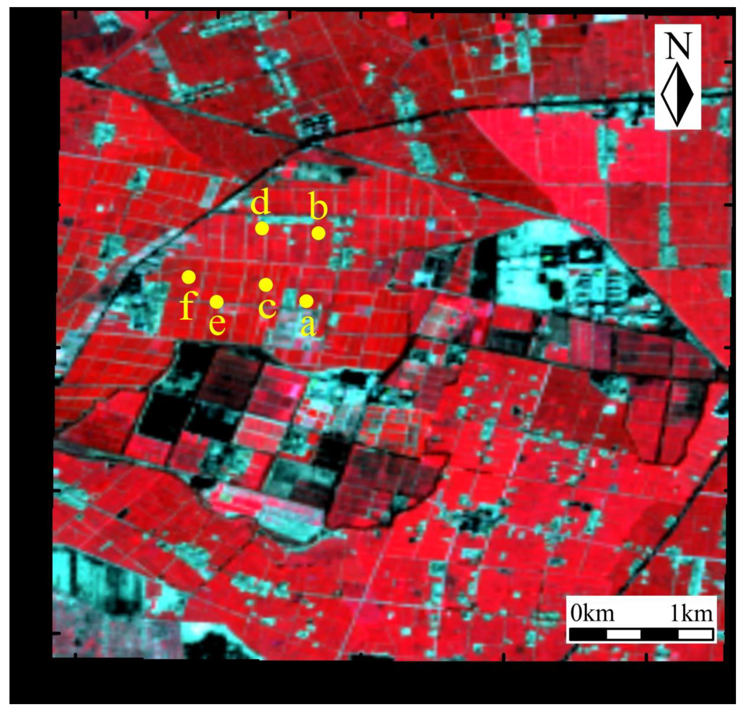
2.1. Study Area and Field Measurements

This study was conducted in a 5 km × 5 km maize cropland region (centered at 38°51′N, 100°22′E) near Zhangye city, China (Figure 1). Zhangye is the largest maize breeding area in China, with an annual output of 450 million kilograms of maize seeds, accounting for more than 50% of China’s annual consumption. The study area is flat with an average altitude of 1579 m. The study is characterized by a temperate continental climate. The total annual precipitation is 129 mm and annual average temperature is 6 °C. Croplands is the dominant land cover type and maize is the primary crop species. The growth stage of maize in our study area can be split into five stages: (1) sowing stage after late April; (2) seedling stage from May until late June; (3) heading stage from late June to late July; (4) mature stage from August to late September; and (5) harvesting stage after late September. Figure 1 shows the location of the study area and the spatial distribution of six ESUs.

A LAINet system was installed in our study area to provide temporally continuous LAI measurements along the year 2019. The effective LAI values are derived from the canopy gap fraction [37], calculated from the ratio between the below-canopy transmitted radiation and above-canopy total downward solar radiation [37]. The two radiation fluxes are automatically measured from above and below nodes, respectively, and the readings are collected by a central node and finally transferred to a remote data server through a general packet radio service network. The above and below nodes have the same hardware configuration and software functions except for their different shapes and the number of integrated optical sensors. In this study, four below nodes per ESU were deployed to measure below-canopy transmitted radiation at the ESU scale with a size of 30 m × 30 m. Only one above node per ESU was deployed, assuming the homogeneity of the incoming solar radiation above the canopy. After the sampling design, the optical sensors are calibrated to ensure that all sensor readings are the same under the same downward radiation conditions, which is a guarantee of the correct measurement of canopy transmittance and the basis to calculate LAI. For details regarding the LAINet, please refer to Qu et al. [38]. The implementation period of the LAINet in our study spanned from 1 June to 20 September 2019 (i.e., from day of year (DOY) 152 to 263), nearly covering the entire growing season of maize crop.

2.2. Leaf Area Index Satellite Products

Seven LAI products, i.e., Sentinel-2, MODIS, GEOV2, GEOV3, EPS, GLASS and C3S, were validated in this study. All the LAI products covering the whole growing cycle of maize were validated and the poor-quality data were discarded by consulting quality control layers.

Table 1. Multi-resolution LAI products investigated in the study.

LAI Products	Algorithm	Sensor/ Platform	Spatial Resolution	Temporal Resolution	Reference
Sentinel-2	Neural networks	MSI/ Sentinel-2	20 m	5-day	[39]
MODIS V6	Look-up-table	MODIS/ Terra + Aqua	500 m	4-day	[40]
GEOV2: CGLS 1 km V2.0	Neural networks	PROBA-V/ PROBA-V	1 km	10-day	[41]
GEOV3: CGLS 300 m	Neural networks	PROBA-V/ PROBA-V	300 m	10-day	[10,42]
SAF EPS V1.0	Gaussian process regression	AVHRR/ MetOp	1.1 km	10-day	[11]
GLASS V5	Neural networks	MODIS/ Terra	500 m	8-day	[32]
C3S V2	Look-up-table	PROBA-V/ PROBA-V	1 km	10-day	[13]

lists the multi-resolution LAI products validated in this study.

2.2.1. Sentinel-2 LAI

The Sentinel-2 mission consists of a constellation of two satellites: Sentinel-2A and Sentinel-2B which both carry the Multi Spectral Instrument (MSI). The two satellites allow a repeat cycle of 5 days and take images in 13 spectral bands at spatial resolutions of 10 m (blue, green, red, near infrared (NIR) bands), 20 m (three vegetation red edge bands, narrow NIR band, two short wave infrared (SWIR) bands) and 60 m (coastal aerosol, water vapour, SWIR-Cirrus bands). We collected all the available Sentinel-2 L1C (Top-of-Atmosphere, TOA, reflectance) data (22 scenes) from 1 April 2019 to 31 October 2019 from the Sentinel data access hub (Available online: https://scihub.copernicus.eu/(accessed on 4 November 2021)). Only images without cloud cover in the study area were selected. The L1C data were corrected atmospherically to L2A data using the Sen2Cor processor (Version 2.8) [43]. Then the Sentinel-2 L2A 10 m spatial resolution bands were resampled to 20 m spatial resolution using the nearest neighbor method. The Simplified Level 2 Product Prototype Processor (SL2P) algorithm [39] integrated in the Sentinel Application Platform (SNAP) was applied to derive Sentinel-2 LAI from Sentinel-2 L2A images. SL2P is a hybrid retrieval algorithm based on back-propagation Neural Networks (NNs) trained over a globally representative set of simulations from PROSAIL model [44]. The L2A reflectances at nine spectral bands (green, red, red edge, narrow NIR and two SWIR bands) were used as input of the NNs. In addition to effective LAI, the SL2P algorithm was here used to estimate the canopy chlorophyll content (cf. Section 4.2).

2.2.2. MODIS LAI

The MODIS collection 6 (C6) LAI product (MCD15A3H) with 500 m spatial resolution is retrieved from combined Terra MODIS and Aqua MODIS every 4 days [40]. We used only the images with good quality (main algorithm with or without saturation), i.e., bit 0 of the quality control layer equals to 0. The main algorithm generating MODIS LAI product is based on a three-dimensional radiative transfer model that is used to generate look-up-tables (LUTs) [45]. The algorithm only uses the red and NIR daily surface reflectance data (MOD09GA, 500 m) as input data because of high uncertainties in other bands [46]. The biome map is another important input, in which global vegetation is classified into eight biomes with different canopy and soil patterns [8,47]. For the observed bi-directional reflectance factors in the red and NIR bands at a specific set of solar and view zenith angles, the algorithm finds the best LAI estimate from biome-specific LUTs. Compositing is done by selecting the daily retrieved value corresponding to maximum LAI over the 4-day compositing period.

2.2.3. GEOV2 LAI

The CGLS 1 km V2.0, here called GEOV2, LAI product derived from SPOT/VEGETATION (for the period from 1999 to May 2014) and PROBA-V (from May 2014 to present) observations is produced globally at 10 days temporal resolution under lat–lon projection at 1/112° spatial resolution [9]. The GEOV2 LAI product capitalizes on existing CYCLOPES V3.1 [48] and MODIS Collection 5 [45] products and the use of NNs. The inputs of the NNs are daily top of the canopy (TOC) reflectances in the red, NIR and SWIR spectral bands and the associated view and sun geometry. The daily LAI outputs of NNs are then filtered, smoothed and gap filled using dedicated temporal compositing techniques to ensure consistency and continuity of the LAI time course every 10 days [9]. The GEOV2 LAI product uses a climatological approach to fill missing data [49].

2.2.4. GEOV3 LAI

The CGLS 300 m, here called GEOV3, LAI product is derived from PROBA-V observations with a 10-day temporal resolution and 300 m spatial resolution [10,42]. GEOV3 algorithm is a simplification and an adaptation of GEOV2 product near real time algorithm [50]. Similar to GEOV2, GEOV3 is based on the use of NNs trained with the fusion of the MODIS C5 and CYCLOPES V3.1 products. NNs are used to provide daily LAI estimates from daily synthesis of PROBA-V reflectances in the blue, red and NIR bands and the view-sun geometry. As for GEOV2, the daily estimates of LAI issued from the NNs are also smoothed and temporally composited at 10-day step to generate the final GEOV3 products. The main difference between the GEOV2 and GEOV3 algorithms is that no climatology is used in GEOV3 methodology to fill missing data [51].

2.2.5. EPS LAI

The SAF EPS LAI product is generated on a 10-day basis at the spatial resolution of 1.1 km from the Advanced Very High Resolution Radiometer (AVHRR) sensor onboard the Meteorological–Operational (MetOp) satellite constellation. LAI is estimated with a hybrid retrieval approach that relies on the PROSAIL model inversion with a Gaussian Process Regression (GPR) [4]. The PROSAIL radiative transfer model is first applied in direct mode to build a representative database containing three short-wave channels (0.6 µm, 0.8 µm, 1.6 µm) and LAI for a broad set of canopy parameterizations and observation conditions. The generated simulations are then used to train a GPR. Finally, after calibration, the GPR is applied to estimate effective LAI using as inputs the atmospherically corrected cloud-cleared 10-day nadir normalized spectral reflectance factor in the red, NIR and Mid-infrared (MIR) EPS bands.

2.2.6. GLASS LAI

The GLASS LAI product at 8-day and 500 m spatial resolution is produced from MOD09A1 8-day surface reflectance data [32]. The GLASS LAI is estimated using a general regression neural network (GRNN). Firstly, the effective CYCLOPES LAI is converted to true LAI using the clumping index [52]. The true LAI is then combined with the MODIS LAI through a weighted linear combination according to their uncertainties determined from the ground-measured true LAI. The original MODIS reflectance data (MOD09A1) are reprocessed to remove cloud contaminated pixels and fill the missing data to obtain continuous and smooth reflectances using the algorithm proposed by Tang et al. [53]. GRNN is trained using the combined LAI and the reprocessed MODIS reflectance data for each biome type over the BELMANIP sites [54]. Finally, the trained GRNN is applied to retrieve LAI from the yearly MOD09A1 surface reflectance product.

2.2.7. C3S V2 LAI

The 1 km C3S V2 LAI product is derived from PROBA-V observations with a 10-day temporal resolution, based on a 31-day observation window with asymmetric weights [13]. The Two-stream Inversion Package (TIP), which relates Bi-Hemispheric Reflectances to various canopy parameters, is applied to visible and NIR broadband albedos to retrieve the LAI. TIP is based on the Two-stream Model developed by Pinty et al. [55], which implements the two-stream approximation of radiative transfer for a homogeneous canopy. The TIP algorithm provides effective LAI. For efficient processing, the retrievals are taken from LUTs, generated with the TIP model [13].

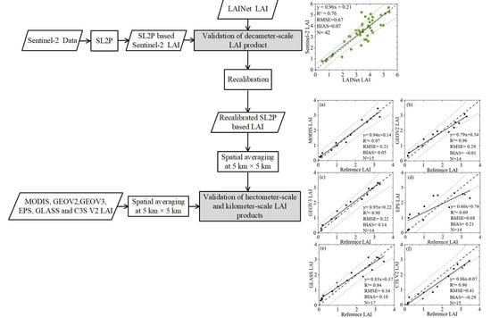
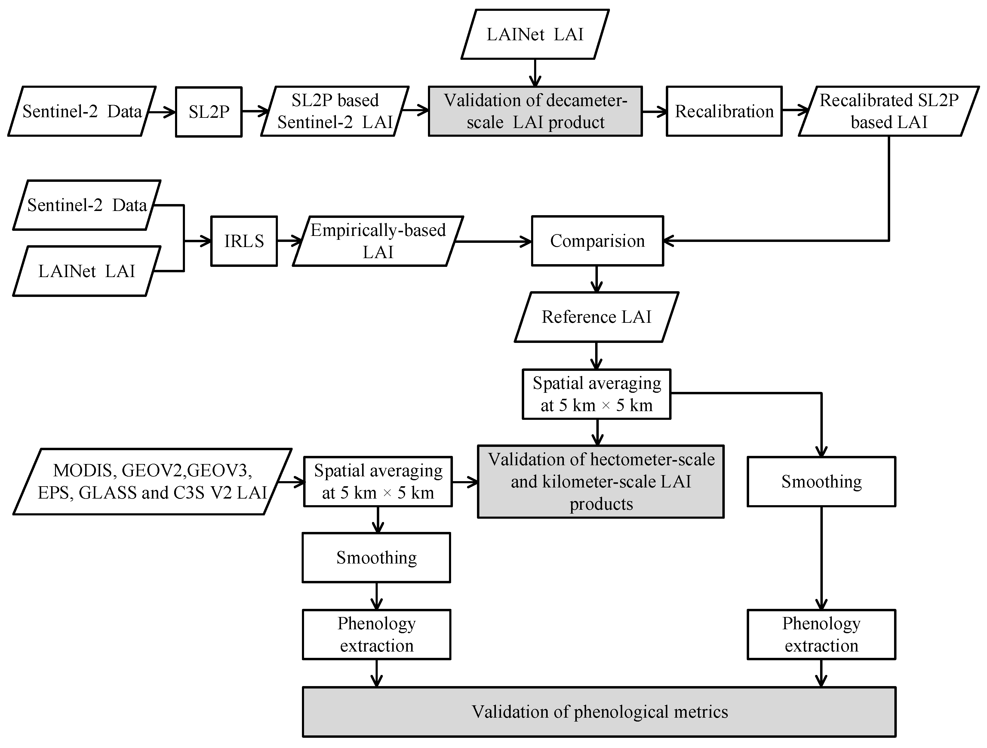
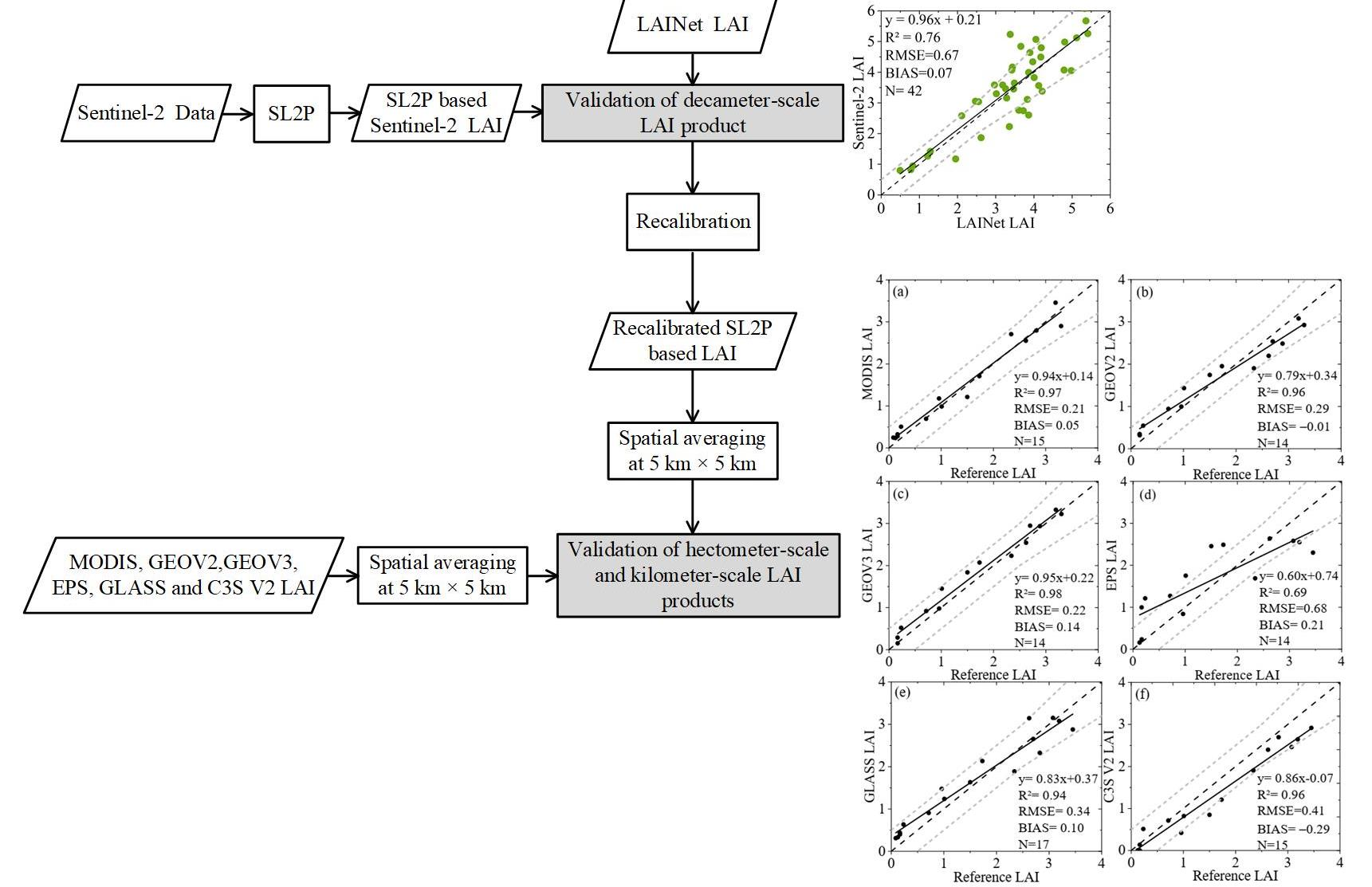
3. Validation Methodology

The validation approach has three main steps (Figure 2): (1) Validation of the SL2P-based Sentinel-2 LAI product and generation of reference LAI maps after recalibration with field measurements; (2) Validation of the hectometric and kilometric MODIS, GEOV2, GEOV3, EPS and GLASS and C3S LAI products; and (3) Validation of the phenological metrics derived from time series of LAI.

3.1. Validation of the Decametric LAI Product and Reference LAIs

The SL2P-based Sentinel-2 LAI product was first validated. Then, two strategies for the generation of reference LAI were compared: (1) recalibrating the SL2P-based Sentinel-2 LAI product with a linear regression against the LAINet LAI, and (2) generating reference LAI through directly up-scaling the LAINet measurements with an empirical transfer function applied to Sentinel-2 reflectances. Results derived from the above two strategies were referred to as recalibrated SL2P-based and empirically based LAIs, respectively. Finally, the best performant LAI, assessed with k-fold cross-validation, was adopted as the reference LAI to validate the hectometric and kilometric LAI products.

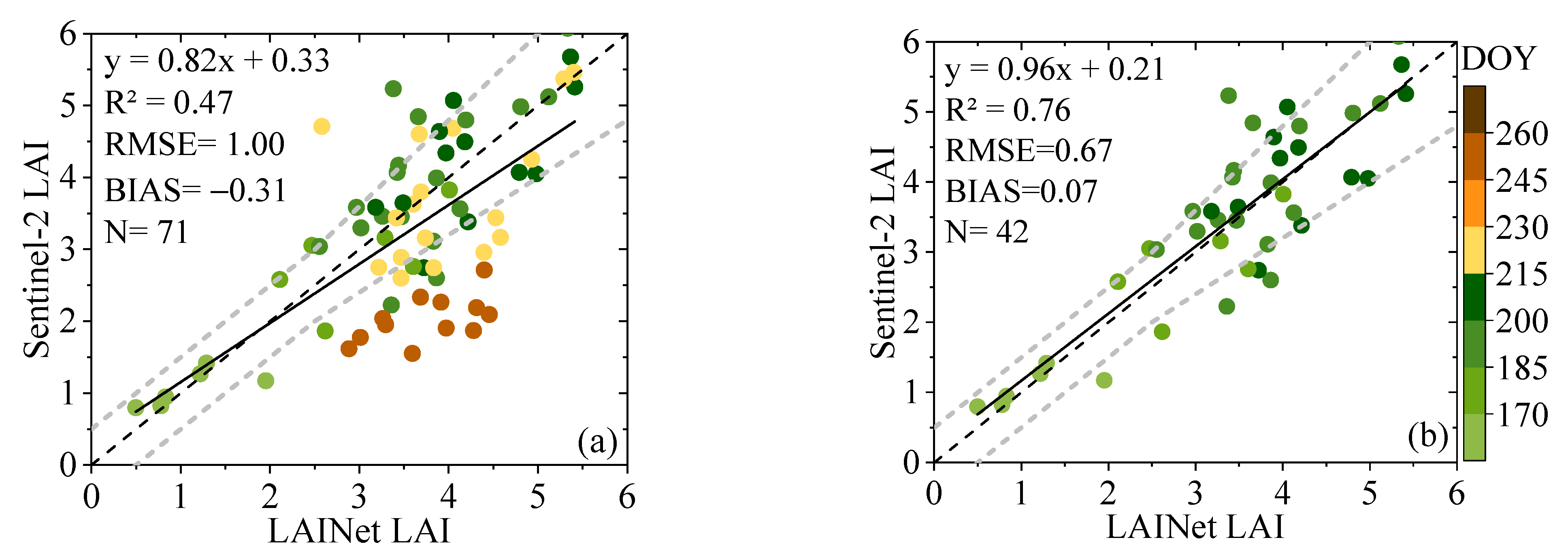
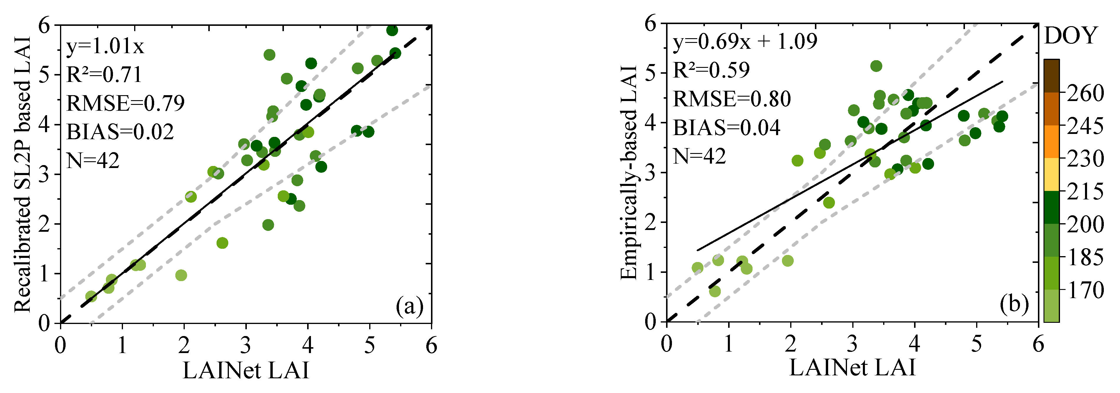
3.1.1. Validation and Recalibration of the Sentinel-2 LAI Product

The Sentinel-2 LAI time series were validated over the entire growing season through direct comparison with LAINet LAI measurements having a similar footprint. Then, a linear regression relationship between the Sentinel-2 and LAINet LAI was fitted and used to recalibrate Sentinel-2 LAI to generate recalibrated SL2P-based LAI.

3.1.2. Generation of Empirically Based LAI

For comparison, the hierarchical up-scaling validation approach proposed by CEOS WGCV was also adopted [15]. The empirical transfer function between LAINet LAI and Sentinel-2 reflectances was established based on an iteratively re-weighted least squares algorithm (IRLS) [56,57,58]. IRLS is a way of mitigating the influence of outliers in an otherwise normally distributed data set and used to find the maximum likelihood estimates of a generalized linear model. IRLS provides lower weight to unreliable ESUs that do not fit well; therefore, the resulting transfer function is less sensitive to outliers in the data as compared with ordinary least squares regression [59].

3.1.3. Assessment of the Reference LAI

A 6-fold cross validation was implemented to assess the reliability of the reference LAI derived from recalibrated SL2P-based and empirically based methods. All the data were randomly divided into six data subsets of the same size. In each iteration, five subsets were used as the training sets, and the remaining subset was used as the test set. The cross-validation process was repeated 6 times and all LAINet LAI were used for both calibration and test processes. Finally, all the test samples at each iteration were integrated to obtain final assessment results.

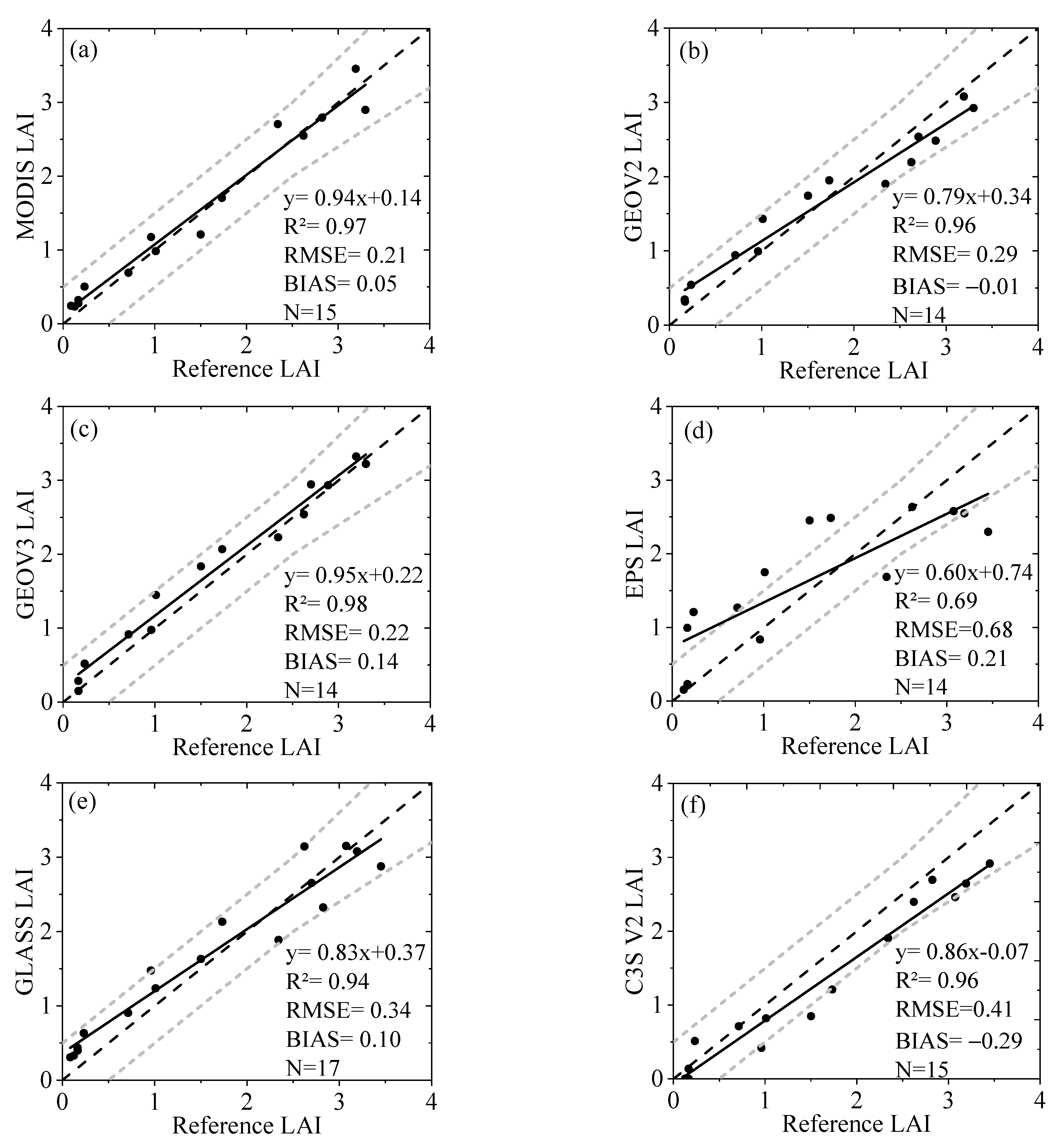
3.2. Validation of the Hectometric and Kilometric LAI Products

The spatial mismatch between the reference decametric LAI and the hectometric and kilometric LAI products is the main issue for the validation [60,61]. In order to mediate geo-mismatch and footprint influence, all the LAI values covered in the 5 km × 5 km study area were averaged, which substantially improved the robustness of the validation at expenses of reducing the number of samples. To reduce the influence of temporal mismatch, only reference-retrieved LAI pairs within 8-day temporal difference were considered.

Three statistical metrics—coefficient of determination (R², Equation (1)), the root mean square error (RMSE, Equation (2)) and the mean difference of the LAI products minus the reference LAI maps (BIAS, Equation (3))—were used to assess the goodness-of-fit, accuracy and systematic deviation, respectively. These metrics are computed as follows:

$$R^2=1-\frac{{\displaystyle {\sum }_{i=1}^N{(y_i-y_i{}^{\prime })}^2}}{{\displaystyle {\sum }_{i=1}^N{(y_i-\overline{y})}^2}}$$

(1)

$$RMSE=\sqrt{\frac{{\displaystyle {\sum }_{i=1}^N{(y_i-y_i{}^{\prime })}^2}}{N}}$$

(2)

$$BIAS=\frac{1}{N}{\displaystyle {\sum }_{i=1}^N(y_i{}^{\prime }-y_i)}$$

(3)

where N is the number of observations, $y_i$ is the reference LAI for the ith observation, $y_i{}^{\prime }$ is the LAI to be validated, $\overline{y}$ is the mean value of reference LAI. The uncertainty threshold established by GCOS, i.e., max (0.5, 20%) [62], was employed as a benchmark to check if the LAI products meet the user requirements.

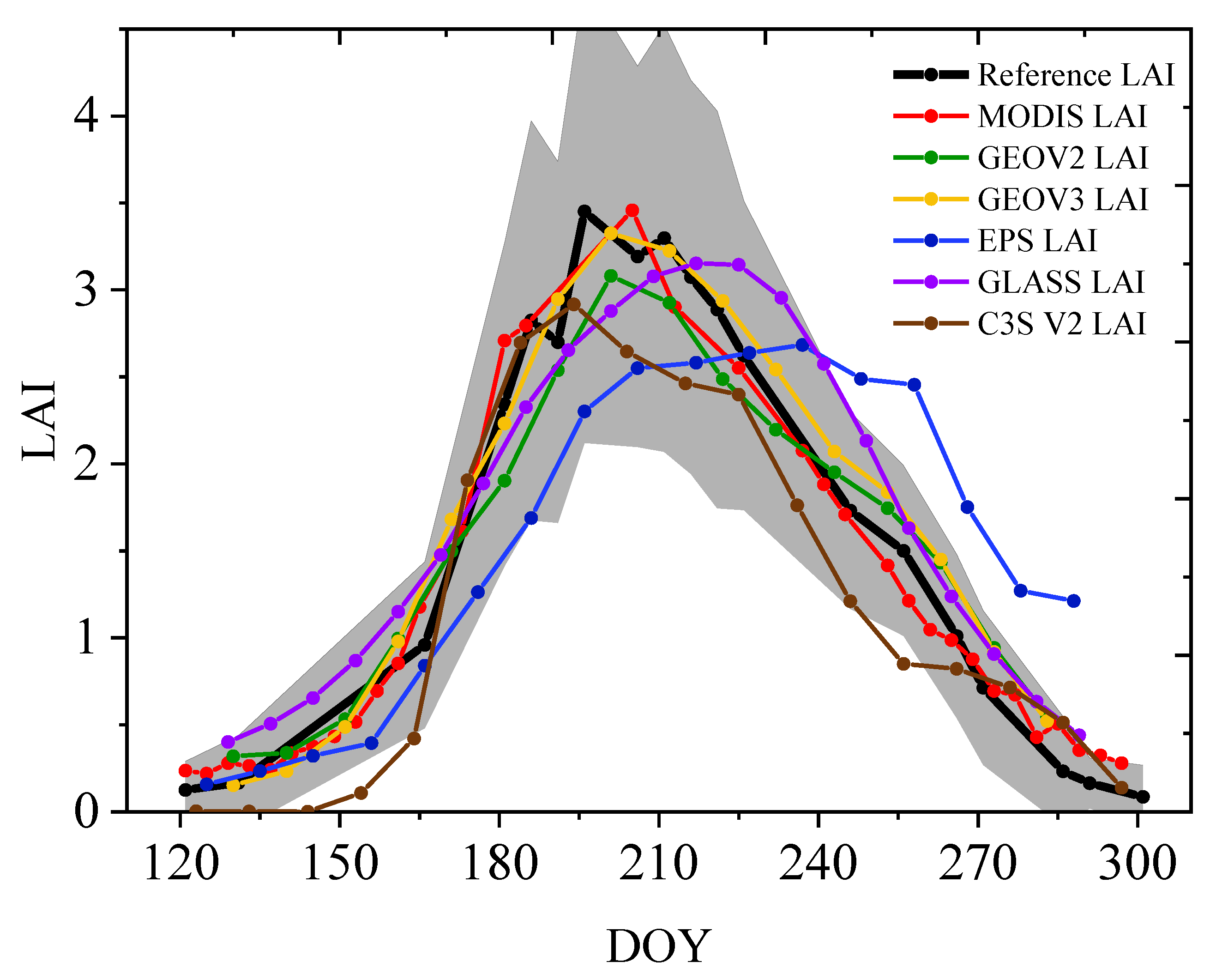
3.3. Validation of the Phenological Metrics

We compared the annual phenological metrics extracted from the hectometric and kilometric LAI products with the phenology from the reference Sentinel-2 LAI time series. Before the extraction of phenological metrics, we applied the Savitzky–Golay (SG) [63] method to smooth time series of reference LAI, hectometric and kilometric LAI products. The SG filter fits local polynomial functions in a temporal moving window. In this paper, a quadratic polynomial SG filter with a time window of 7 days was used. This way, the SG filter captures subtle and rapid changes in the data while being little sensitive to outliers.

The dynamic threshold method was applied to the smoothed time series for the extraction of phenological metrics [64,65]. The start of season (SoS) was defined as the date for which LAI value rises to a given percentage (50% in this study) of its seasonal amplitude. The end of season (EoS) was computed as the date for which LAI value decreases to the same 50% percentage of the amplitude. The peak of season (PoS) was defined as the date for which LAI value rises to the maximum value. The SG filter and the dynamic threshold method are executed in TIMESAT [66] software to extract the SoS, PoS and EoS metrics.

The validation of phenological metrics consists in the comparison of the timing of the SoS, PoS and EoS for the year 2019 as extracted from hectometric and kilometric LAI products vs. the phenological metrics derived from the reference Sentinel-2 LAI time series after smoothing.

4. Results

4.1. Field Measurements

The time series of LAINet at each ESU showed similar temporal patterns (Figure 3). The study area is characterized by a single-growing season. The LAI grows rapidly in the growing period from approximately 0.5 on DOY 152 to 4–5 at the peak of the growing period occurring on DOY 211. After DOY 211, the maize shrinks and matures, and LAI decreases gradually. Some spurious fluctuations are observed mainly close to the peak of the growing season.

4.2. Validation of the Sentinel-2 LAI Product

The Sentinel-2 LAI showed high synchronization with the LAINet LAI during the first half of the growing season (Figure 3). However, Sentinel-2 and LAINet LAI decouple from each other around DOY 211: Sentinel-2 decreases gradually while LAINet LAI values remain high. This decoupling may result from the different definitions of LAI: Only the green elements of plant, i.e., green area index (GAI) are considered when calculating Sentinel-2 LAI [39]. On the other hand, LAINet computes the total plant area index (PAI) [38], i.e., the area index of all vegetated elements including both photosynthetic active and inactive elements. To confirm this hypothesis, the leaf chlorophyll content (CC) of the 5 km × 5 km study area as retrieved from Sentinel-2 by SL2P was assessed (Figure 4). It clearly revealed that CC gradually increased before DOY 211 and monotonically decreased after DOY 211. It implies that leaves began to turn yellow after DOY 211 and this explains why Sentinel-2 LAI and LAINet LAI decouple after then.

Because of the definition discrepancy between the Sentinel-2 LAI product and LAINet LAI, they revealed medium consistency over the entire implementation period of LAINet (R² = 0.47, RMSE = 1.00 and BIAS = −0.31, Figure 5a). To give a physically sound comparison, we eliminated the LAI-pairs after DOY 211 as shown in Figure 5b. As expected, the consistence between the SL2P-based Sentinel-2 LAI and LAINet LAI was substantially improved: R² = 0.76, RMSE = 0.67 and BIAS = 0.07, with most (>80%) of the points in the scatter lie in the GCOS uncertainty requirement (max (0.5, 20%). Our results are in accordance with the studies by [22], which also demonstrated the high accuracy of SL2P-based Sentinel-2 LAI product over crops. Since the definition of hectometric and kilometric LAI products involved in this study also corresponds to GAI, we used only the LAINet values before DOY 211 for recalibrating the Sentinel-2 LAI. The resulting recalibration regression line (y = 0.96x + 0.21) is shown in Figure 5b.

Figure 6 shows the cross-validation results of two types of reference LAI maps. The empirically based LAI yielded an accuracy of R² = 0.59, RMSE = 0.80 and BIAS = 0.04 for all sites. Approximately 55% of the points in the scatter lie in the GCOS uncertainty requirement (max (0.5, 20%)). The recalibrated SL2P-based LAI showed a better performance than the empirically based one, with R² of 0.71, RMSE of 0.79 and BIAS of 0.02; most (>70%) of the points in the scatter lie in the GCOS uncertainty requirement (max (0.5, 20%)).

4.3. Validation of the Hectometric and Kilometric LAI Products

Figure 7 shows the comparisons between the hectometric/kilometric LAI products and the reference LAI. There are differences in the performance of different LAI products due to different input reflectances and retrieval algorithms, but they all show an overall high consistency with the reference LAI (R² > 0.9) except EPS LAI. All the retrieved LAI meet the GCOS uncertainty requirements (i.e., max (0.5, 20%)) except EPS and C3S V2 in few samples (Figure 7). MODIS, GEOV3 and GEOV2 LAI products perform the best among the validated LAI products in our study, with RMSE of 0.21, 0.22 and 0.29, respectively, small bias (BIAS of 0.05, 0.14 and −0.01, respectively) and a high coefficient of determination (R² of 0.97, 0.98 and 0.96, respectively). The GLASS product also performs well in our study area (R² = 0.94, RMSE = 0.34 and BIAS = 0.10). EPS shows the weakest consistency with reference LAI in our study area (R² = 0.69, RMSE = 0.68) and a saturation when LAI is higher than 2.5 (Figure 7d). The C3S product shows high coefficient of determination with the reference LAI (R² = 0.96), whereas it systematically underestimates the reference LAI values (BIAS = −0.29, Figure 7f).

Figure 8 shows the time series of MODIS, GEOV2, GEOV3, EPS, GLASS, C3S V2 and reference LAI during 2019. The gray area in Figure 8 represents the standard deviation calculated from reference LAI. The Copernicus Global Service products GEOV2 and GEOV3 show a high temporal consistency between them (and with reference LAI). MODIS also agrees with reference LAI in terms of seasonality, but it shows some gaps close to the maximum LAI. GLASS LAI is over-smoothed and shows a temporal shift with a delay in the timing of the peak of the growing season. EPS LAI also shows a temporal delay in its seasonality and a high discrepancy compared to reference LAI: the latter half part of EPS time series after the peak of the growing season is outside the confidence interval. The C3S V2 shows an advance in its phenology compared to reference LAI and it provides some values which are out of the confidence interval.

4.4. Validation of the Phenological Metrics

Table 2. Timing (day of year, DOY) for the start of season (SoS), the peak of the growing season (PoS) and the end of season (EoS) for the different LAI products. In parenthesis, the bias in days as compared to the reference LAI phenology is indicated.

Name	SoS	PoS	EoS
Reference LAI	174	207	252
MODIS LAI	172 (−2)	206 (−1)	244 (−8)
GEOV2 LAI	173 (−1)	208 (+1)	256 (+4)
GEOV3 LAI	172 (−2)	208 (+1)	255 (+3)
EPS LAI	180 (+6)	227 (+20)	276 (+24)
GLASS LAI	173 (−1)	216 (+9)	256 (+4)
C3S V2 LAI	170 (−4)	201 (−6)	246 (−6)

lists the SoS, EoS and PoS of different LAI products. The SoS extracted from coarse LAI products is 1–4 days (d) earlier than that of reference LAI except for EPS which is 6 d later. The date for EoS and PoS of coarse resolution LAI products were both later than that of the reference LAI except MODIS and C3S V2 LAI products. C3S V2 shows a systematic advance of −4 d for the SoS and −6 d for the PoS and EoS. EPS LAI product showed the highest differences as compared to the reference LAI with a delay in the timing of phenology metrics: +6d for the SoS, +20 d for the PoS and +24 d for the EoS.

5. Discussion

This validation exercise of decametric, hectometric and kilometric LAI products focus on the assessment of time series over maize crops. The selected area of 5 × 5 km is flat and relatively homogenous, but the maize varieties planted in the different ESUs are different. The types of maize under study should be the same in future experiments to facilitate up-scaling. The spatial homogeneity is an important factor to be considered for the validation of multi-resolution LAI products because the estimation of LAI is scale dependent due to the strong nonlinearity of LAI with reflectance [34,67].

The small fluctuations in the field-measured time series close to the green peak (Figure 3) were also reported in the earlier paper by [68]. There are two potential factors explaining the fluctuations: (1) The changing weather conditions—LAINet uses multiple observations of direct solar light to construct hemispheric gap fraction, and then calculate LAI based on Beer Lambert law [35]. Therefore, the daily variation of the proportion of scattered sky light will cause fluctuation in the time series, specially under partial cloud cover conditions. (2) The crop management activities, e.g., weeding, irrigation and fertilization, may result in a prompt LAI change.

We only used LAINet data for the first half of the growing season given the different definitions of LAI considered to calculate Sentinel-2 LAI (only green elements of the canopy) and LAINet LAI (all elements of the canopy, both photosynthetic active and inactive). The Sentinel-2 LAI before the peak of the growing season (DOY 211) is highly consistent with LAINet LAI (Figure 5b) and clearly improved the performances reported in the previous study [22]. Extending the validation to the entire growing season including senescent period of maize would require having access to ground data from downward looking instruments to account only green elements.

Cross-validation reveals that the proposed up-scaling approach based on the recalibration of existing decametric S2LR Sentinel-2 LAI product with LAINet measurements improved the standard CEOS empirical up-scaling approach. It may constitute an alternative when low ground measurements are available. This methodology may be also applied to other land cover types, but it is limited to the validity of the PROSAIL model used in SL2P algorithm which assumes a turbid medium. In other conditions and over forest areas, in particular, a specific training with a more adapted radiative transfer model would be required.

The MODIS, GEOV2 and GEOV3 LAI products perform the best among all the validated hectometric and kilometric products in our study in terms of RMSE (RMSE = 0.21, 0.22 and 0.29, respectively) and correlation with reference LAI (R² = 0.97, 0.98 and 0.96, respectively). The MODIS LAI time series show some gaps close to the maximum peak of the growing season mainly due to cloud and other poor atmospheric conditions [69,70], which were filtered out through the quality control procedure [47]. The MODIS LAI is generated based on a simple compositing approach of the daily LAI estimates in an 8-day window whilst the other analyzed products use more elaborated compositing techniques either at the level of LAI estimates (GEOV2 and GEOV3) or input reflectances (EPS, GLASS and C3S V2) with longer and adaptive temporal windows as described in Section 2.2. The similarity of GEOV2 and GEOV3 time series can be explained because the two versions of products are retrieved from the same sensor (PROBA-V) and preprocessing chain, and both are based on the use of a similar NNs retrieval approach and smoothing temporal filters and compositing [51]. The GLASS product showed the smoothest temporal evolution but clear artifacts in terms of phenology (Figure 8) with a delay in the second half of the growing season after the peak of LAI as compared to the reference time series. This may be introduced by an over-smoothing in the reprocessed MODIS reflectances which are used as input of the GLASS algorithm (Section 2.2.6). The EPS product showed clear deficiencies to reproduce the seasonality of reference LAI time series with a delay in its phenology (Figure 8) and an underestimation for LAI > 3 (Figure 7). The underestimation of EPS LAI product may indicate an early saturation of the retrieval algorithm [11]. The C3S V2 LAI product also showed systematic differences with reference LAI both for the seasonality: advanced phenology, and LAI magnitude: systematic underestimation of the reference LAI values for the entire range 0–3.5 LAI and especially for low LAI values (<0.5) at the start of growing season and high LAI values (>3.0) at the peak of growing season and after senescent (Figure 8). Pinty et al. [71] attributed the high uncertainty of LAI derived from TIP model for the small and high values to the observational uncertainties and the saturation effects, respectively. Note, however, that the GEOV2 and GEOV3 products derived from the same PROBA-V data, as C3S did not show these artifacts and they improved the C3S V2 product when compared with the reference LAI both in terms of the LAI magnitude and phenology.

The hectometric and kilometric LAI products showed an earlier SoS as compared to the reference LAI from decametric Sentinel-2. This may be explained by the spatial heterogeneity and the presence of species with earlier growing seasons in the study area. The main planting crop in the study area is maize, but since it is planted by individual farmers, it is inevitable to be covered by other crops planted in a small range or weeds. The coarse resolution satellites may result more sensitive than high resolution satellites to the presence of species with an earlier SoS [72]. The comparison between LAI products and with reference LAI time series show important differences in terms of phenology with apparent limitations for EPS, C3SV2 and GLASS which exhibit systematic differences in the timing of phenological metrics as compared to other products and reference LAI. However, phenological ground measurements are not available in our study area. Further validation and comparison with ground-based phenology will be conducted in future studies to directly validate the satellite phenological metrics.

6. Conclusions

We proposed a direct approach to validate coarse resolution LAI products that involved the scaling up of field-measured LAI via the validation and recalibration of the Sentinel-2 LAI product. MODIS, GEOV3 and GEOV2 LAI products showed good performance in the magnitude of LAI (RMSE < 0.3) and the timing of phenology metrics in maize crops (within −2 d difference for the timing of the start of season (SoS), ±1 d for the peak of season (PoS) and ±8 d for the end of season (EoS)). EPS LAI showed, on the opposite, high differences in terms of magnitude of LAI with an underestimation of high LAI values, R² = 0.69 and RMSE = 0.68, and a delay in the timing of phenology metrics as compared to other products and the reference LAI (+6 d for the SoS, +20 d for the PoS and +24 d for the EoS). GLASS also showed a delay in the second half of the growing season after the peak of LAI. C3S V2 showed high correlation with reference LAI values but a systematic underestimation of LAI values with a negative BIAS of −0.29 LAI and a systematic advance of −4d for the SoS and −6d for the PoS and EoS. More validation activities and comparison with ground-based phenological metrics are necessary to further verify these findings. This study demonstrated the potential of using the decametric Sentinel-2 LAI product with minimum ground-based calibration as a reference to validate the hectometric and kilometric LAI products over cropland areas. This approach may constitute an alternative to the standard CEOS up-scaling approach when a limited number of ground measurements are available. The methodology may also be applied to other land cover types, but it is limited to the conditions of validity of the physical model used for training Sentinel-2 LAI.

References

1. Chen, J.M.; Black, T.A. Defining leaf area index for non-flat leaves. Plant Cell Environ. 1992, 15, 421–429. [Google Scholar] [CrossRef]
2. Fang, H.; Baret, F.; Plummer, S.; Schaepman-Strub, G. An Overview of Global Leaf Area Index (LAI): Methods, Products, Validation, and Applications. Rev. Geophys. 2019, 57, 739–799. [Google Scholar] [CrossRef]
3. Fang, H.; Zhang, Y.; Wei, S.; Li, W.; Ye, Y.; Sun, T.; Liu, W. Validation of global moderate resolution leaf area index (LAI) products over croplands in northeastern China. Remote Sens. Environ. 2019, 233, 111377. [Google Scholar] [CrossRef]
4. Verrelst, J.; Malenovský, Z.; van der Tol, C.; Camps-Valls, G.; Gastellu-Etchegorry, J.P.; Lewis, P.; North, P.; Moreno, J. Quantifying Vegetation Biophysical Variables from Imaging Spectroscopy Data: A Review on Retrieval Methods. Surv. Geophys. 2019, 40, 589–629. [Google Scholar] [CrossRef] [Green Version]
5. Le Maire, G.; François, C.; Soudani, K.; Berveiller, D.; Pontailler, J.-Y.; Bréda, N.; Genet, H.; Davi, H.; Dufrêne, E. Calibration and validation of hyperspectral indices for the estimation of broadleaved forest leaf chlorophyll content, leaf mass per area, leaf area index and leaf canopy biomass. Remote Sens. Environ. 2008, 112, 3846–3864. [Google Scholar] [CrossRef]
6. Danner, M.; Berger, K.; Wocher, M.; Mauser, W.; Hank, T. Efficient RTM-based training of machine learning regression algorithms to quantify biophysical & biochemical traits of agricultural crops. ISPRS J. Photogramm. Remote Sens. 2021, 173, 278–296. [Google Scholar] [CrossRef]
7. Verger, A.; Baret, F.; Camacho, F. Optimal modalities for radiative transfer-neural network estimation of canopy biophysical characteristics: Evaluation over an agricultural area with CHRIS/PROBA observations. Remote Sens. Environ. 2011, 115, 415–426. [Google Scholar] [CrossRef]
8. Yan, K.; Park, T.; Yan, G.; Chen, C.; Yang, B.; Liu, Z.; Nemani, R.R.; Knyazikhin, Y.; Myneni, R.B. Evaluation of MODIS LAI/FPAR Product Collection 6. Part 1: Consistency and Improvements. Remote Sens. 2016, 8, 359. [Google Scholar] [CrossRef] [Green Version]
9. Verger, A.; Baret, F.; Weiss, M. Algorithm Theorethical Basis Document. Leaf Area Index (LAI) Fraction of Absorbed Photosynthetically Active Radiation (FAPAR) Fraction of green Vegetation Cover (FCover) Collection 1 km Version 2. 2019. Available online: https://land.copernicus.eu/global/sites/cgls.vito.be/files/products/CGLOPS1_ATBD_LAI1km-V2_I1.41.pdf (accessed on 4 November 2021).
10. Baret, F.; Weiss, M.; Verger, A.; Smets, B. ATBD for LAI, FAPAR and FCOVER from PROBA-V Products at 300M Resolution (GEOV3). 2013. Available online: http://fp7-imagines.eu/pages/documents.php (accessed on 4 November 2021).
11. Haro, F.J.G.; Campos-Taberner, M.; Muñoz-Marí, J.; Laparra, V.; Camacho, F.; Sánchez-Zapero, J.; Camps-Valls, G. Derivation of global vegetation biophysical parameters from EUMETSAT Polar System. ISPRS J. Photogramm. Remote Sens. 2018, 139, 57–74. [Google Scholar] [CrossRef]
12. Xiao, Z.; Liang, S.; Wang, J.; Xiang, Y.; Zhao, X.; Song, J. Long-Time-Series Global Land Surface Satellite Leaf Area Index Product Derived From MODIS and AVHRR Surface Reflectance. IEEE Trans. Geosci. Remote Sens. 2016, 54, 5301–5318. [Google Scholar] [CrossRef]
13. Blessing, S.; Giering, R. Algorithm Theoretical Basis Document PROBA-V CDR and ICDR LAI and fAPAR v2.0. 2019. Available online: https://datastore.copernicus-climate.eu/documents/satellite-lai-fapar/D1.4.3-v2.0_ATBD_CDR-ICDR_LAI_FAPAR_PROBAV_v2.0_PRODUCTS_v1.0.pdf (accessed on 4 November 2021).
14. Morisette, J.; Baret, F.; Privette, J.; Myneni, R.; Nickeson, J.; Garrigues, S.; Shabanov, N.; Weiss, M.; Fernandes, R.; Leblanc, S.; et al. Validation of global moderate-resolution LAI products: A framework proposed within the CEOS land product validation subgroup. IEEE Trans. Geosci. Remote Sens. 2006, 44, 1804–1817. [Google Scholar] [CrossRef] [Green Version]
15. Fernandes, R.; Plummer, S.; Nightingale, J.; Baret, F.; Camacho, F.; Fang, H.; Garrigues, S.; Gobron, N. Global Leaf Area Index Product Validation Good Practices. Version 2.0; 2014. Available online: https://lpvs.gsfc.nasa.gov/PDF/CEOS_LAI_PROTOCOL_Aug2014_v2.0.1.pdf (accessed on 4 November 2021).
16. Yin, G.; Li, A.; Zeng, Y.; Xu, B.; Zhao, W.; Nan, X.; Jin, H.; Bian, J. A Cost-Constrained Sampling Strategy in Support of LAI Product Validation in Mountainous Areas. Remote Sens. 2016, 8, 704. [Google Scholar] [CrossRef] [Green Version]
17. Mayr, M.J.; Samimi, C. Comparing the Dry Season In-Situ Leaf Area Index (LAI) Derived from High-Resolution RapidEye Imagery with MODIS LAI in a Namibian Savanna. Remote Sens. 2015, 7, 4834–4857. [Google Scholar] [CrossRef] [Green Version]
18. Jin, H.; Li, A.; Bian, J.; Nan, X.; Zhao, W.; Zhang, Z.; Yin, G. Intercomparison and validation of MODIS and GLASS leaf area index (LAI) products over mountain areas: A case study in southwestern China. Int. J. Appl. Earth Obs. Geoinf. 2017, 55, 52–67. [Google Scholar] [CrossRef]
19. Brown, L.A.; Meier, C.; Morris, H.; Pastor-Guzman, J.; Bai, G.; Lerebourg, C.; Gobron, N.; Lanconelli, C.; Clerici, M.; Dash, J. Evaluation of global leaf area index and fraction of absorbed photosynthetically active radiation products over North America using Copernicus Ground Based Observations for Validation data. Remote Sens. Environ. 2020, 247, 111935. [Google Scholar] [CrossRef]
20. De Kauwe, M.; Disney, M.; Quaife, T.; Lewis, P.; Williams, M. An assessment of the MODIS collection 5 leaf area index product for a region of mixed coniferous forest. Remote Sens. Environ. 2011, 115, 767–780. [Google Scholar] [CrossRef]
21. Fang, H.; Wei, S.; Liang, S. Validation of MODIS and CYCLOPES LAI products using global field measurement data. Remote Sens. Environ. 2012, 119, 43–54. [Google Scholar] [CrossRef]
22. Djamai, N.; Fernandes, R.; Weiss, M.; McNairn, H.; Goïta, K. Validation of the Sentinel Simplified Level 2 Product Prototype Processor (SL2P) for mapping cropland biophysical variables using Sentinel-2/MSI and Landsat-8/OLI data. Remote Sens. Environ. 2019, 225, 416–430. [Google Scholar] [CrossRef]
23. Hu, Q.; Yang, J.; Xu, B.; Huang, J.; Memon, M.S.; Yin, G.; Zeng, Y.; Zhao, J.; Liu, K. Evaluation of Global Decametric-Resolution LAI, FAPAR and FVC Estimates Derived from Sentinel-2 Imagery. Remote Sens. 2020, 12, 912. [Google Scholar] [CrossRef] [Green Version]
24. Jin, H.; Li, A.; Yin, G.; Xiao, Z.; Bian, J.; Nan, X.; Jing, J. A Multiscale Assimilation Approach to Improve Fine-Resolution Leaf Area Index Dynamics. IEEE Trans. Geosci. Remote Sens. 2019, 57, 8153–8168. [Google Scholar] [CrossRef]
25. Fang, H.; Liang, S.; Townshend, J.; Dickinson, R. Spatially and temporally continuous LAI data sets based on an integrated filtering method: Examples from North America. Remote Sens. Environ. 2008, 112, 75–93. [Google Scholar] [CrossRef]
26. Garrigues, S.; Shabanov, N.; Swanson, K.; Morisette, J.; Baret, F.; Myneni, R. Intercomparison and sensitivity analysis of Leaf Area Index retrievals from LAI-2000, AccuPAR, and digital hemispherical photography over croplands. Agric. For. Meteorol. 2008, 148, 1193–1209. [Google Scholar] [CrossRef] [Green Version]
27. Demarez, V.; Duthoit, S.; Baret, F.; Weiss, M.; Dedieu, G. Estimation of leaf area and clumping indexes of crops with hemispherical photographs. Agric. For. Meteorol. 2008, 148, 644–655. [Google Scholar] [CrossRef] [Green Version]
28. Leblanc, S.G. Correction to the plant canopy gap-size analysis theory used by the Tracing Radiation and Architecture of Canopies instrument. Appl. Opt. 2002, 41, 7667–7670. [Google Scholar] [CrossRef] [PubMed]
29. LI-COR. LAI-2000 Plant Canopy Analyzer Operating Manual. 1991. Available online: https://licor.app.boxenterprise.net/s/q6hrj6s79psn7o8z2b2s (accessed on 4 November 2021).
30. Jonckheere, I.; Fleck, S.; Nackaerts, K.; Muys, B.; Coppin, P.; Weiss, M.; Baret, F. Review of methods for in situ leaf area index determination: Part I. Theories, sensors and hemispherical photography. Agric. For. Meteorol. 2004, 121, 19–35. [Google Scholar] [CrossRef]
31. Hart, J.K.; Martinez, K. Environmental Sensor Networks: A revolution in the earth system science? Earth-Science Rev. 2006, 78, 177–191. [Google Scholar] [CrossRef] [Green Version]
32. Xiao, Z.; Liang, S.; Wang, J.; Chen, P.; Yin, X.; Zhang, L.; Song, J. Use of General Regression Neural Networks for Generating the GLASS Leaf Area Index Product From Time-Series MODIS Surface Reflectance. IEEE Trans. Geosci. Remote Sens. 2014, 52, 209–223. [Google Scholar] [CrossRef]
33. Yin, G.; Li, A.; Jin, H.; Zhao, W.; Bian, J.; Qu, Y.; Zeng, Y.; Xu, B. Derivation of temporally continuous LAI reference maps through combining the LAINet observation system with CACAO. Agric. For. Meteorol. 2017, 233, 209–221. [Google Scholar] [CrossRef]
34. Yin, G.; Li, J.; Liu, Q.; Li, L.; Zeng, Y.; Xu, B.; Yang, L.; Zhao, J. Improving Leaf Area Index Retrieval Over Heterogeneous Surface by Integrating Textural and Contextual Information: A Case Study in the Heihe River Basin. IEEE Geosci. Remote Sens. Lett. 2014, 12, 359–363. [Google Scholar] [CrossRef]
35. Qu, Y.; Zhu, Y.; Han, W.; Wang, J.; Ma, M. Crop Leaf Area Index Observations With a Wireless Sensor Network and Its Potential for Validating Remote Sensing Products. IEEE J. Sel. Top. Appl. Earth Obs. Remote Sens. 2013, 7, 431–444. [Google Scholar] [CrossRef]
36. Kaminski, T.; Pinty, B.; Voßbeck, M.; Lopatka, M.; Gobron, N.; Robustelli, M. Consistent EO Land Surface Products including Uncertainty Estimates. Biogeosciences Discuss. 2016, 1–28. [Google Scholar] [CrossRef]
37. Qu, Y.; Sun, G. Research on wireless sensor node for measurement of vegetation structure parameters. In Proceedings of the 2010 World Automation Congress, WAC 2010, Kobe, Japan, 19–23 September 2010. [Google Scholar]
38. Qu, Y.; Han, W.; Fu, L.; Li, C.; Song, J.; Zhou, H.; Bo, Y.; Wang, J. LAINet–A wireless sensor network for coniferous forest leaf area index measurement: Design, algorithm and validation. Comput. Electron. Agric. 2014, 108, 200–208. [Google Scholar] [CrossRef]
39. Weiss, M.; Baret, F. S2ToolBox Level 2 Products: LAI, FAPAR, FCOVER. Version 1.1. 2016. Available online: http://step.esa.int/docs/extra/ATBD_S2ToolBox_L2B_V1.1.pdf (accessed on 4 November 2021).
40. Myneni, R.B. MODIS Collection 6 (C6) LAI/FPAR Product User’s Guide. 2020. Available online: https://lpdaac.usgs.gov/documents/624/MOD15_User_Guide_V6.pdf (accessed on 4 November 2021).
41. Verger, A.; Baret, F.; Weiss, M. Near Real-Time Vegetation Monitoring at Global Scale. IEEE J. Sel. Top. Appl. Earth Obs. Remote Sens. 2014, 7, 3473–3481. [Google Scholar] [CrossRef]
42. Verger, A.; Filella, I.; Baret, F.; Penuelas, J. Vegetation baseline phenology from kilometric global LAI satellite products. Remote Sens. Environ. 2016, 178, 1–14. [Google Scholar] [CrossRef] [Green Version]
43. MuellerWilm, U.; Devignot, O.; Pessiot, L. Sen2Cor Configuration and User Manual. Sen2Cor Software Release Note. 2019. Available online: http://step.esa.int/thirdparties/sen2cor/2.5.5/docs/S2-PDGS-MPC-L2A-SUM-V2.5.5_V2.pdf (accessed on 4 November 2021).
44. Jacquemoud, S.; Verhoef, W.; Baret, F.; Bacour, C.; Zarco-Tejada, P.J.; Asner, G.P.; François, C.; Ustin, S.L. PROSPECT+SAIL models: A review of use for vegetation characterization. Remote Sens. Environ. 2009, 113, S56–S66. [Google Scholar] [CrossRef]
45. Myneni, R.B.; Hoffman, S.; Knyazikhin, Y.; Privette, J.L.; Glassy, J.; Tian, Y.; Wang, Y.; Song, X.; Zhang, Y.; Smith, G.R.; et al. Global products of vegetation leaf area and fraction absorbed PAR from year one of MODIS data. Remote Sens. Environ. 2002, 83, 214–231. [Google Scholar] [CrossRef] [Green Version]
46. Wang, Y.; Tian, Y.; Zhang, Y.; El-Saleous, N.; Knyazikhin, Y.; Vermote, E.; Myneni, R.B. Investigation of product accuracy as a function of input and model uncertainties: Case study with SeaWiFS and MODIS LAI/FPAR algorithm. Remote Sens. Environ. 2001, 78, 299–313. [Google Scholar] [CrossRef]
47. Yan, K.; Park, T.; Yan, G.; Liu, Z.; Yang, B.; Chen, C.; Nemani, R.R.; Knyazikhin, Y.; Myneni, R.B. Evaluation of MODIS LAI/FPAR Product Collection 6. Part 2: Validation and Intercomparison. Remote Sens. 2016, 8, 460. [Google Scholar] [CrossRef] [Green Version]
48. Baret, F.; Hagolle, O.; Geiger, B.; Bicheron, P.; Miras, B.; Huc, M.; Berthelot, B.; Niño, F.; Weiss, M.; Samain, O.; et al. LAI, fAPAR and fCover CYCLOPES global products derived from VEGETATION: Part 1: Principles of the algorithm. Remote Sens. Environ. 2007, 110, 275–286. [Google Scholar] [CrossRef] [Green Version]
49. Verger, A.; Baret, F.; Weiss, M.; Kandasamy, S.; Vermote, E. The CACAO Method for Smoothing, Gap Filling, and Characterizing Seasonal Anomalies in Satellite Time Series. IEEE Trans. Geosci. Remote Sens. 2013, 51, 1963–1972. [Google Scholar] [CrossRef]
50. Smets, B.; Jacobs, T.; Verger, A. Leaf Area Index (LAI) Fraction of Photosynthetically Active Radiation (FAPAR) Fraction of Vegetation Cover (FCOVER) Collection 300M Version 1. 2018. Available online: https://land.copernicus.eu/global/sites/cgls.vito.be/files/products/GIOGL1_PUM_LAI300m-V1_I1.60.pdf (accessed on 4 November 2021).
51. Fuster, B.; Sánchez-Zapero, J.; Camacho, F.; García-Santos, V.; Verger, A.; Lacaze, R.; Weiss, M.; Baret, F.; Smets, B. Quality Assessment of PROBA-V LAI, fAPAR and fCOVER Collection 300 m Products of Copernicus Global Land Service. Remote Sens. 2020, 12, 1017. [Google Scholar] [CrossRef] [Green Version]
52. Chen, J.M. Optically-based methods for measuring seasonal variation of leaf area index in boreal conifer stands. Agric. For. Meteorol. 1996, 80, 135–163. [Google Scholar] [CrossRef]
53. Tang, H.; Yu, K.; Hagolle, O.; Jiang, K.; Geng, X.; Zhao, Y. A cloud detection method based on a time series of MODIS surface reflectance images. Int. J. Digit. Earth 2013, 6, 157–171. [Google Scholar] [CrossRef]
54. Baret, F.; Morissette, J.; Fernandes, R.; Champeaux, J.; Myneni, R.; Chen, J.; Plummer, S.; Weiss, M.; Bacour, C.; Garrigues, S.; et al. Evaluation of the representativeness of networks of sites for the global validation and intercomparison of land biophysical products: Proposition of the CEOS-BELMANIP. IEEE Trans. Geosci. Remote Sens. 2006, 44, 1794–1803. [Google Scholar] [CrossRef]
55. Pinty, B.; Lavergne, T.; Dickinson, R.E.; Widlowski, J.-L.; Gobron, N.; Verstraete, M.M. Simplifying the interaction of land surfaces with radiation for relating remote sensing products to climate models. J. Geophys. Res. Space Phys. 2006, 111, 111. [Google Scholar] [CrossRef] [Green Version]
56. Street, J.O.; Carroll, R.J.; Ruppert, D. A Note on Computing Robust Regression Estimates via Iteratively Reweighted Least Squares. Am. Stat. 1988, 42, 152–154. [Google Scholar] [CrossRef] [Green Version]
57. DuMouchel, W.; O’Brien, F. Integrating a Robust Option into a Multiple Regression Computing Environment. IMA Vol. Math. Its Appl. 1992, 41–48. [Google Scholar] [CrossRef]
58. Holland, P.W.; Welsch, R.E. Robust regression using iteratively reweighted least-squares. Commun. Stat.-Theory Methods 1977, 6, 813–827. [Google Scholar] [CrossRef]
59. Rossello, P. Ground Data Processing & Production of the Level 1 High Resolution Maps. 2007. Available online: http://w3.avignon.inra.fr/valeri/amerique-du-sud/guyane/2001/biomap/Counami2001FTReport.pdf (accessed on 4 November 2021).
60. Weiss, M.; Baret, F.; Garrigues, S.; Lacaze, R. LAI and fAPAR CYCLOPES Global Products Derived from VEGETATION. Part 2: Validation and Comparison with MODIS Collection 4 Products. Remote Sens. Environ. 2007, 110, 317–331. [Google Scholar] [CrossRef]
61. Baret, F.; Weiss, M.; Lacaze, R.; Camacho, F.; Makhmara, H.; Pacholcyzk, P.; Smets, B. GEOV1: LAI and FAPAR essential climate variables and FCOVER global time series capitalizing over existing products. Part1: Principles of development and production. Remote Sens. Environ. 2013, 137, 299–309. [Google Scholar] [CrossRef]
62. GCOS. Systematic Observation Requirements for Satellite-Based Products for Climate, 2011 Update, Supplemental Details to the Satellite-Based Component of the Implementation Plan for the Global Observing System for Climate in Support of the UNFCCC (2010 Update). 2011. Available online: https://library.wmo.int/index.php?lvl=notice_display&id=12907 (accessed on 4 November 2021).
63. Savitzky, A.; Golay, M.J.E. Smoothing and Differentiation of Data by Simplified Least Squares Procedures. Anal. Chem. 1964, 36, 1627–1639. [Google Scholar] [CrossRef]
64. Yu, H.; Luedeling, E.; Xu, J. Winter and spring warming result in delayed spring phenology on the Tibetan Plateau. Proc. Natl. Acad. Sci. USA 2010, 107, 22151–22156. [Google Scholar] [CrossRef] [Green Version]
65. White, M.; Thornton, P.; Running, S.W. A continental phenology model for monitoring vegetation responses to interannual climatic variability. Glob. Biogeochem. Cycles 1997, 11, 217–234. [Google Scholar] [CrossRef]
66. Jönsson, P.; Eklundh, L. TIMESAT—A program for analyzing time-series of satellite sensor data. Comput. Geosci. 2004, 30, 833–845. [Google Scholar] [CrossRef] [Green Version]
67. Huang, J.; Sedano, F.; Huang, Y.; Ma, H.; Li, X.; Liang, S.; Tian, L.; Zhang, X.; Fan, J.; Wu, W. Assimilating a synthetic Kalman filter leaf area index series into the WOFOST model to improve regional winter wheat yield estimation. Agric. For. Meteorol. 2016, 216, 188–202. [Google Scholar] [CrossRef]
68. Yu, L.; Shang, J.; Cheng, Z.; Gao, Z.; Wang, Z.; Tian, L.; Wang, D.; Che, T.; Jin, R.; Liu, J.; et al. Assessment of Cornfield LAI Retrieved from Multi-Source Satellite Data Using Continuous Field LAI Measurements Based on a Wireless Sensor Network. Remote Sens. 2020, 12, 3304. [Google Scholar] [CrossRef]
69. Garrigues, S.; Lacaze, R.; Baret, F.; Morisette, J.T.; Weiss, M.; Nickeson, J.E.; Fernandes, R.; Plummer, S.; Shabanov, N.V.; Myneni, R.; et al. Validation and intercomparison of global Leaf Area Index products derived from remote sensing data. J. Geophys. Res. Space Phys. 2008, 113. [Google Scholar] [CrossRef]
70. Camacho, F.; Cernicharo, J.; Lacaze, R.; Baret, F.; Weiss, M. GEOV1: LAI, FAPAR essential climate variables and FCOVER global time series capitalizing over existing products. Part 2: Validation and intercomparison with reference products. Remote Sens. Environ. 2013, 137, 310–329. [Google Scholar] [CrossRef]
71. Pinty, B.; Andredakis, I.; Clerici, M.; Kaminski, T.; Taberner, M.; Verstraete, M.; Gobron, N.; Plummer, S.; Widlowski, J.-L. Exploiting the MODIS albedos with the Two-stream Inversion Package (JRC-TIP): 1. Effective leaf area index, vegetation, and soil properties. J. Geophys. Res. Space Phys. 2011, 116. [Google Scholar] [CrossRef]
72. Zhang, X.; Wang, J.; Gao, F.; Liu, Y.; Schaaf, C.; Friedl, M.; Yu, Y.; Jayavelu, S.; Gray, J.; Liu, L. Exploration of scaling effects on coarse resolution land surface phenology. Remote Sens. Environ. 2017, 190, 318–330. [Google Scholar] [CrossRef] [Green Version]
Figure 1. Sentinel-2 false-color RGB (8, 4, 3) composite of the study area on 30 July 2019. The yellow dots indicate the locations of the Elementary Sampling Units (ESUs).
Remotesensing 13 04529 g001
Figure 2. Flowchart of the multi-resolution LAI products validation. First, the SL2P-based Sentinel-2 LAI product was validated and recalibrated with ground measurements from LAINet. The recalibrated SL2P LAI was compared with an empirically based LAI resulting from up-scaling LAINet measurements with Sentinel-2 reflectance data thought the iteratively re-weighted least squares algorithm (IRLS). This resulted in reference maps. Second, hectometric and kilometric LAI products were validated by comparison with the reference maps. Third, phenological metrics from hectometric/kilometric and reference LAI time series were extracted and compared.
Remotesensing 13 04529 g002
Figure 3. Time series of original Sentinel-2 LAI product (points) and LAINet (solid line) measurements for the six elementary sampling units (af) as indicated in Figure 1. The vertical dashed line at day of year (DOY) 211 indicates the timing of the maximum leaf development in our study area.
Remotesensing 13 04529 g003
Figure 4. Time series of leaf chlorophyll content (CC) retrieved from Sentinel-2 by the Simplified Level 2 Product Prototype Processor (SL2P). The dashed line indicates day of year (DOY) 211, when CC began to decrease, i.e., leaf began to turn yellow in our study area.
Remotesensing 13 04529 g004
Figure 5. Comparison between the Sentinel-2 LAI and LAINet for (a) the entire time period (from day of year (DOY) 152 to 263) and (b) for the green-up period (from DOY 152 to 211). The black dashed line indicates 1:1 line, and solid line indicates linear regressions between Sentinel-2 LAI and LAINet. The gray dashed lines show the Global Climate Observing System uncertainty requirements for LAI (max (0.5, 20%)).
Remotesensing 13 04529 g005
Figure 6. Cross-validation between LAINet LAI and (a) the recalibrated SL2P-based LAI, (b) the empirically based LAI for the green-up season (from day of year (DOY) 152 to 211). The black dashed line indicates the 1:1 line, the solid line indicates the linear regression, and the gray dashed lines show the Global Climate Observing System uncertainty requirements for LAI (max (0.5, 20%)).
Remotesensing 13 04529 g006
Figure 7. Comparison between (a) MODIS, (b) GEOV2, (c) GEOV3, (d) EPS, (e) GLASS and (f) C3S V2 with the reference LAI. The black dashed line indicates 1:1 line, and solid line indicates linear regressions between LAI products and reference LAI. The gray dashed lines show the Global Climate Observing System uncertainty requirements for LAI (max (0.5, 20%)).
Remotesensing 13 04529 g007
Figure 8. Time series of reference LAI, MODIS, GEOV2, GEOV3, EPS, GLASS and C3S V2 LAI products. The shaded gray area represents the uncertainty of reference LAI.
Remotesensing 13 04529 g008