Abstract
Accurate and seamless vehicle positioning is fundamental for autonomous driving tasks in urban environments, requiring the provision of high-end measuring devices. Light Detection and Ranging (lidar) sensors, together with Global Navigation Satellite Systems (GNSS) receivers, are therefore commonly found onboard modern vehicles. In this paper, we propose an integration of lidar and GNSS code measurements at the observation level via a mixed measurement model. An Extended Kalman-Filter (EKF) is implemented to capture the dynamic of the vehicle movement, and thus, to incorporate the vehicle velocity parameters into the measurement model. The lidar positioning component is realized using point cloud registration through a deep neural network, which is aided by a high definition (HD) map comprising accurately georeferenced scans of the road environments. Experiments conducted in a densely built-up environment show that, by exploiting the abundant measurements of GNSS and high accuracy of lidar, the proposed vehicle positioning approach can maintain centimeter-to meter-level accuracy for the entirety of the driving duration in urban canyons.
1. Introduction
Accurate and seamless positioning in urban environments is fundamental for autonomous vehicle and driving systems, where minimum human intervention is required to perform driving tasks [1,2]. The term ‘accurate’ indicates that the positioning solution should agree with the vehicle’s true position up to a meter to a few centimeter-levels, while the term ‘seamless’ indicates that delivering such an accurate solution should be maintained during the period of positioning. The provision of positioning solutions, with such stringent requirements, demands the utilization of multiple measuring devices. This is because each device possesses its own distinctive characteristics, thus imposing limitations which need to be overcome through the integration of the device with other devices offering ‘complementary’ characteristics. For instance, while Global Navigation Satellite System (GNSS) receivers are capable of positioning the vehicle with respect to a global reference coordinate frame, they are vulnerable to signal blockages, the Earth’s atmosphere, and errors caused by multipath effects in urban canyons [3,4]. On the other hand, Light Detection and Ranging (lidar) sensors are not subject to signal blockages and multipath, but conventional lidar approaches based on odometry or Simultaneous Localization and Mapping (SLAM) offer positioning solutions relative to a local coordinate frame [5]. The present study aims to explore the performance of lidar, in standalone and in combination with GNSS, for vehicle positioning in deep urban environments. Although we confine our study here to lidar-GNSS integration, it should be remarked that an autonomous vehicle is also equipped with further positioning devices such as Inertial Measurement Unit (IMU) and vision-based (camera) sensors. They allow one to time-predict the vehicle’s position through its previously determined solution and the dynamic of the vehicle’s movement. Such methods do, however, suffer from accumulated errors or drifts over time [6].
As a crucial positioning method, GNSS has recently benefited from the large number of satellites provided by multiple constellations such as the Global Positioning System (GPS), GLONASS, Beidou and Galileo [7,8]. When augmented by a ground-based positioning infrastructure (e.g., a network of reference stations), a single GNSS receiver can deliver carrier-phase-based relative positioning solutions at the centimeter-level [9]. Using a network of eight reference stations, Humphreys et al. [10] have in fact demonstrated the success of such high-precision positioning performance in deep urban areas. However, carrier-phase-based relative positioning requires the provision of a dense reference network which cannot be universally guaranteed for most cities. One is therefore often left with the far less precise GNSS pseudorange (code) measurements. The code measurements form the basis of GNSS Standard Point Positioning (SPP), since they can deliver standalone positioning solutions without the need for a nearby reference station. This advantage comes at the expense of several modeling errors such as code multipath effect in urban canyons, degrading the accuracy of these measurements exponentially more than that of their carrier-phase counterparts [11].
Lidar, on the other hand, is gaining increasing popularity as a perception sensor which, in contrast to vision-based devices, is not severely affected by weather or lighting conditions [12]. Lidar is the primary technology for the generation of highly detailed 3D maps of road environments, often referred to as high definition (HD) maps, which in turn can be used for positioning the lidar sensors onboard vehicles [13]. The first HD map, with detailed and georeferenced road information, was developed and tested by Mercedes-Benz in 2013 [13]. HD maps can take various forms. For instance, curb maps [14], extended line maps [15] and guard rail reflector maps [16] have been proposed, all of which require comprehensive site surveys and pre-processing of the data for map creation that can be time-consuming. In this study, we define the HD map as a set of georeferenced lidar scans. A drift-free positioning solution can be obtained by registering data captured by the lidar sensor to the HD map, provided that the latter is accurately georeferenced. In this respect, several point cloud registration algorithms, ranging from traditional algorithms, such as the Iterative Closest Point (ICP), to more recent deep learning methods that compute feature vectors for estimating transformations, have been developed [17,18].
Typical lidar positioning methods, aided by HD maps, utilize inertial measurements and/or multi-epoch filters, since lidar measurements are not always available owing to occasional failure of feature matching or point cloud registration. As an alternative, the integration of lidar with GNSS has been previously presented to realize seamless positioning. A framework provided by Mueller et al. [19] draws lidar measurements by matching successive scans, which can be affected by accumulated errors. Based on the number of visible GNSS satellites, the EKF measurement-update switches between lidar and GNSS. Li et al. [20] utilized a similar switching strategy, but added detection of building entrances to change to lidar from GNSS for indoor spaces. Despite the difference in their underlying strategies, these methods only combine the lidar and GNSS sensors at the solution level. In other words, when the number of measurements for one sensor is insufficient for enabling a standalone solution, they cannot be exploited in the integration. There are also other lidar-GNSS methods in which lidar has been used to improve the precision of GNSS measurements with the help of HD maps. Wen et al. [4] decreased SPP errors from 42.15 m to 26.70 m by detecting and correcting non-line-of-sight pseudoranges based on the building height information and satellite ephemeris. Qian et al. [21] attempted matching repetitive landmarks with lidar to obtain successful ambiguity resolution and accomplished centimeter-level accuracy for single-frequency, single-epoch GPS+Beidou Real-time Kinematic (RTK) positioning. However, these methods do not explicitly make use of lidar measurements in the positioning process as observations.
In this paper, we propose an integration of lidar and GNSS at the observation level. In contrast to most existing research that loosely couple the two sensors at the solution level, which is sensitive to lacks of measurements from either input, we provide a formulation that integrate their observables directly via a mixed measurement model in a constant-velocity EKF to continuously achieve meter- to submeter-level seamless positioning in deep urban environments. Lidar position estimates are obtained by registering lidar scans captured by the vehicle (rover) with the georeferenced lidar scans of the HD map (reference). The lidar measurements are then combined with their GNSS code counterparts through a multi-epoch EKF formulation. We construct the EKF time-update solely on the basis of the assumption that the vehicle operates at a constant velocity in East-North-Up (ENU) directions. Accordingly, the uncertainty of the vehicle’s assumes that the zero-mean random acceleration vector is modeled by three distinct spectral densities in the ENU directions. We experimentally evaluate the proposed method in terms of availability (proportion of epochs with small errors) and accuracy (magnitude of offsets from the ground truth). In summary, the main contributions of this research are the following: (1) GNSS code measurements and lidar measurements are combined at the observation level in a constant-velocity EKF; (2) the availability of low-error positioning solutions is improved comparing with standalone positioning methods, even when lidar registration fails frequently.
The remainder of this paper proceeds as follows. In Section 2, we present the definition of the HD map and the lidar positioning approach. The underlying lidar observation equations after point cloud registration is discussed. Section 3 is devoted to our proposed EKF formulation. It is shown how the lidar and GNSS code observation equations are integrated at the observation level, delivering single- and multi-epoch positioning solutions. In Section 4, we evaluate the experimental setup and the performance of our integration strategy. Finally, we discuss the results and findings in Section 5 that are followed by concluding remarks in Section 6.
2. Lidar Positioning by Point Cloud Registration
Positioning a vehicle with lidar is performed through registering the rover (online) scan to a selected reference (offline) scan from a pre-defined HD map. A deep learning method is used to identify corresponding keypoints from both point clouds to serve as measurements in the positioning approaches. In the following, several coordinate frames are used for different types of measurements. The geocentric WGS84 frame is used for GNSS measurements and the positioning solutions, referred to as the e-frame. The lidar measurements are collected in the so-called l-frame with the laser scanner at its center. Lastly, the body frame b-frame has the center of the vehicle at its origin and is used to align local measurements.
2.1. HD Map Definition
Point cloud registration is the process of finding a rigid transformation to align one point cloud to another [18]. Assuming that an HD map of the road environment exists, lidar scans captured by the vehicle can be registered to it to compute the position of the vehicle. While various representations for HD maps have been proposed [13], in this paper we define the HD map as a set of accurately georeferenced lidar point clouds of the road environment captured from a previous time. Meanwhile, a distance spacer is specified between every two consecutive reference scans in the HD map in order to reduce the storage requirement. Each reference scan is in the original l-frame and is accompanied by a transformation matrix to transform the point cloud from l-frame to e-frame. Hence, rover scans can be registered with overlapping reference scans to resolve the position of the vehicle.
2.2. Deep Learning Model Training and Inference
The proposed method is based on identifying and matching keypoints across the rover and reference scans. Traditional approaches for solving the point cloud registration problem have questionable robustness to complex environments. For example, the well-known ICP method requires initial values sufficiently close to the desired parameters for successful registration and can be time-consuming, whereas data-driven deep learning methods do not suffer from such drawbacks by learning and computing point-based feature vectors [18]. For keypoint extraction we use MS-SVConv, a multi-scale deep neural network that outputs feature vectors from point clouds for 3D registration. Experimental analysis has shown that MS-SVConv can obtain state-of-the-art registration accuracy while retaining real-time speed as compared to other deep learning methods [22]. Keypoints in two overlapping point clouds are matched based on their features computed by the network, which are then used for point cloud registration using RANSAC [23]. The model needs to be trained with an extensive set of scans with ground truth alignment first. Since ground points that exist in mobile lidar scans provide weaker constraints for lateral position estimation and do not help with accurate registration, they are segmented and removed by extracting ground lines based on their slopes before keypoint matching between the rover and reference scans using the method proposed by Himmelsbach et al. [24]. The MS-SVConv network exhibits a transferability performance that the trained model can be applied to data captured in different environments or different cities as we will show later in Section 4.2.
In the inference stage, a reference scan needs to be identified for the rover scan collected by the lidar sensor, which is ideally the nearest match from the HD map. Firstly, the approximate position of the vehicle, or the origin of the rover scan is obtained as the less precise code solution from the low-cost GNSS receiver. We compute and rank the Euclidean distances between this and the ground truth coordinates of all the reference scans. A threshold is set to select a few nearest reference scans for inference in ascending order of the distances in order to reduce computation time. RANSAC [23] is used to find corresponding keypoints based on the feature vectors by estimating the transformation [22]. Figure 1 presents an example of keypoints matched through RANSAC between a rover scan and a selected reference scan. If a successful registration cannot be achieved, it is assumed that there is no overlap between the pair, and the next nearest reference scan is used to repeat the procedure. When is reached without a match, lidar positioning will be considered unsuccessful and will not contribute to the integrated solutions, which will be discussed later. Due to the low accuracy of the approximate positions of the vehicle, the identified reference scans might not be closest to the rover scan, which can cause such a failure. It is worth mentioning that this process is entirely conducted in the original l-frame.
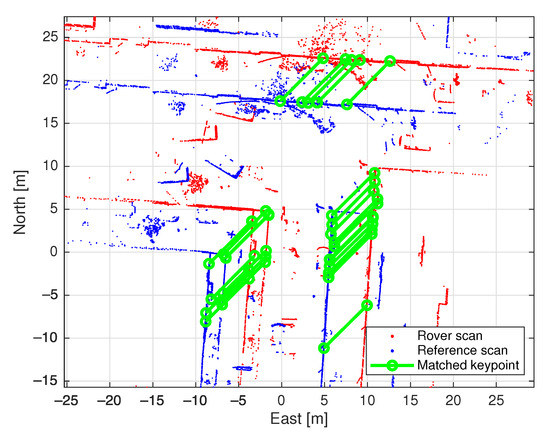
Figure 1.
Example of matched keypoints.
2.3. Estimating Vehicle Position
Provided that corresponding keypoints between the rover scan and the identified reference scan are successfully obtained through RANSAC, the position of the vehicle in e-frame can be computed as the translational component of the transformation from the rover scan (in b-frame) to the reference scan, since the origins of the point clouds are equivalent to the vehicle position. For a corresponding pair of keypoints in the rover scan, the following transformation can be constructed:
where the vector denotes the coordinates of in e-frame from the reference scan, while the measured vector denotes the coordinates of in b-frame from the rover scan. The corresponding measurement residual vector is denoted by . The rotational parameters are given by (), with being the vector of translational parameters, thus the vehicle position in e-frame. Here and in the following, the superscript indicates the ‘transpose’ of a vector/matrix. Vectors and matrices are distinguished from scalars by bold-italic lowercase and uppercase letters, respectively. Thus x is a scalar, is a vector, and is a matrix. The vehicle position can be resolved by, for instance, a Weighted Least-Squares (WLS) method with at least four matched keypoints. The weights of measurements, denoted by , can be determined using the mean-squared residual distance between the corresponding keypoints matched through RANSAC as follows
with the mean-squared residual distance , where is the residual distance between the transformed and its matched keypoint from the reference scan. is the identity matrix of order 3. The total number of corresponded keypoints is denoted by n.
3. EKF Formulation via a Mixed Measurement Model
The lidar positioning solutions can be absent when there is a lack of matched keypoints. This can happen when the HD map is not up-to-date as it is collected from a previous time and does not reflect changes in the road environments captured in the rover scans. To avoid such a lack of solution, we propose to combine lidar measurements with GNSS code measurements at the observation level. This integrated approach aims to take advantage of the two complimentary sensors, so that when the numbers of measurements from either or both sensors are insufficient for standalone positioning, they could still enable the integration. In this section, we discuss our strategy for combining the lidar and GNSS code measurements so as to deliver seamless positioning solutions. Both single- and multi-epoch positioning solutions are considered. The term ‘single-epoch’ refers to the solutions for which use is made of only one epoch of measurements, whereas the term ‘multi-epoch’ refers to the solutions for which an EKF formulation is employed to incorporate the time-behavior of the vehicle motion into the model, thus benefiting from the measurements of previous epochs.
3.1. Lidar and GNSS Observation Equations
To set up our EKF formulation, we first commence with the observation equations on which the positioning solution is based. With reference to (1), the lidar observation equations of keypoint take the following vectorial form:
in which the unknown vectors and are to be estimated through the measurement vectors and the known coordinates (). is a vector of zeros. The symbol ⊗ denotes the matrix Kronecker product [25]. Next to the above lidar observation equations, the observation equation of the single-frequency GNSS SPP model reads [26]:
where denotes the GNSS code measurement of satellite s that has already been corrected for the effect of satellite clock offsets. The ionospheric and tropospheric delays are also partially removed from the code measurement using atmospheric corrections from Klobuchar and Saastamoinen models, respectively [27]. The code measurement residuals are denoted by . The known position vector of satellite s is denoted by that is available in GNSS broadcast orbit files. Next to the vehicle position , the unknown receiver clock offset (expressed in meters rather than in seconds) is to be estimated through the measurements (), where m is the number of visible GNSS satellites. Note that the coordinates used in (4) are in e-frame. As with the lidar measurement weights (2), an appropriate choice of weights is required to weight the GNSS code measurements. These weights, denoted by , can be given by
where denotes the GNSS User Equivalent Range Error (UERE) which varies between 0.5 and 6 m. Accordingly, the weights are increasing functions of the satellite elevation . The larger the satellite elevation, the more precise the GNSS measurement is assumed, thus the higher the weight of the measurement becomes.
3.2. Filter Setup
The comparison of the system of lidar observation Equation (3) with its GNSS version (4) shows that both have the unknown vehicle position vector in common. One can therefore combine these two systems of equations so as to obtain a solution for in an optimal manner. We use the least-squares principle as the optimality criterion [28]. Accordingly, the two systems of Equations (3) and (4) can be expressed in a more compact form as follows:
where the unknown parameter vector contains the vehicle position vector (i.e., the lidar translational parameters), the GNSS receiver clock offset , and the lidar rotational parameters . Thus, . The measurement vector contains the lidar measurements () and GNSS code measurements (), with being the corresponding residual vector which contains () and (). The entries of the vector function are formed by the observation Equations (3) and (4). The linearized form, on the right-hand side of (6), follows as the first-order Taylor expansion of about the point , where indicates the approximate version of the parameter vector , leading to the unknown increment vector . Thus, . The known matrices and are the Jacobian matrices of with respect to and , respectively. Their explicit structures are presented in Appendix A. Defining the block diagonal matrix operator as , which aligns input matrices along the diagonal of a square matrix, the weight matrix is constructed as (i.e., is identical to the inverse of the measurements’ variance matrix). Hence, an application of the WLS principle to (6) gives [28]:
with . This gives the WLS solution for the unknown parameter vector as . The above procedure is iteratively repeated by replacing the solution with the approximate vector until the solution convergence is declared by, for example, having the magnitude of the increment vector smaller than a threshold. Matrix would represent the error-variance matrix of the solution if the weight matrix is the inverse of the measurements’ variance matrix. The solution can be regarded as the ‘single-epoch’ solution as it does not use any information about the time-behavior of the vehicle motion. This solution can be used to initialize the EKF.
3.3. Filter Time-Update
Let us now assume that the acceleration of the vehicle motion can be modeled by a zero-mean white-noise vector with three distinct spectral densities in ENU-directions. In other words, the vehicle motion is assumed to obey a ‘constant-velocity’ model on average. Now let be the solution of the vehicle position at epoch . According to the constant-velocity model, the position of the vehicle and its velocity at the forthcoming epoch k can be predicted (or time-updated) as [29]:
where and denote the solutions of the vehicle position and velocity vectors at epoch k, respectively. The measurement sampling rate is given by . Given the error-variance matrix of the previous solution , say , the error-variance matrix of the time-updated solution can be computed as [29]:
in which the transition matrix and matrix are given by:
The rotation matrix makes the ENU-direction parallel to the e-frame. The diagonal matrix is formed by the ENU spectral densities of the vehicle acceleration vector. The stated spectral densities are (for East), (for North) and (for Up). In this study, the spectral densities are specified as and .
3.4. Filter Measurement-Update
In the event that no lidar nor GNSS measurements are available, the time-update solution can serve as a solution for the vehicle position and velocity. In the presence of measurements, however, the time-update Equation (8) can be augmented with our earlier system of observation, Equation (6), to deliver the so-called measurement-update solution [29]. Since this solution benefits from the information of the time-update (8), and therefore that of the previous epochs, we also refer to this solution as the ‘multi-epoch’ solution. Thus the measurement-update of our EKF formulation can be computed in an analogous way to that of the WLS solution (7), with a difference, in that the system of observations (6) is replaced by:
The structure of the vector function , together with those of , , and , is given in Appendix A. Therefore, in order to obtain the measurement-update solution for , one should replace by , by , by ‘’, and by . Likewise, the weight matrix should be replaced by ‘’. In the next section, the numerical performance of our proposed EKF formulation is assessed under several scenarios.
4. Experimental Setup and Results
In Section 2 and Section 3, we provided the lidar positioning model and the EKF formulation. In this section we present experiments of three positioning methods derived accordingly, including two single-epoch methods: (1) GNSS SPP uses single-frequency GNSS code measurements from the Beidou constellation; and (2) Lidar-only uses only lidar registration as described in Section 2. They are then combined at the observation level and extended to a multi-epoch positioning method by enabling the constant-velocity time-update in EKF as explained in Section 3; namely (3) Integrated.
In order to evaluate the performance of the proposed positioning approaches, we make the following definitions:
- Lidar keypoint matching success rate is defined as the proportion of the epochs with successfully identified corresponding keypoints which contribute to lidar measurements;
- Availability is defined as the proportion of the epochs with positioning solutions under a specified error threshold;
- Accuracy is measured by the Root Mean Squared Error (RMSE) of the offsets of the positioning solutions from the ground truth.
4.1. Experimental Setup
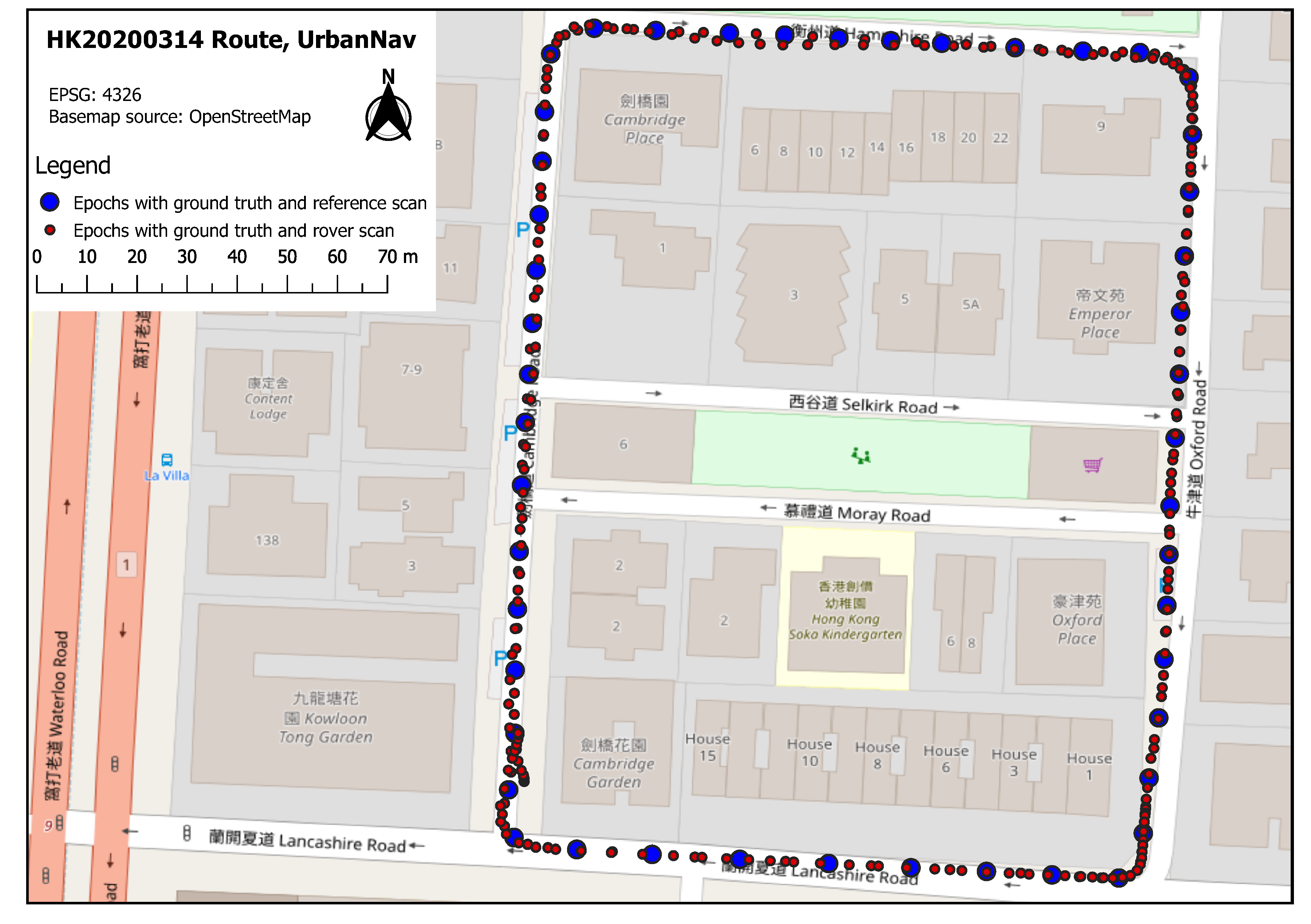
The proposed methods are evaluated on a Hong Kong drive from the UrbanNav [30] dataset as shown in Figure 2, which is captured in a densely built-up urban environment, where GNSS is deprived. The vehicle used for data collection is equipped with the following sensors:
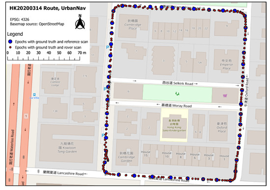
Figure 2.
HK20200314 route in UrbanNav [30].
- Velodyne HDL-32E lidar sensor;
- Xsens Mti 10 IMU;
- U-blox M8T GNSS receiver;
- RGB Camera;
- SPAN-CPT GNSS-RTK/INS integrated system.
The SPAN-CPT system provides the ground truth data including accurate 3D coordinates of the vehicle and relative roll, pitch and yaw angles, which operates at 1 Hz, as well as the low-cost U-blox M8T receiver that collects Beidou single-frequency observations. The lidar sensor operates at 10 Hz, and the collected point clouds are synchronized with the GNSS sensors for the experiments. Each captured point cloud contains approximately 65,000 3D points and occupies 5 MB of storage [30]. The remaining two sensors, namely the IMU and camera, are not used in the experiments since they are not required by the proposed method.
In order to obtain the georeferencing transformation matrix for a reference scan, each point in the scan is transformed from l-frame to b-frame, then to e-frame. For the ith () point cloud in a sequence, the first transformation matrix is pre-calibrated and provided in the dataset. All the point clouds in the sequence are first transformed to the b-frame of the first one using the roll, pitch, yaw angles and the differences between their ground truth coordinates, producing . As a result, with the coordinates of the origin for each scan in both e-frame and b-frame of the first point cloud, for the whole sequence can be estimated in a similar way as depicted in Section 2.3. As a short form, the three transformations can be combined as:
In total, ground truth data are recorded for 300 epochs. By specifying at least 10 m between every two consecutive reference scans, 47 point clouds are used as reference scans (HD map), the remaining 253 point clouds are used as rover scans for positioning. Note that the vehicle makes two laps along the trajectory shown in Figure 2.
4.2. Positioning Results under Ideal Lidar Conditions
In order to test the transferability of MS-SVConv [22], the model pre-trained with ETH dataset [31] is used. In the inference stage, is chosen as 5 to identify the reference scan for each rover scan. While estimating the transformation to align the two point clouds with RANSAC, 3000 random keypoints and their feature vectors are used after ground removal. As a result, all rover scans are successfully matched with the HD map and the mean RMSE of residual distances of the corresponding keypoints matched with RANSAC is approximately 0.07 m. This shows that reference scans can be found for 100% of the rover scans under ideal circumstances (i.e., lidar keypoint matching success rate is 100%), which we consider an acceptable transferability for our experiment. Note that this high keypoint matching success rate is made possible by the fact that the reference and rover scans are from the same dataset, which was collected within minutes, meaning that the temporal changes of the road environment are minimal.
To demonstrate the availability and accuracy of the three positioning methods, we compute the position estimation errors with respect to the ground truth. Table 1 presents the 2D, or horizontal RMSE and 3D RMSE of all tested methods. We first draw attention to the more accurate Lidar-only and Integrated results, whose 3D RMSE are 1.716 m and 1.445 m respectively for the 253 epochs with successfully matched keypoints, achieving accuracy within 2 m. This shows that when lidar keypoint matching success rate is 100% under ideal lidar conditions, positioning with only lidar input can already provide accurate solutions, and the integration with the less accurate GNSS code measurements offers little improvement.

Table 1.
Two-dimensional (2D), 3D RMSE and minimum, maximum 3D errors of the solutions from GNSS SPP, Lidar-only and Integrated positioning methods with 100% lidar keypoint matching success rate.
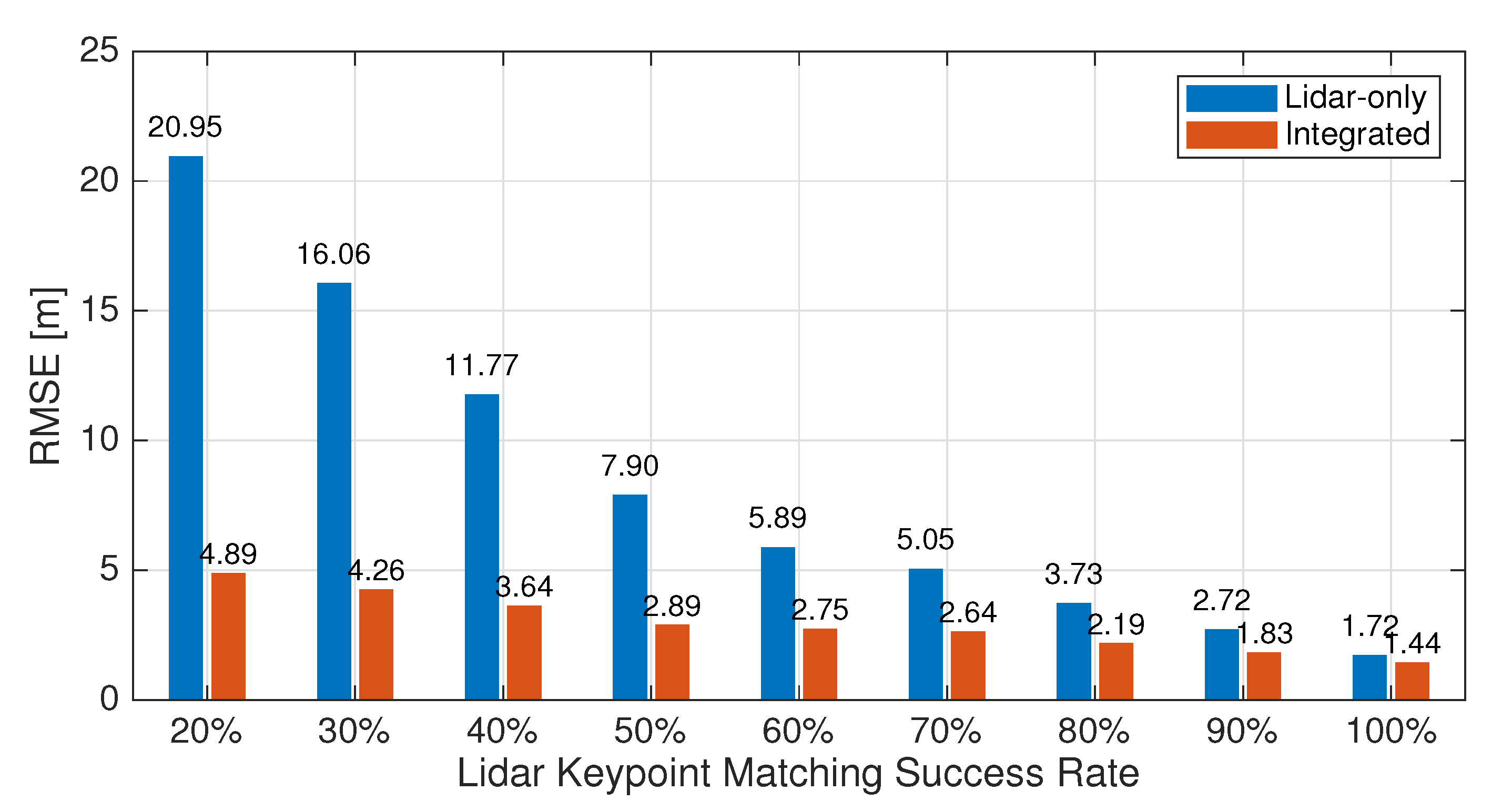
However, we recognize that the 100% lidar keypoint matching success rate is optimistic and unrealistic. In reality, with the HD map consisting of reference scans collected from a previous time, the environmental changes and moving objects such as pedestrians and vehicles can cause disturbance for point cloud registration and lead to failure of keypoint matching. Since RANSAC picks random points and their feature vectors to find correspondence such as static objects, it can handle differences between two point clouds to a certain extent [32]. Therefore, to emphasize the accuracy improvement brought by the proposed integration, we have simulated different lidar keypoint matching success rates between 20% and 90% by disabling lidar measurements for randomly selected epochs to compare Lidar-only and Integrated. For any epoch that fails keypoint matching, the positioning solution from the last-available epoch is used. Figure 3 shows the 3D RMSE of the positioning errors using these two methods. As previously discussed, the accuracy of Integrated is only 0.271 m better than Lidar-only at 100%. However, as the lidar keypoint matching success rate decreases, the margin between the two increases dramatically, with Integrated having consistently higher accuracy than Lidar-only. In the worst case scenario where only 20% of the epochs have lidar contribution, the 3D RMSE of Lidar-only reaches 20.95 m whereas Integrated can still keep it below 10 m at 4.89 m. In the remainder of this section, we will set the lidar keypoint matching success rate as 80% to present the positioning performance of the proposed method in practical urban environments.

Figure 3.
RMSE of 3D errors of Lidar-only and Integrated solutions at various simulated lidar keypoint matching success rates.
4.3. Positioning Results in Realistic Environments
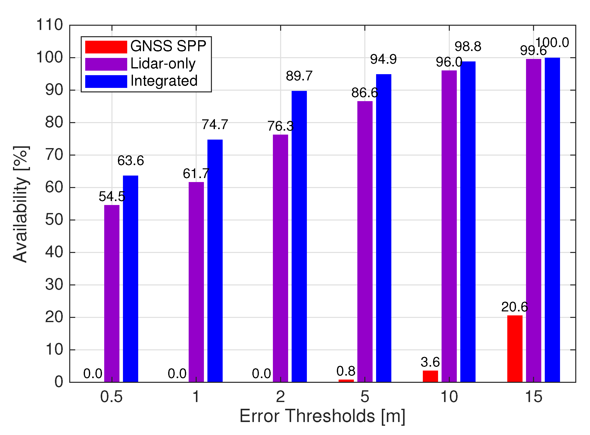
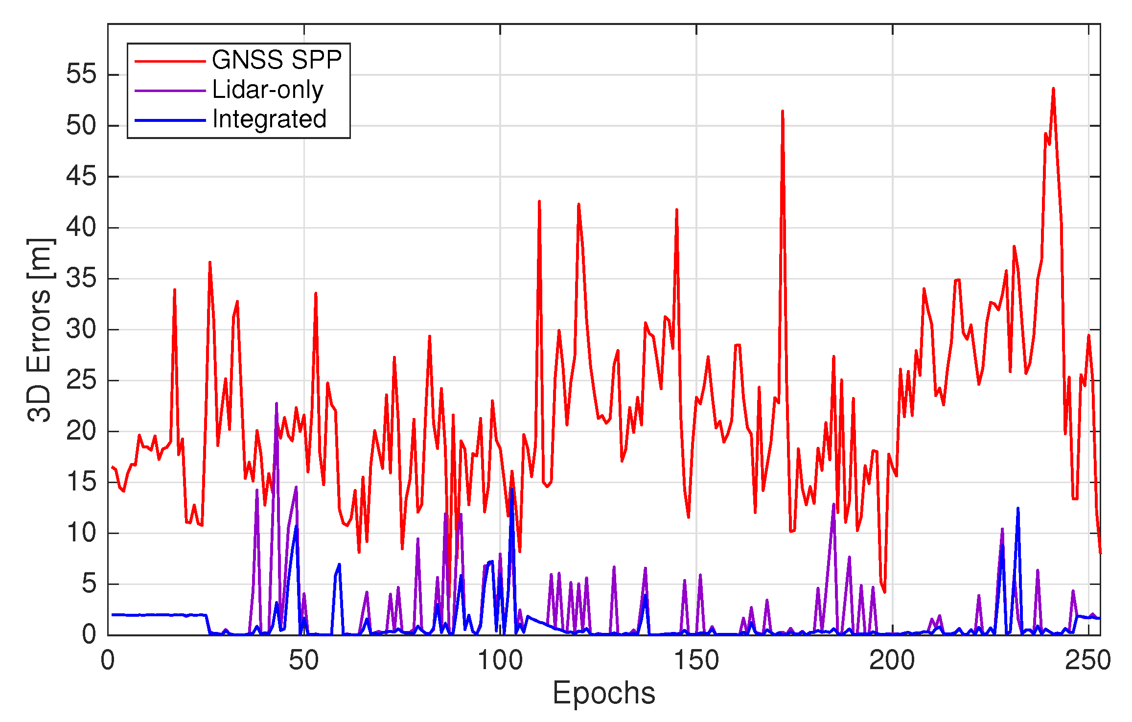
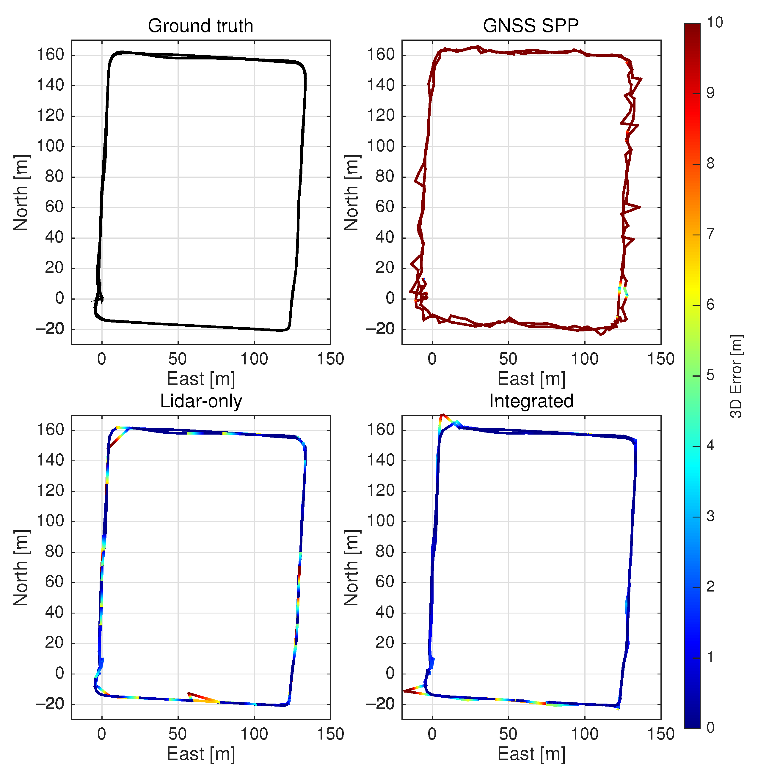
We now evaluate the three positioning methods on practical urban roads by simulating the lidar keypoint matching success rate as 80%. The RMSE, minimum and maximum errors of the positioning solutions are presented in Table 2. For the Lidar-only method, the 2D and 3D RMSE of the positioning solutions are 5.024 m and 5.050 m, respectively. Figure 4 compares all tested positioning methods in terms of the availabilities of solutions under different 3D error thresholds. The error thresholds are chosen between 0.5 m, which has been suggested as the required accuracy for lane-level positioning [2], and 15 m which is approximately the largest error of the Integrated positioning solutions (see Table 2). It is shown that for Lidar-only, 76.3% of the solutions have 3D errors smaller than or equal to 2 m, while the minimum is 0.019 m and the maximum is 22.748 m, as illustrated in Figure 5 that shows the 3D errors per epoch. Figure 6 presents the horizontal trajectories of solutions from all tested methods comparing with the ground truth. It is evident that Lidar-only solutions correspond with the ground truth well, except for epochs missing lidar measurements that are left with the last-available solutions.

Table 2.
Two-dimensional (2D), 3D RMSE and minimum, maximum 3D errors of the solutions from GNSS SPP, Lidar-only and Integrated positioning methods with 80% lidar keypoint matching success rate.
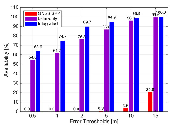
Figure 4.
Availabilities of solutions under different 3D error thresholds for GNSS SPP, Lidar-only and Integrated positioning methods.

Figure 5.
3D offsets from ground truth for GNSS SPP, Lidar-only and Integrated solutions.
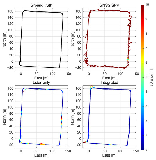
Figure 6.
The 2D trajectories of solutions from GNSS SPP, Lidar-only and Integrated positioning methods [33].
In comparison, by specifying the elevation cutoff angle of 10°, GNSS SPP solutions are computed. Consequently, the 2D and 3D RMSE from given ground truth are 4.888 m and 23.197 m, respectively, while solutions are obtained for all epochs thanks to the abundant Beidou satellites (Table 2). However, Figure 4 suggests that the availability of GNSS SPP solutions is significantly lower than those of Lidar-only at all error thresholds and the maximum 3D error is 53.685 m (Figure 5). Moreover, Figure 6 shows that the GNSS SPP positioning results consistently contain the largest errors for the whole trajectory.
We now show the availability and accuracy of the integrated multi-epoch positioning approach using the same data. By using the constant-velocity time-update in the EKF, positioning solutions are obtained for 100% of the tested epochs for the Integrated method. The 2D and 3D RMSE of its solutions can be found in Table 2. Notably, the accuracy of Integrated is the highest among all three, with the 3D RMSE being 2.187 m, and the minimum and maximum 3D errors being 0.019 m and 14.359 m (Figure 5). In terms of availability, Figure 4 suggests that all epochs are with errors smaller than or equal to 15 m for Integrated, while it outperforms the other two methods at every error threshold. Lastly, Figure 6 presents that the trajectories of Lidar-only and Integrated results have similar and the higher agreement with the ground truth, yet Integrated has fewer epochs with large errors.
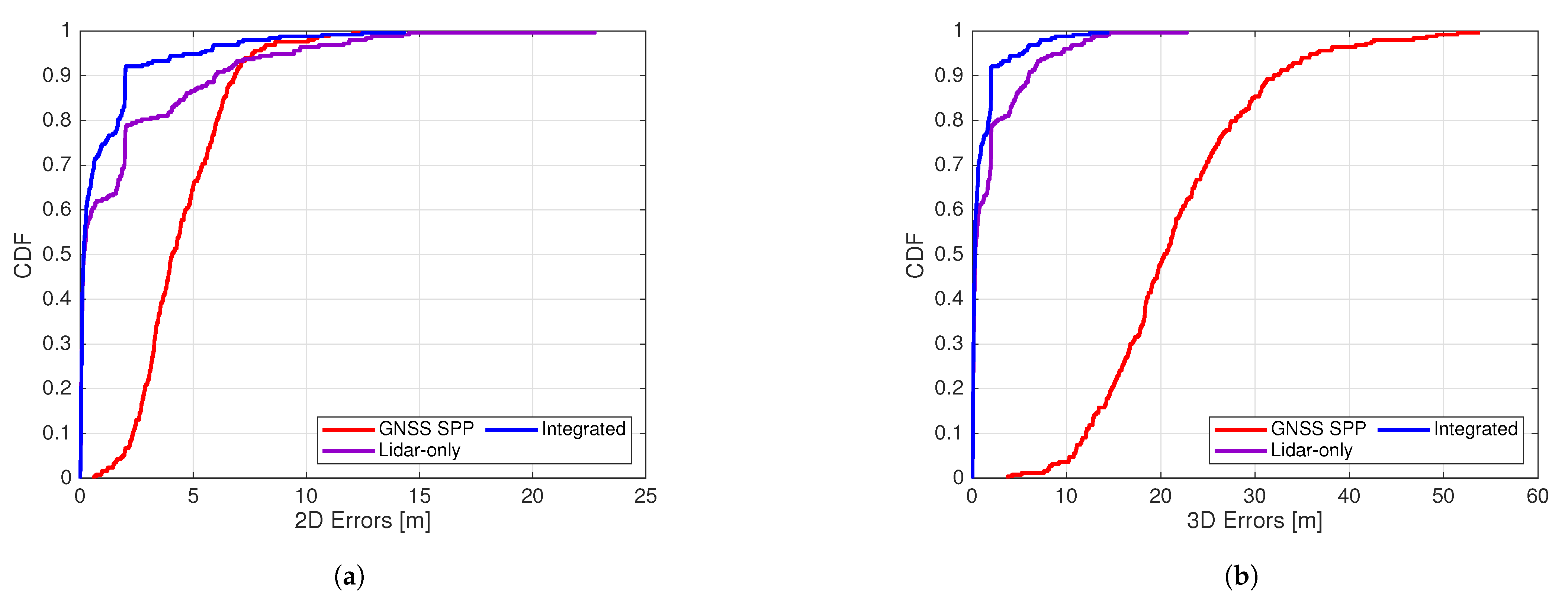
Figure 7 illustrates the cumulative distributions of 2D (horizontal) and 3D errors for all methods. It can be seen that the positioning methods involving lidar measurements, namely Lidar-only and Integrated, both outperform GNSS SPP, which only takes the less accurate GNSS code observations as measurements, especially in the vertical component. Integrated is clearly the most accurate among all three.
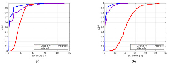
Figure 7.
Cumulative distributions of 2D and 3D offsets from ground truth for all methods. (a) Cumulative distributions of 2D offsets from ground truth for all methods. (b) Cumulative distributions of 3D offsets from ground truth for all methods.
5. Discussion
5.1. Significant GNSS Code Errors
It is evident from Figure 4 and Table 2 that the errors of the GNSS SPP method are considerably larger than the others, especially in the Up component. Apart from the low precision of the GNSS code measurements and the use of only single-frequency data, an important reason for this behavior is the significant multipath effect. The tested drive took place in Hong Kong, which is a city with dense buildings. Wen et al. [4] performed experiments with a similar setup and concluded that approximately 2 to 7 satellites can be blocked or reflected to produce non-line-of-sight signals for each epoch. This implies that solely SPP with code measurements is inappropriate for vehicle positioning in urban canyons. To this end, our results have shown that the addition of lidar registration can greatly improve the accuracy.
5.2. Keypoint Matching Errors and Failure
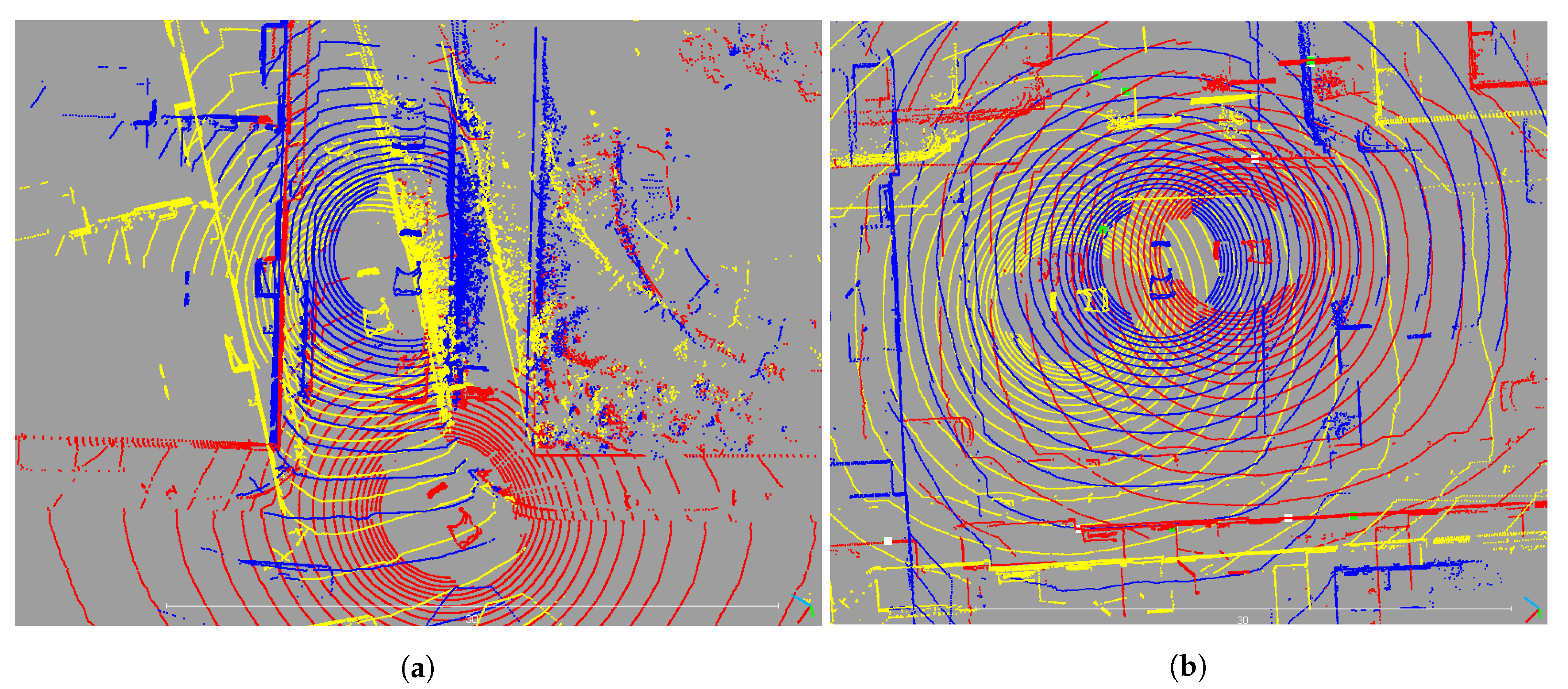
Although the Lidar-only approach achieves a much higher accuracy than GNSS SPP when lidar measurements are available, it can still be degraded by different error sources. First of all, since the lidar positioning approach is relative to the reference scans, the performance is greatly affected by the quality of the HD map. For example, Figure 8a presents a scenario in which the reference scan is poorly georeferenced. As the position of the vehicle is obtained by registering the rover scan to the reference scan, the resolved vehicle position is meters away from the ground truth. This behavior is frequently observed around road intersections where the vehicle is turning and the inertial measurements contributing to the ground truth used for georeferencing become less reliable. Secondly, Figure 8b shows that keypoint matching can also be impacted by the surrounding environment. Wrong registration might occur when the point clouds contain noise such as vegetation and moving objects, or when there are environmental changes due to the reference scans being collected from a previous time, which leads to falsely matched keypoints whose feature vectors are similar by coincidence.
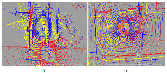
Figure 8.
Examples of lidar error sources. Red: reference scan from the HD map. Yellow: ground truth point cloud of the rover scan. Blue: Rover scan registered by MS-SVConv. (a) Example of lidar errors produced by anomalies in the HD map. (b) Example of lidar errors produced by false matching.
5.3. Accuracy and Availability Improvements Brought by the Integration
It can be seen from Figure 5 and Figure 6 that the results of the Integrated method are nearly identical to those of Lidar-only when lidar measurements exist. This is due to the high accuracy of the lidar measurements produced from deep-learning point cloud registration. In other words, the Integrated method is similar to the Lidar-only method if the latter can function well. In comparison, when lidar positioning fails due to the lack of matched keypoints, the Lidar-only method would use the positioning solutions from the last-available epochs, ignoring the movement of the vehicle. Therefore, in the case of having no lidar measurements, the positioning errors would be considerably larger. This motivated the utilization of constant-velocity time-update in EKF, which largely increased the accuracy of the integration.
To highlight the accuracy and availability improvements brought by the EKF, the magnitudes of the 3D errors over all epochs for the three single-epoch methods and Integrated are shown in Figure 5. It is apparent that Integrated consistently achieves the smallest errors among all, whereas the accuracy of GNSS SPP is significantly worse than the others. Although Lidar-only can obtain similar accuracy as Integrated for most of the duration, the addition of the EKF is able to decrease the larger errors caused by the absence of lidar measurements.
5.4. Keypoint Matching Success Rate Simulation and Comparison
Section 4.2 suggests that, under ideal circumstances, Lidar-only and Integrated can both obtain metre-level accuracy. However, when the lidar keypoint matching success rate is lower, which is more realistic for large-scale HD map products, the advantage of the integration becomes more noticeable, as shown in Figure 3. Therefore, although positioning by lidar registration has a high accuracy, it can be dramatically degraded by possible failure of keypoint matching, whereas the less accurate GNSS code can be complimentary due to the abundance of GNSS satellites and the modeling of the vehicle dynamics using the constant-velocity time-update to consistently retain metre-level accuracy. In contrast, the accuracy of lidar positioning quickly deteriorates. In other words, the addition of GNSS code measurements and EKF to the lidar registration positioning can greatly decrease the positioning errors when the lidar keypoint matching success rate is low.
5.5. Runtime Efficiency
The implementation of the proposed integrated positioning method is divided into two stages: keypoint matching stage and positioning stage, with the former employing the PyTorch [34] implementation of MS-SVConv [22] and the latter computing the measurements and positioning solutions in MATLAB [35]. On a platform consisting of AMD Ryzen 3800XT CPU (4.4 GHz) and NVIDIA RTX 3070 GPU, the keypoint matching stage and the positioning stage consume approximately 0.85 s and 0.05 s, respectively, per epoch. Therefore, the proposed approach is capable of real-time positioning.
6. Conclusions
In this paper, we proposed an integration of lidar and GNSS code measurements at the observation level in a constant-velocity Extended Kalman-Filter. A deep learning mechanism named MS-SVConv was used to match rover scans with reference scans from a pre-built HD map that contains georeferenced point clouds of segments of the road environments. Lidar measurements were generated from the corresponding keypoints between the two point clouds, and combined with single-frequency GNSS code measurements via a mixed measurement model. To capture the dynamics of the vehicle movement, we made use of a constant velocity model in ENU directions with distinct spectral densities for the corresponding vehicle acceleration vector.
Experimental results showed that the proposed method can achieve centimeter- to meter-level accuracy for vehicle positioning in urban canyons for the entire duration, and can also greatly increase the availability of low-error positioning solutions compared with standalone methods, as the RMSE, minimum and maximum values of the 3D errors were 2.187 m, 0.019 m and 14.359 m, respectively at an 80% lidar keypoint matching success rate. The main contributions of this study are summarized as follows:
- Lidar measurements are generated using a deep learning mechanism through point cloud registration with a pre-built HD map for positioning purposes;
- It was demonstrated that the proposed positioning approach (Integrated) can achieve centimeter- to meter-level 3D accuracy for the entirety of the driving duration in densely built-up urban environments, where the accuracy of GNSS code measurements is low and standalone lidar positioning may not always be available;
- When the keypoint matching success rate is low, as can be expected for a realistic scenario, the proposed Integrated approach provides the best accuracy while maintaining 100% availability of positioning solutions.
While the proposed method achieves meter- to submeter-level seamless positioning by exploiting the complimentary properties of GNSS code and lidar measurements, future research can explore increasing the accuracy by extending the integration using other types of measurements such as GNSS carrier phase observations and inertial measurements from IMU.
Author Contributions
Conceptualization, J.Z., K.K. and A.K.; methodology, J.Z., K.K. and A.K.; software, J.Z. and A.K.; validation, J.Z., K.K. and A.K.; formal analysis, J.Z.; investigation, J.Z., K.K. and A.K.; resources, J.Z.; data curation, J.Z.; writing—original draft preparation, J.Z.; writing—review and editing, K.K. and A.K.; visualization, J.Z. and K.K.; supervision, K.K. and A.K.; project administration, K.K. and A.K. All authors have read and agreed to the published version of the manuscript.
Funding
This research received no external funding.
Data Availability Statement
Not applicable.
Acknowledgments
This research did not receive any specific grant from funding agencies in the public, commercial, or not-for-profit sectors. The first author acknowledges the financial support from The University of Melbourne through the Melbourne Research Scholarship.
Conflicts of Interest
The authors declare no conflict of interest.
Abbreviations
The following abbreviations are used in this manuscript:
| EKF | Extended Kalman-Filter |
| GNSS | Global Navigation Satellite System |
| GPS | Global Positioning System |
| HD | High definition |
| ICP | Iterative Closest Point |
| IMU | Inertial Measurement Unit |
| Lidar | Light detection and ranging |
| RANSAC | Random Sample Consensus |
| RMSE | Root Mean Squared Error |
| RTK | Real-time Kinematic |
| SLAM | Simultaneous Localization and Mapping |
| SPP | Standard Point Positioning |
| UERE | User Equivalent Range Error |
| WLS | Weighted Least-Squares |
Appendix A. Jacobian Matrices of the Mixed Models (6) and (11)
The structures of the Jacobian matrices and , in the mixed model (6), are given by
in which the rows of the sub-matrix are the satellite-to-receiver direction (unit) vectors (). The matrices of zeros and ones are, respectively, denoted by and , where their dimension is specified by a subscript. The sub-matrix and the rotation matrix read
As for the ‘multi-epoch’ version (11), the time-updated solution plays the role of extra measurements, while the parameter vector is augmented with the vehicle velocity vector , that is, . Thus matrix , in (A1), is extended as . Likewise, the corresponding vector function reads
from which the Jacobian matrices and follow as
Finally, the vector is evaluated as .
References
- Rödel, C.; Stadler, S.; Meschtscherjakov, A.; Tscheligi, M. Towards autonomous cars: The effect of autonomy levels on acceptance and user experience. In Proceedings of the 6th International Conference on Automotive User Interfaces and Interactive Vehicular Applications, Seattle, DC, USA, 17–19 September 2014; pp. 1–8. [Google Scholar]
- Joubert, N.; Reid, T.G.; Noble, F. Developments in modern GNSS and its impact on autonomous vehicle architectures. In Proceedings of the 2020 IEEE Intelligent Vehicles Symposium (IV), Las Vegas, NV, USA, 19 October–13 November 2020; pp. 2029–2036. [Google Scholar]
- Hofmann-Wellenhof, B.; Lichtenegger, H.; Wasle, E. GNSS: Global Navigation Satellite Systems: GPS, Glonass, Galileo, and More; Springer: New York, NY, USA, 2008. [Google Scholar]
- Wen, W.; Zhang, G.; Hsu, L.T. Correcting NLOS by 3D LiDAR and building height to improve GNSS single point positioning. Navigation 2019, 66, 705–718. [Google Scholar] [CrossRef]
- Ghallabi, F.; Nashashibi, F.; El-Haj-Shhade, G.; Mittet, M.A. LIDAR-based lane marking detection for vehicle positioning in an HD map. In Proceedings of the 2018 21st International Conference on Intelligent Transportation Systems (ITSC), Maui, HI, USA, 4–7 November 2018; pp. 2209–2214. [Google Scholar]
- Ramezani, M.; Khoshelham, K. Vehicle positioning in GNSS-deprived urban areas by stereo visual-inertial odometry. IEEE Trans. Intell. Veh. 2018, 3, 208–217. [Google Scholar] [CrossRef]
- Nadarajah, N.; Khodabandeh, A.; Wang, K.; Choudhury, M.; Teunissen, P.J.G. Multi-GNSS PPP-RTK: From large-to small-scale networks. Sensors 2018, 18, 1078. [Google Scholar] [CrossRef] [PubMed] [Green Version]
- Khodabandeh, A.; Zaminpardaz, S.; Nadarajah, N. A study on multi-GNSS phase-only positioning. Meas. Sci. Technol. 2021, 32, 095005. [Google Scholar] [CrossRef]
- Teunissen, P.J.G.; de Jonge, P.J.; Tiberius, C.C.J.M. The least-squares ambiguity decorrelation adjustment: Its performance on short GPS baselines and short observation spans. J. Geod. 1997, 71, 589–602. [Google Scholar] [CrossRef] [Green Version]
- Humphreys, T.E.; Murrian, M.J.; Narula, L. Deep-Urban Unaided Precise Global Navigation Satellite System Vehicle Positioning. IEEE Intell. Transp. Syst. Mag. 2020, 12, 109–122. [Google Scholar] [CrossRef]
- Braasch, M.S. Multipath. In Springer Handbook of Global Navigation Satellite Systems; Springer: Berlin/Heidelberg, Germany, 2017; pp. 443–468. [Google Scholar]
- Maaref, M.; Khalife, J.; Kassas, Z.M. Lane-level localization and mapping in GNSS-challenged environments by fusing lidar data and cellular pseudoranges. IEEE Trans. Intell. Veh. 2018, 4, 73–89. [Google Scholar] [CrossRef]
- Liu, R.; Wang, J.; Zhang, B. High definition map for automated driving: Overview and analysis. J. Navig. 2020, 73, 324–341. [Google Scholar] [CrossRef]
- Wang, L.; Zhang, Y.; Wang, J. Map-based localization method for autonomous vehicles using 3D-LIDAR. IFAC-PapersOnLine 2017, 50, 276–281. [Google Scholar] [CrossRef]
- Im, J.H.; Im, S.H.; Jee, G.I. Extended line map-based precise vehicle localization using 3D LIDAR. Sensors 2018, 18, 3179. [Google Scholar] [CrossRef] [PubMed] [Green Version]
- Ghallabi, F.; El-Haj-Shhade, G.; Mittet, M.A.; Nashashibi, F. LIDAR-Based road signs detection For Vehicle Localization in an HD Map. In Proceedings of the 2019 IEEE Intelligent Vehicles Symposium (IV), Paris, France, 9–12 June 2019; pp. 1484–1490. [Google Scholar]
- Rusinkiewicz, S.; Levoy, M. Efficient variants of the ICP algorithm. In Proceedings of the Third International Conference on 3-D Digital Imaging and Modeling, Quebec City, QC, Canada, 28 May–1 June 2001; pp. 145–152. [Google Scholar] [CrossRef] [Green Version]
- Zhang, Z.; Dai, Y.; Sun, J. Deep learning based point cloud registration: An overview. Virtual Real. Intell. Hardw. 2020, 2, 222–246. [Google Scholar] [CrossRef]
- Mueller, K.; Atman, J.; Kronenwett, N.; Trommer, G.F. A Multi-Sensor Navigation System for Outdoor and Indoor Environments. In Proceedings of the 2020 International Technical Meeting of The Institute of Navigation, San Diego, CA, USA, 21–24 January 2020; pp. 612–625. [Google Scholar]
- Li, N.; Guan, L.; Gao, Y.; Du, S.; Wu, M.; Guang, X.; Cong, X. Indoor and Outdoor Low-Cost Seamless Integrated Navigation System Based on the Integration of INS/GNSS/LIDAR System. Remote Sens. 2020, 12, 3271. [Google Scholar] [CrossRef]
- Qian, C.; Zhang, H.; Li, W.; Shu, B.; Tang, J.; Li, B.; Chen, Z.; Liu, H. A LiDAR aiding ambiguity resolution method using fuzzy one-to-many feature matching. J. Geod. 2020, 94, 98. [Google Scholar] [CrossRef]
- Horache, S.; Deschaud, J.E.; Goulette, F. 3D Point Cloud Registration with Multi-Scale Architecture and Self-supervised Fine-tuning. arXiv 2021, arXiv:2103.14533. [Google Scholar]
- Fischler, M.A.; Bolles, R.C. Random sample consensus: A paradigm for model fitting with applications to image analysis and automated cartography. Commun. ACM 1981, 24, 381–395. [Google Scholar] [CrossRef]
- Himmelsbach, M.; Hundelshausen, F.V.; Wuensche, H.J. Fast segmentation of 3D point clouds for ground vehicles. In Proceedings of the 2010 IEEE Intelligent Vehicles Symposium, La Jolla, CA, USA, 21–24 June 2010; pp. 560–565. [Google Scholar]
- Henderson, H.V.; Pukelsheim, F.; Searle, S.R. On the History of the Kronecker Product. Linear Multilinear Algebra 1983, 14, 113–120. [Google Scholar] [CrossRef] [Green Version]
- Langley, R.B.; Teunissen, P.J.; Montenbruck, O. Introduction to GNSS. In Springer Handbook of Global Navigation Satellite Systems; Springer: Berlin/Heidelberg, Germany, 2017; pp. 3–23. [Google Scholar]
- Hobiger, T.; Jakowski, N. Atmospheric signal propagation. In Springer Handbook of Global Navigation Satellite Systems; Springer: Berlin/Heidelberg, Germany, 2017; pp. 165–193. [Google Scholar]
- Teunissen, P.J.G. Adjustment Theory: An Introduction; Series on Mathematical Geodesy and Positioning; Delft University Press: Delft, The Netherlands, 2000. [Google Scholar]
- Teunissen, P. Dynamic Data Processing; Recursive Least Squares; VSSD: Delft, The Netherlands, 2001. [Google Scholar]
- Wen, W.; Bai, X.; Hsu, L.T.; Pfeifer, T. GNSS/LiDAR Integration Aided by Self-adaptive Gaussian Mixture Models in Urban Scenarios: An Approach Robust to Non-Gaussian Noise. In Proceedings of the 2020 IEEE/ION Position, Location and Navigation Symposium (PLANS), Portland, OR, USA, 20–23 April 2020; pp. 647–654. [Google Scholar]
- Pomerleau, F.; Liu, M.; Colas, F.; Siegwart, R. Challenging data sets for point cloud registration algorithms. Int. J. Robot. Res. 2012, 31, 1705–1711. [Google Scholar] [CrossRef] [Green Version]
- Zhou, Q.Y.; Park, J.; Koltun, V. Open3D: A modern library for 3D data processing. arXiv 2018, arXiv:1801.09847. [Google Scholar]
- Grinsted, A. Subaxis-Subplot. 2021. Available online: https://au.mathworks.com/matlabcentral/fileexchange/3696-subaxis-subplot (accessed on 1 March 2021).
- Paszke, A.; Gross, S.; Massa, F.; Lerer, A.; Bradbury, J.; Chanan, G.; Killeen, T.; Lin, Z.; Gimelshein, N.; Antiga, L.; et al. PyTorch: An Imperative Style, High-Performance Deep Learning Library. In Advances in Neural Information Processing Systems 32; Wallach, H., Larochelle, H., Beygelzimer, A., d’Alché-Buc, F., Fox, E., Garnett, R., Eds.; Curran Associates, Inc.: Nice, France, 2019; pp. 8024–8035. [Google Scholar]
- MATLAB. 9.10.0.1710957 (R2021a); The MathWorks Inc.: Natick, MA, USA, 2021. [Google Scholar]
Publisher’s Note: MDPI stays neutral with regard to jurisdictional claims in published maps and institutional affiliations. |
© 2021 by the authors. Licensee MDPI, Basel, Switzerland. This article is an open access article distributed under the terms and conditions of the Creative Commons Attribution (CC BY) license (https://creativecommons.org/licenses/by/4.0/).


